ℹ️ Skipped - page is already crawled
| Filter | Status | Condition | Details |
|---|---|---|---|
| HTTP status | PASS | download_http_code = 200 | HTTP 200 |
| Age cutoff | PASS | download_stamp > now() - 6 MONTH | 0.1 months ago |
| History drop | PASS | isNull(history_drop_reason) | No drop reason |
| Spam/ban | PASS | fh_dont_index != 1 AND ml_spam_score = 0 | ml_spam_score=0 |
| Canonical | PASS | meta_canonical IS NULL OR = '' OR = src_unparsed | Not set |
| Property | Value |
|---|---|
| URL | https://www.probabilitycourse.com/chapter7/7_1_2_central_limit_theorem.php |
| Last Crawled | 2026-04-18 01:24:02 (2 days ago) |
| First Indexed | 2018-07-01 17:11:54 (7 years ago) |
| HTTP Status Code | 200 |
| Meta Title | Central Limit Theorem |
| Meta Description | null |
| Meta Canonical | null |
| Boilerpipe Text | The
central limit theorem (CLT)
is one of the most important results in probability theory. It states that, under certain conditions, the sum of a large number of random variables is approximately normal. Here, we state a version of the CLT that applies to i.i.d. random variables. Suppose that
X
1
,
X
2
, ... ,
X
n
are i.i.d. random variables with expected values
E
X
i
=
μ
<
∞
and variance
V
a
r
(
X
i
)
=
σ
2
<
∞
. Then as we saw above, the sample mean
X
¯
=
X
1
+
X
2
+
.
.
.
+
X
n
n
has mean
E
X
¯
=
μ
and variance
V
a
r
(
X
¯
)
=
σ
2
n
. Thus, the normalized random variable
Z
n
=
X
¯
−
μ
σ
/
n
=
X
1
+
X
2
+
.
.
.
+
X
n
−
n
μ
n
σ
has mean
E
Z
n
=
0
and variance
V
a
r
(
Z
n
)
=
1
. The central limit theorem states that the CDF of
Z
n
converges to the standard normal CDF.
The Central Limit Theorem (CLT)
Let
X
1
,
X
2
,...,
X
n
be i.i.d. random variables with expected value
E
X
i
=
μ
<
∞
and variance
0
<
V
a
r
(
X
i
)
=
σ
2
<
∞
. Then, the random variable
Z
n
=
X
¯
−
μ
σ
/
n
=
X
1
+
X
2
+
.
.
.
+
X
n
−
n
μ
n
σ
converges in distribution to the standard normal random variable as
n
goes to infinity, that is
lim
n
→
∞
P
(
Z
n
≤
x
)
=
Φ
(
x
)
,
for all
x
∈
R
,
where
Φ
(
x
)
is the standard normal CDF.
An interesting thing about the CLT is that it does not matter what the distribution of the
X
i
's is. The
X
i
's can be discrete, continuous, or mixed random variables. To get a feeling for the CLT, let us look at some examples. Let's assume that
X
i
's are
B
e
r
n
o
u
l
l
i
(
p
)
. Then
E
X
i
=
p
,
V
a
r
(
X
i
)
=
p
(
1
−
p
)
. Also,
Y
n
=
X
1
+
X
2
+
.
.
.
+
X
n
has
B
i
n
o
m
i
a
l
(
n
,
p
)
distribution. Thus,
Z
n
=
Y
n
−
n
p
n
p
(
1
−
p
)
,
where
Y
n
∼
B
i
n
o
m
i
a
l
(
n
,
p
)
. Figure 7.1 shows the PMF of
Z
n
for different values of
n
. As you see, the shape of the PMF gets closer to a normal PDF curve as
n
increases. Here,
Z
n
is a discrete random variable, so mathematically speaking it has a PMF not a PDF. That is why the CLT states that the CDF (not the PDF) of
Z
n
converges to the standard normal CDF. Nevertheless, since PMF and PDF are conceptually similar, the figure is useful in visualizing the convergence to normal distribution.
Fig.7.1 -
Z
n
is the normalized sum of
n
independent
B
e
r
n
o
u
l
l
i
(
p
)
random variables. The shape of its PMF,
P
Z
n
(
z
)
, resembles the normal curve as
n
increases.
As another example, let's assume that
X
i
's are
U
n
i
f
o
r
m
(
0
,
1
)
. Then
E
X
i
=
1
2
,
V
a
r
(
X
i
)
=
1
12
. In this case,
Z
n
=
X
1
+
X
2
+
.
.
.
+
X
n
−
n
2
n
/
12
.
Figure 7.2 shows the PDF of
Z
n
for different values of
n
. As you see, the shape of the PDF gets closer to the normal PDF as
n
increases.
Fig. 7.2 -
Z
n
is the normalized sum of
n
independent
U
n
i
f
o
r
m
(
0
,
1
)
random variables. The shape of its PDF,
f
Z
n
(
z
)
, gets closer to the normal curve as
n
increases.
We could have directly looked at
Y
n
=
X
1
+
X
2
+
.
.
.
+
X
n
, so why do we normalize it first and say that the normalized version (
Z
n
) becomes approximately normal? This is because
E
Y
n
=
n
E
X
i
and
V
a
r
(
Y
n
)
=
n
σ
2
go to infinity as
n
goes to infinity. We normalize
Y
n
in order to have a finite mean and variance (
E
Z
n
=
0
,
V
a
r
(
Z
n
)
=
1
). Nevertheless, for any fixed
n
, the CDF of
Z
n
is obtained by scaling and shifting the CDF of
Y
n
. Thus, the two CDFs have similar shapes.
The importance of the central limit theorem stems from the fact that, in many real applications, a certain random variable of interest is a sum of a large number of independent random variables. In these situations, we are often able to use the CLT to justify using the normal distribution. Examples of such random variables are found in almost every discipline. Here are a few:
Laboratory measurement errors are usually modeled by normal random variables.
In communication and signal processing, Gaussian noise is the most frequently used model for noise.
In finance, the percentage changes in the prices of some assets are sometimes modeled by normal random variables.
When we do random sampling from a population to obtain statistical knowledge about the population, we often model the resulting quantity as a normal random variable.
The CLT is also very useful in the sense that it can simplify our computations significantly. If you have a problem in which you are interested in a sum of one thousand i.i.d. random variables, it might be extremely difficult, if not impossible, to find the distribution of the sum by direct calculation. Using the CLT we can immediately write the distribution, if we know the mean and variance of the
X
i
's.
Another question that comes to mind is how large
n
should be so that we can use the normal approximation. The answer generally depends on the distribution of the
X
i
s. Nevertheless, as a rule of thumb it is often stated that if
n
is larger than or equal to
30
, then the normal approximation is very good.
Let's summarize how we use the CLT to solve problems:
How to Apply The Central Limit Theorem (CLT)
Here are the steps that we need in order to apply the CLT:
Write the random variable of interest,
Y
, as the sum of
n
i.i.d. random variable
X
i
's:
Y
=
X
1
+
X
2
+
.
.
.
+
X
n
.
Find
E
Y
and
V
a
r
(
Y
)
by noting that
E
Y
=
n
μ
,
V
a
r
(
Y
)
=
n
σ
2
,
where
μ
=
E
X
i
and
σ
2
=
V
a
r
(
X
i
)
.
According to the CLT, conclude that
Y
−
E
Y
V
a
r
(
Y
)
=
Y
−
n
μ
n
σ
is approximately standard normal; thus, to find
P
(
y
1
≤
Y
≤
y
2
)
, we can write
P
(
y
1
≤
Y
≤
y
2
)
=
P
(
y
1
−
n
μ
n
σ
≤
Y
−
n
μ
n
σ
≤
y
2
−
n
μ
n
σ
)
≈
Φ
(
y
2
−
n
μ
n
σ
)
−
Φ
(
y
1
−
n
μ
n
σ
)
.
Let us look at some examples to see how we can use the central limit theorem.
Example
A bank teller serves customers standing in the queue one by one. Suppose that the service time
X
i
for customer
i
has mean
E
X
i
=
2
(minutes) and
V
a
r
(
X
i
)
=
1
. We assume that service times for different bank customers are independent. Let
Y
be the total time the bank teller spends serving
50
customers. Find
P
(
90
<
Y
<
110
)
.
Solution
Y
=
X
1
+
X
2
+
.
.
.
+
X
n
,
where
n
=
50
,
E
X
i
=
μ
=
2
, and
V
a
r
(
X
i
)
=
σ
2
=
1
. Thus, we can write
P
(
90
<
Y
≤
110
)
=
P
(
90
−
n
μ
n
σ
<
Y
−
n
μ
n
σ
<
110
−
n
μ
n
σ
)
=
P
(
90
−
100
50
<
Y
−
n
μ
n
σ
<
110
−
100
50
)
=
P
(
−
2
<
Y
−
n
μ
n
σ
<
2
)
.
By the CLT,
Y
−
n
μ
n
σ
is approximately standard normal, so we can write
P
(
90
<
Y
≤
110
)
≈
Φ
(
2
)
−
Φ
(
−
2
)
=
0.8427
Example
In a communication system each data packet consists of
1000
bits. Due to the noise, each bit may be received in error with probability
0.1
. It is assumed bit errors occur independently. Find the probability that there are more than
120
errors in a certain data packet.
Solution
Let us define
X
i
as the indicator random variable for the
i
th bit in the packet. That is,
X
i
=
1
if the
i
th bit is received in error, and
X
i
=
0
otherwise. Then the
X
i
's are i.i.d. and
X
i
∼
B
e
r
n
o
u
l
l
i
(
p
=
0.1
)
. If
Y
is the total number of bit errors in the packet, we have
Y
=
X
1
+
X
2
+
.
.
.
+
X
n
.
Since
X
i
∼
B
e
r
n
o
u
l
l
i
(
p
=
0.1
)
, we have
E
X
i
=
μ
=
p
=
0.1
,
V
a
r
(
X
i
)
=
σ
2
=
p
(
1
−
p
)
=
0.09
Using the CLT, we have
P
(
Y
>
120
)
=
P
(
Y
−
n
μ
n
σ
>
120
−
n
μ
n
σ
)
=
P
(
Y
−
n
μ
n
σ
>
120
−
100
90
)
≈
1
−
Φ
(
20
90
)
=
0.0175
Continuity Correction:
Let us assume that
Y
∼
B
i
n
o
m
i
a
l
(
n
=
20
,
p
=
1
2
)
, and suppose that we are interested in
P
(
8
≤
Y
≤
10
)
. We know that a
B
i
n
o
m
i
a
l
(
n
=
20
,
p
=
1
2
)
can be written as the sum of
n
i.i.d.
B
e
r
n
o
u
l
l
i
(
p
)
random variables:
Y
=
X
1
+
X
2
+
.
.
.
+
X
n
.
Since
X
i
∼
B
e
r
n
o
u
l
l
i
(
p
=
1
2
)
, we have
E
X
i
=
μ
=
p
=
1
2
,
V
a
r
(
X
i
)
=
σ
2
=
p
(
1
−
p
)
=
1
4
.
Thus, we may want to apply the CLT to write
P
(
8
≤
Y
≤
10
)
=
P
(
8
−
n
μ
n
σ
<
Y
−
n
μ
n
σ
<
10
−
n
μ
n
σ
)
=
P
(
8
−
10
5
<
Y
−
n
μ
n
σ
<
10
−
10
5
)
≈
Φ
(
0
)
−
Φ
(
−
2
5
)
=
0.3145
Since, here,
n
=
20
is relatively small, we can actually find
P
(
8
≤
Y
≤
10
)
accurately. We have
P
(
8
≤
Y
≤
10
)
=
∑
k
=
8
10
(
n
k
)
p
k
(
1
−
p
)
n
−
k
=
[
(
20
8
)
+
(
20
9
)
+
(
20
10
)
]
(
1
2
)
20
=
0.4565
We notice that our approximation is not so good. Part of the error is due to the fact that
Y
is a discrete random variable and we are using a continuous distribution to find
P
(
8
≤
Y
≤
10
)
. Here is a trick to get a better approximation, called
continuity correction
. Since
Y
can only take integer values, we can write
P
(
8
≤
Y
≤
10
)
=
P
(
7.5
<
Y
<
10.5
)
=
P
(
7.5
−
n
μ
n
σ
<
Y
−
n
μ
n
σ
<
10.5
−
n
μ
n
σ
)
=
P
(
7.5
−
10
5
<
Y
−
n
μ
n
σ
<
10.5
−
10
5
)
≈
Φ
(
0.5
5
)
−
Φ
(
−
2.5
5
)
=
0.4567
As we see, using continuity correction, our approximation improved significantly. The continuity correction is particularly useful when we would like to find
P
(
y
1
≤
Y
≤
y
2
)
, where
Y
is binomial and
y
1
and
y
2
are close to each other.
Continuity Correction for Discrete Random Variables
Let
X
1
,
X
2
,
⋯
,
X
n
be independent discrete random variables and let
Y
=
X
1
+
X
2
+
⋯
+
X
n
.
Suppose that we are interested in finding
P
(
A
)
=
P
(
l
≤
Y
≤
u
)
using the CLT, where
l
and
u
are integers.
Since
Y
is an integer-valued random variable, we can write
P
(
A
)
=
P
(
l
−
1
2
≤
Y
≤
u
+
1
2
)
.
It turns out that the above expression sometimes provides a better approximation for
P
(
A
)
when applying the CLT. This is called the continuity correction and it is particularly useful when
X
i
's are Bernoulli (i.e.,
Y
is binomial).
The print version of the book is available on
Amazon
.
Practical uncertainty:
Useful Ideas in Decision-Making, Risk, Randomness, & AI |
| Markdown | - [HOME](https://www.probabilitycourse.com/)
- [VIDEOS](https://www.probabilitycourse.com/videos/videos.php)
- [CALCULATOR](https://www.probabilitycourse.com/calculator/calculator.php)
- [COMMENTS](https://www.probabilitycourse.com/comments.php)
- [COURSES](https://www.probabilitycourse.com/courses.php)
- [FOR INSTRUCTOR](https://www.probabilitycourse.com/for_instructors.php)
- [LOG IN](https://www.probabilitycourse.com/Login/mobile_login.php)
[](https://www.probabilitycourse.com/)
Chapters
Menu
- [HOME](https://www.probabilitycourse.com/)
- [VIDEOS](https://www.probabilitycourse.com/videos/videos.php)
- [CALCULATOR](https://www.probabilitycourse.com/calculator/calculator.php)
- [COMMENTS](https://www.probabilitycourse.com/comments.php)
- [COURSES](https://www.probabilitycourse.com/courses.php)
- [FOR INSTRUCTORS](https://www.probabilitycourse.com/for_instructors.php)
- [Sign In]()
[Forgot password?](https://www.probabilitycourse.com/Login/forgot_password.php)
[←]() [previous](https://www.probabilitycourse.com/chapter7/chapter7/7_1_1_law_of_large_numbers.php)
[next](https://www.probabilitycourse.com/chapter7/chapter7/7_1_3_solved_probs.php) [→]()
***
## 7\.1.2 Central Limit Theorem
The **central limit theorem (CLT)** is one of the most important results in probability theory. It states that, under certain conditions, the sum of a large number of random variables is approximately normal. Here, we state a version of the CLT that applies to i.i.d. random variables. Suppose that X1 X 1, X2 X 2 , ... , Xn X n are i.i.d. random variables with expected values EXi\=μ\<∞ E X i \= μ \< ∞ and variance Var(Xi)\=σ2\<∞ V a r ( X i ) \= σ 2 \< ∞. Then as we saw above, the sample mean X¯¯¯¯\=X1\+X2\+...\+Xnn X ¯ \= X 1 \+ X 2 \+ . . . \+ X n n has mean EX¯¯¯¯\=μ E X ¯ \= μ and variance Var(X¯¯¯¯)\=σ2n V a r ( X ¯ ) \= σ 2 n. Thus, the normalized random variable
Zn\=X¯¯¯¯−μσ/n−−√\=X1\+X2\+...\+Xn−nμn−−√σ
Z
n
\=
X
¯
−
μ
σ
/
n
\=
X
1
\+
X
2
\+
.
.
.
\+
X
n
−
n
μ
n
σ
has mean
EZn\=0
E
Z
n
\=
0
and variance
Var(Zn)\=1
V
a
r
(
Z
n
)
\=
1
. The central limit theorem states that the CDF of
Zn
Z
n
converges to the standard normal CDF.
The Central Limit Theorem (CLT)
Let
X1
X
1
,
X2
X
2
,...,
Xn
X
n
be i.i.d. random variables with expected value
EXi\=μ\<∞
E
X
i
\=
μ
\<
∞
and variance
0\<Var(Xi)\=σ2\<∞
0
\<
V
a
r
(
X
i
)
\=
σ
2
\<
∞
. Then, the random variable
Zn\=X¯¯¯¯−μσ/n−−√\=X1\+X2\+...\+Xn−nμn−−√σ
Z
n
\=
X
¯
−
μ
σ
/
n
\=
X
1
\+
X
2
\+
.
.
.
\+
X
n
−
n
μ
n
σ
converges in distribution to the standard normal random variable as
n
n
goes to infinity, that is
limn→∞P(Zn≤x)\=Φ(x), for all x∈R,
lim
n
→
∞
P
(
Z
n
≤
x
)
\=
Φ
(
x
)
,
for all
x
∈
R
,
where
Φ(x)
Φ
(
x
)
is the standard normal CDF.
An interesting thing about the CLT is that it does not matter what the distribution of the Xi X i's is. The Xi X i's can be discrete, continuous, or mixed random variables. To get a feeling for the CLT, let us look at some examples. Let's assume that Xi X i's are Bernoulli(p) B e r n o u l l i ( p ). Then EXi\=p E X i \= p, Var(Xi)\=p(1−p) V a r ( X i ) \= p ( 1 − p ). Also, Yn\=X1\+X2\+...\+Xn Y n \= X 1 \+ X 2 \+ . . . \+ X n has Binomial(n,p) B i n o m i a l ( n , p ) distribution. Thus,
Zn\=Yn−npnp(1−p)−−−−−−−−√,
Z
n
\=
Y
n
−
n
p
n
p
(
1
−
p
)
,
where
Yn∼Binomial(n,p)
Y
n
∼
B
i
n
o
m
i
a
l
(
n
,
p
)
. Figure 7.1 shows the PMF of
Zn
Z
n
for different values of
n
n
. As you see, the shape of the PMF gets closer to a normal PDF curve as
n
n
increases. Here,
Zn
Z
n
is a discrete random variable, so mathematically speaking it has a PMF not a PDF. That is why the CLT states that the CDF (not the PDF) of
Zn
Z
n
converges to the standard normal CDF. Nevertheless, since PMF and PDF are conceptually similar, the figure is useful in visualizing the convergence to normal distribution.

Fig.7.1 -
Zn
Z
n
is the normalized sum of
n
n
independent
Bernoulli(p)
B
e
r
n
o
u
l
l
i
(
p
)
random variables. The shape of its PMF,
PZn(z)
P
Z
n
(
z
)
, resembles the normal curve as
n
n
increases.
As another example, let's assume that Xi X i's are Uniform(0,1) U n i f o r m ( 0 , 1 ). Then EXi\=12 E X i \= 1 2, Var(Xi)\=112 V a r ( X i ) \= 1 12. In this case,
Zn\=X1\+X2\+...\+Xn−n2n/12−−−−√.
Z
n
\=
X
1
\+
X
2
\+
.
.
.
\+
X
n
−
n
2
n
/
12
.
Figure 7.2 shows the PDF of
Zn
Z
n
for different values of
n
n
. As you see, the shape of the PDF gets closer to the normal PDF as
n
n
increases.
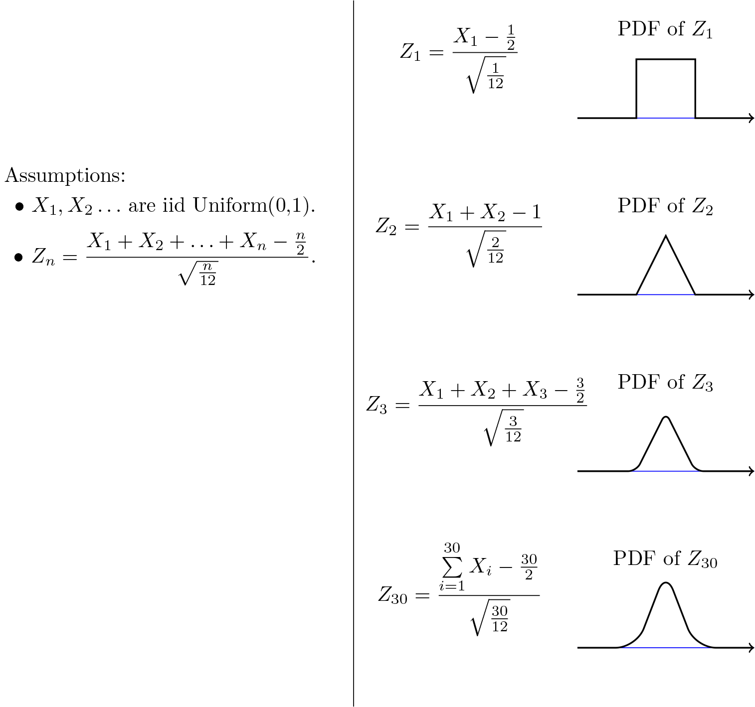
Fig. 7.2 -
Zn
Z
n
is the normalized sum of
n
n
independent
Uniform(0,1)
U
n
i
f
o
r
m
(
0
,
1
)
random variables. The shape of its PDF,
fZn(z)
f
Z
n
(
z
)
, gets closer to the normal curve as
n
n
increases.
We could have directly looked at Yn\=X1\+X2\+...\+Xn Y n \= X 1 \+ X 2 \+ . . . \+ X n, so why do we normalize it first and say that the normalized version (Zn Z n) becomes approximately normal? This is because EYn\=nEXi E Y n \= n E X i and Var(Yn)\=nσ2 V a r ( Y n ) \= n σ 2 go to infinity as n n goes to infinity. We normalize Yn Y n in order to have a finite mean and variance (EZn\=0 E Z n \= 0, Var(Zn)\=1 V a r ( Z n ) \= 1). Nevertheless, for any fixed n n, the CDF of Zn Z n is obtained by scaling and shifting the CDF of Yn Y n. Thus, the two CDFs have similar shapes.
The importance of the central limit theorem stems from the fact that, in many real applications, a certain random variable of interest is a sum of a large number of independent random variables. In these situations, we are often able to use the CLT to justify using the normal distribution. Examples of such random variables are found in almost every discipline. Here are a few:
- Laboratory measurement errors are usually modeled by normal random variables.
- In communication and signal processing, Gaussian noise is the most frequently used model for noise.
- In finance, the percentage changes in the prices of some assets are sometimes modeled by normal random variables.
- When we do random sampling from a population to obtain statistical knowledge about the population, we often model the resulting quantity as a normal random variable.
The CLT is also very useful in the sense that it can simplify our computations significantly. If you have a problem in which you are interested in a sum of one thousand i.i.d. random variables, it might be extremely difficult, if not impossible, to find the distribution of the sum by direct calculation. Using the CLT we can immediately write the distribution, if we know the mean and variance of the Xi X i's.
Another question that comes to mind is how large n n should be so that we can use the normal approximation. The answer generally depends on the distribution of the Xi X is. Nevertheless, as a rule of thumb it is often stated that if n n is larger than or equal to 30 30, then the normal approximation is very good.
Let's summarize how we use the CLT to solve problems:
How to Apply The Central Limit Theorem (CLT)
Here are the steps that we need in order to apply the CLT:
1. Write the random variable of interest,
Y
Y
, as the sum of
n
n
i.i.d. random variable
Xi
X
i
's:
Y\=X1\+X2\+...\+Xn.
Y
\=
X
1
\+
X
2
\+
.
.
.
\+
X
n
.
2. Find
EY
E
Y
and
Var(Y)
V
a
r
(
Y
)
by noting that
EY\=nμ,Var(Y)\=nσ2,
E
Y
\=
n
μ
,
V
a
r
(
Y
)
\=
n
σ
2
,
where
μ\=EXi
μ
\=
E
X
i
and
σ2\=Var(Xi)
σ
2
\=
V
a
r
(
X
i
)
.
3. According to the CLT, conclude that
Y−EYVar(Y)√\=Y−nμn√σ
Y
−
E
Y
V
a
r
(
Y
)
\=
Y
−
n
μ
n
σ
is approximately standard normal; thus, to find
P(y1≤Y≤y2)
P
(
y
1
≤
Y
≤
y
2
)
, we can write
P(y1≤Y≤y2)\=P(y1−nμn−−√σ≤Y−nμn−−√σ≤y2−nμn−−√σ)≈Φ(y2−nμn−−√σ)−Φ(y1−nμn−−√σ).
P
(
y
1
≤
Y
≤
y
2
)
\=
P
(
y
1
−
n
μ
n
σ
≤
Y
−
n
μ
n
σ
≤
y
2
−
n
μ
n
σ
)
≈
Φ
(
y
2
−
n
μ
n
σ
)
−
Φ
(
y
1
−
n
μ
n
σ
)
.
Let us look at some examples to see how we can use the central limit theorem.
***
Example
A bank teller serves customers standing in the queue one by one. Suppose that the service time Xi X i for customer i i has mean EXi\=2 E X i \= 2 (minutes) and Var(Xi)\=1 V a r ( X i ) \= 1. We assume that service times for different bank customers are independent. Let Y Y be the total time the bank teller spends serving 50 50 customers. Find P(90\<Y\<110) P ( 90 \< Y \< 110 ).
- [**Solution**]()
- Y\=X1\+X2\+...\+Xn,
Y
\=
X
1
\+
X
2
\+
.
.
.
\+
X
n
,
where
n\=50
n
\=
50
,
EXi\=μ\=2
E
X
i
\=
μ
\=
2
, and
Var(Xi)\=σ2\=1
V
a
r
(
X
i
)
\=
σ
2
\=
1
. Thus, we can write
P(90\<Y≤110)\=P(90−nμn−−√σ\<Y−nμn−−√σ\<110−nμn−−√σ)\=P(90−10050−−√\<Y−nμn−−√σ\<110−10050−−√)\=P(−2–√\<Y−nμn−−√σ\<2–√).
P
(
90
\<
Y
≤
110
)
\=
P
(
90
−
n
μ
n
σ
\<
Y
−
n
μ
n
σ
\<
110
−
n
μ
n
σ
)
\=
P
(
90
−
100
50
\<
Y
−
n
μ
n
σ
\<
110
−
100
50
)
\=
P
(
−
2
\<
Y
−
n
μ
n
σ
\<
2
)
.
By the CLT,
Y−nμn√σ
Y
−
n
μ
n
σ
is approximately standard normal, so we can write
P(90\<Y≤110)≈Φ(2–√)−Φ(−2–√)\=0\.8427
P
(
90
\<
Y
≤
110
)
≈
Φ
(
2
)
−
Φ
(
−
2
)
\=
0\.8427
***
Example
In a communication system each data packet consists of 1000 1000 bits. Due to the noise, each bit may be received in error with probability 0\.1 0\.1. It is assumed bit errors occur independently. Find the probability that there are more than 120 120 errors in a certain data packet.
- [**Solution**]()
- Let us define Xi X i as the indicator random variable for the i ith bit in the packet. That is, Xi\=1 X i \= 1 if the i ith bit is received in error, and Xi\=0 X i \= 0 otherwise. Then the Xi X i's are i.i.d. and Xi∼Bernoulli(p\=0\.1) X i ∼ B e r n o u l l i ( p \= 0\.1 ). If Y Y is the total number of bit errors in the packet, we have
Y\=X1\+X2\+...\+Xn.
Y
\=
X
1
\+
X
2
\+
.
.
.
\+
X
n
.
Since
Xi∼Bernoulli(p\=0\.1)
X
i
∼
B
e
r
n
o
u
l
l
i
(
p
\=
0\.1
)
, we have
EXi\=μ\=p\=0\.1,Var(Xi)\=σ2\=p(1−p)\=0\.09
E
X
i
\=
μ
\=
p
\=
0\.1
,
V
a
r
(
X
i
)
\=
σ
2
\=
p
(
1
−
p
)
\=
0\.09
Using the CLT, we have
P(Y\>120)\=P(Y−nμn−−√σ\>120−nμn−−√σ)\=P(Y−nμn−−√σ\>120−10090−−√)≈1−Φ(2090−−√)\=0\.0175
P
(
Y
\>
120
)
\=
P
(
Y
−
n
μ
n
σ
\>
120
−
n
μ
n
σ
)
\=
P
(
Y
−
n
μ
n
σ
\>
120
−
100
90
)
≈
1
−
Φ
(
20
90
)
\=
0\.0175
***
**Continuity Correction:**
Let us assume that Y∼Binomial(n\=20,p\=12) Y ∼ B i n o m i a l ( n \= 20 , p \= 1 2 ), and suppose that we are interested in P(8≤Y≤10) P ( 8 ≤ Y ≤ 10 ). We know that a Binomial(n\=20,p\=12) B i n o m i a l ( n \= 20 , p \= 1 2 ) can be written as the sum of n n i.i.d. Bernoulli(p) B e r n o u l l i ( p ) random variables:
Y\=X1\+X2\+...\+Xn.
Y
\=
X
1
\+
X
2
\+
.
.
.
\+
X
n
.
Since
Xi∼Bernoulli(p\=12)
X
i
∼
B
e
r
n
o
u
l
l
i
(
p
\=
1
2
)
, we have
EXi\=μ\=p\=12,Var(Xi)\=σ2\=p(1−p)\=14.
E
X
i
\=
μ
\=
p
\=
1
2
,
V
a
r
(
X
i
)
\=
σ
2
\=
p
(
1
−
p
)
\=
1
4
.
Thus, we may want to apply the CLT to write
P(8≤Y≤10)\=P(8−nμn−−√σ\<Y−nμn−−√σ\<10−nμn−−√σ)\=P(8−105–√\<Y−nμn−−√σ\<10−105–√)≈Φ(0)−Φ(−25–√)\=0\.3145
P
(
8
≤
Y
≤
10
)
\=
P
(
8
−
n
μ
n
σ
\<
Y
−
n
μ
n
σ
\<
10
−
n
μ
n
σ
)
\=
P
(
8
−
10
5
\<
Y
−
n
μ
n
σ
\<
10
−
10
5
)
≈
Φ
(
0
)
−
Φ
(
−
2
5
)
\=
0\.3145
Since, here, n\=20 n \= 20 is relatively small, we can actually find P(8≤Y≤10) P ( 8 ≤ Y ≤ 10 ) accurately. We have
P(8≤Y≤10)\=∑k\=810(nk)pk(1−p)n−k\=\[(208)\+(209)\+(2010)\](12)20\=0\.4565
P
(
8
≤
Y
≤
10
)
\=
∑
k
\=
8
10
(
n
k
)
p
k
(
1
−
p
)
n
−
k
\=
\[
(
20
8
)
\+
(
20
9
)
\+
(
20
10
)
\]
(
1
2
)
20
\=
0\.4565
We notice that our approximation is not so good. Part of the error is due to the fact that Y Y is a discrete random variable and we are using a continuous distribution to find P(8≤Y≤10) P ( 8 ≤ Y ≤ 10 ). Here is a trick to get a better approximation, called **continuity correction**. Since Y Y can only take integer values, we can write
P(8≤Y≤10)\=P(7\.5\<Y\<10\.5)\=P(7\.5−nμn−−√σ\<Y−nμn−−√σ\<10\.5−nμn−−√σ)\=P(7\.5−105–√\<Y−nμn−−√σ\<10\.5−105–√)≈Φ(0\.55–√)−Φ(−2\.55–√)\=0\.4567
P
(
8
≤
Y
≤
10
)
\=
P
(
7\.5
\<
Y
\<
10\.5
)
\=
P
(
7\.5
−
n
μ
n
σ
\<
Y
−
n
μ
n
σ
\<
10\.5
−
n
μ
n
σ
)
\=
P
(
7\.5
−
10
5
\<
Y
−
n
μ
n
σ
\<
10\.5
−
10
5
)
≈
Φ
(
0\.5
5
)
−
Φ
(
−
2\.5
5
)
\=
0\.4567
As we see, using continuity correction, our approximation improved significantly. The continuity correction is particularly useful when we would like to find P(y1≤Y≤y2) P ( y 1 ≤ Y ≤ y 2 ), where Y Y is binomial and y1 y 1 and y2 y 2 are close to each other.
Continuity Correction for Discrete Random Variables
Let X1 X 1,X2 X 2, ⋯ ⋯,Xn X n be independent discrete random variables and let
Y\=X1\+X2\+⋯\+Xn.
Y
\=
X
1
\+
X
2
\+
⋯
\+
X
n
.
Suppose that we are interested in finding
P(A)\=P(l≤Y≤u)
P
(
A
)
\=
P
(
l
≤
Y
≤
u
)
using the CLT, where
l
l
and
u
u
are integers. Since
Y
Y
is an integer-valued random variable, we can write
P(A)\=P(l−12≤Y≤u\+12).
P
(
A
)
\=
P
(
l
−
1
2
≤
Y
≤
u
\+
1
2
)
.
It turns out that the above expression sometimes provides a better approximation for P(A) P ( A ) when applying the CLT. This is called the continuity correction and it is particularly useful when Xi X i's are Bernoulli (i.e., Y Y is binomial).
***
[←]() [previous](https://www.probabilitycourse.com/chapter7/chapter7/7_1_1_law_of_large_numbers.php)
[next](https://www.probabilitycourse.com/chapter7/chapter7/7_1_3_solved_probs.php) [→]()
***
| |
|---|
| The print version of the book is available on [Amazon](https://www.amazon.com/Introduction-Probability-Statistics-Random-Processes/dp/0990637204/ref=sr_1_1?ie=UTF8&qid=1408880878&sr=8-1&keywords=pishro-nik). [](https://www.amazon.com/Introduction-Probability-Statistics-Random-Processes/dp/0990637204/ref=sr_1_1?ie=UTF8&qid=1408880878&sr=8-1&keywords=pishro-nik) |
| **Practical uncertainty:** *Useful Ideas in Decision-Making, Risk, Randomness, & AI* [](https://www.amazon.com/dp/B0CH2BHRVH/ref=tmm_pap_swatch_0?_encoding=UTF8&qid=1693837152&sr=8-1) |
Open Menu
- [0 Preface](https://www.probabilitycourse.com/preface.php)
- [1 Basic Concepts]()
- [1\.0 Introduction](https://www.probabilitycourse.com/chapter1/1_0_0_introduction.php)
- [1\.1 Introduction]()
- [1\.1.0 What Is Probability?](https://www.probabilitycourse.com/chapter1/1_1_0_what_is_probability.php)
- [1\.1.1 Example](https://www.probabilitycourse.com/chapter1/1_1_1_example.php)
- [1\.2 Review of Set Theory]()
- [1\.2.0 Review](https://www.probabilitycourse.com/chapter1/1_2_0_review_set_theory.php)
- [1\.2.1 Venn Diagrams](https://www.probabilitycourse.com/chapter1/1_2_1_venn.php)
- [1\.2.2 Set Operations](https://www.probabilitycourse.com/chapter1/1_2_2_set_operations.php)
- [1\.2.3 Cardinality](https://www.probabilitycourse.com/chapter1/1_2_3_cardinality.php)
- [1\.2.4 Functions](https://www.probabilitycourse.com/chapter1/1_2_4_functions.php)
- [1\.2.5 Solved Problems](https://www.probabilitycourse.com/chapter1/1_2_5_solved1.php)
- [1\.3 Random Experiments and Probabilities]()
- [1\.3.1 Random Experiments](https://www.probabilitycourse.com/chapter1/1_3_1_random_experiments.php)
- [1\.3.2 Probability](https://www.probabilitycourse.com/chapter1/1_3_2_probability.php)
- [1\.3.3 Finding Probabilities](https://www.probabilitycourse.com/chapter1/1_3_3_finding_probabilities.php)
- [1\.3.4 Discrete Models](https://www.probabilitycourse.com/chapter1/1_3_4_discrete_models.php)
- [1\.3.5 Continuous Models](https://www.probabilitycourse.com/chapter1/1_3_5_continuous_models.php)
- [1\.3.6 Solved Problems](https://www.probabilitycourse.com/chapter1/1_3_6_solved2.php)
- [1\.4 Conditional Probability]()
- [1\.4.0 Conditional Probability](https://www.probabilitycourse.com/chapter1/1_4_0_conditional_probability.php)
- [1\.4.1 Independence](https://www.probabilitycourse.com/chapter1/1_4_1_independence.php)
- [1\.4.2 Law of Total Probability](https://www.probabilitycourse.com/chapter1/1_4_2_total_probability.php)
- [1\.4.3 Bayes' Rule](https://www.probabilitycourse.com/chapter1/1_4_3_bayes_rule.php)
- [1\.4.4 Conditional Independence](https://www.probabilitycourse.com/chapter1/1_4_4_conditional_independence.php)
- [1\.4.5 Solved Problems](https://www.probabilitycourse.com/chapter1/1_4_5_solved3.php)
- [1\.5 Problems]()
- [1\.5.0 End of Chapter Problems](https://www.probabilitycourse.com/chapter1/1_5_0_chapter1_problems.php)
- [2 Combinatorics: Counting Methods]()
- [2\.1 Combinatorics]()
- [2\.1.0 Finding Probabilities with Counting Methods](https://www.probabilitycourse.com/chapter2/2_1_0_counting.php)
- [2\.1.1 Ordered with Replacement](https://www.probabilitycourse.com/chapter2/2_1_1_ordered_with_replacement.php)
- [2\.1.2 Ordered without Replacement](https://www.probabilitycourse.com/chapter2/2_1_2_ordered_without_replacement.php)
- [2\.1.3 Unordered without Replacement](https://www.probabilitycourse.com/chapter2/2_1_3_unordered_without_replacement.php)
- [2\.1.4 Unordered with Replacement](https://www.probabilitycourse.com/chapter2/2_1_4_unordered_with_replacement.php)
- [2\.1.5 Solved Problems](https://www.probabilitycourse.com/chapter2/2_1_5_solved2_1.php)
- [2\.2 Problems]()
- [2\.2.0 End of Chapter Problems](https://www.probabilitycourse.com/chapter2/2_3_0_chapter2_problems.php)
- [3 Discrete Random Variables]()
- [3\.1 Basic Concepts]()
- [3\.1.1 Random Variables](https://www.probabilitycourse.com/chapter3/3_1_1_random_variables.php)
- [3\.1.2 Discrete Random Variables](https://www.probabilitycourse.com/chapter3/3_1_2_discrete_random_var.php)
- [3\.1.3 Probability Mass Function](https://www.probabilitycourse.com/chapter3/3_1_3_pmf.php)
- [3\.1.4 Independent Random Variables](https://www.probabilitycourse.com/chapter3/3_1_4_independent_random_var.php)
- [3\.1.5 Special Distributions](https://www.probabilitycourse.com/chapter3/3_1_5_special_discrete_distr.php)
- [3\.1.6 Solved Problems](https://www.probabilitycourse.com/chapter3/3_1_6_solved3_1.php)
- [3\.2 More about Discrete Random Variables]()
- [3\.2.1 Cumulative Distribution Function](https://www.probabilitycourse.com/chapter3/3_2_1_cdf.php)
- [3\.2.2 Expectation](https://www.probabilitycourse.com/chapter3/3_2_2_expectation.php)
- [3\.2.3 Functions of Random Variables](https://www.probabilitycourse.com/chapter3/3_2_3_functions_random_var.php)
- [3\.2.4 Variance](https://www.probabilitycourse.com/chapter3/3_2_4_variance.php)
- [3\.2.5 Solved Problems](https://www.probabilitycourse.com/chapter3/3_2_5_solved3_2.php)
- [3\.3 Problems]()
- [3\.3.0 End of Chapter Problems](https://www.probabilitycourse.com/chapter3/3_3_0_chapter3_problems.php)
- [4 Continuous and Mixed Random Variables]()
- [4\.0 Introduction](https://www.probabilitycourse.com/chapter4/4_0_0_intro.php)
- [4\.1 Continuous Random Variables]()
- [4\.1.0 Continuous Random Variables and their Distributions](https://www.probabilitycourse.com/chapter4/4_1_0_continuous_random_vars_distributions.php)
- [4\.1.1 Probability Density Function](https://www.probabilitycourse.com/chapter4/4_1_1_pdf.php)
- [4\.1.2 Expected Value and Variance](https://www.probabilitycourse.com/chapter4/4_1_2_expected_val_variance.php)
- [4\.1.3 Functions of Continuous Random Variables](https://www.probabilitycourse.com/chapter4/4_1_3_functions_continuous_var.php)
- [4\.1.4 Solved Problems](https://www.probabilitycourse.com/chapter4/4_1_4_solved4_1.php)
- [4\.2 Special Distributions]()
- [4\.2.1 Uniform Distribution](https://www.probabilitycourse.com/chapter4/4_2_1_uniform.php)
- [4\.2.2 Exponential Distribution](https://www.probabilitycourse.com/chapter4/4_2_2_exponential.php)
- [4\.2.3 Normal (Gaussian) Distribution](https://www.probabilitycourse.com/chapter4/4_2_3_normal.php)
- [4\.2.4 Gamma Distribution](https://www.probabilitycourse.com/chapter4/4_2_4_Gamma_distribution.php)
- [4\.2.5 Other Distributions](https://www.probabilitycourse.com/chapter4/4_2_5_other_distr.php)
- [4\.2.6 Solved Problems](https://www.probabilitycourse.com/chapter4/4_2_6_solved4_2.php)
- [4\.3 Mixed Random Variables]()
- [4\.3.1 Mixed Random Variables](https://www.probabilitycourse.com/chapter4/4_3_1_mixed.php)
- [4\.3.2 Using the Delta Function](https://www.probabilitycourse.com/chapter4/4_3_2_delta_function.php)
- [4\.3.3 Solved Problems](https://www.probabilitycourse.com/chapter4/4_3_3_solved4_3.php)
- [4\.4 Problems]()
- [4\.4.0 End of Chapter Problems](https://www.probabilitycourse.com/chapter4/4_4_0_chapter4_problems.php)
- [5 Joint Distributions]()
- [5\.1 Two Discrete Random Variables]()
- [5\.1.0 Two Random Variables](https://www.probabilitycourse.com/chapter5/5_1_0_joint_distributions.php)
- [5\.1.1 Joint Probability Mass Function (PMF)](https://www.probabilitycourse.com/chapter5/5_1_1_joint_pmf.php)
- [5\.1.2 Joint Cumulative Distribution Function (CDF)](https://www.probabilitycourse.com/chapter5/5_1_2_joint_cdf.php)
- [5\.1.3 Conditioning and Independence](https://www.probabilitycourse.com/chapter5/5_1_3_conditioning_independence.php)
- [5\.1.4 Functions of Two Random Variables](https://www.probabilitycourse.com/chapter5/5_1_4_functions_two_variables.php)
- [5\.1.5 Conditional Expectation](https://www.probabilitycourse.com/chapter5/5_1_5_conditional_expectation.php)
- [5\.1.6 Solved Problems](https://www.probabilitycourse.com/chapter5/5_1_6_solved_prob.php)
- [5\.2 Two Continuous Random Variables]()
- [5\.2.0 Two Continuous Random Variables](https://www.probabilitycourse.com/chapter5/5_2_0_continuous_vars.php)
- [5\.2.1 Joint Probability Density Function](https://www.probabilitycourse.com/chapter5/5_2_1_joint_pdf.php)
- [5\.2.2 Joint Cumulative Distribution Function](https://www.probabilitycourse.com/chapter5/5_2_2_joint_cdf.php)
- [5\.2.3 Conditioning and Independence](https://www.probabilitycourse.com/chapter5/5_2_3_conditioning_independence.php)
- [5\.2.4 Functions of Two Continuous Random Variables](https://www.probabilitycourse.com/chapter5/5_2_4_functions.php)
- [5\.2.5 Solved Problems](https://www.probabilitycourse.com/chapter5/5_2_5_solved_prob.php)
- [5\.3 More Topics]()
- [5\.3.1 Covariance and Correlation](https://www.probabilitycourse.com/chapter5/5_3_1_covariance_correlation.php)
- [5\.3.2 Bivariate Normal Distribution](https://www.probabilitycourse.com/chapter5/5_3_2_bivariate_normal_dist.php)
- [5\.3.3 Solved Problems](https://www.probabilitycourse.com/chapter5/5_3_3_solved_probs.php)
- [5\.4 Problems]()
- [5\.4.0 End of Chapter Problems](https://www.probabilitycourse.com/chapter5/5_4_0_chapter_problems.php)
- [6 Multiple Random Variables]()
- [6\.0 Introduction](https://www.probabilitycourse.com/chapter6/6_0_0_intro.php)
- [6\.1 Methods for More Than Two Random Variables]()
- [6\.1.1 Joint Distributions and Independence](https://www.probabilitycourse.com/chapter6/6_1_1_joint_distributions_independence.php)
- [6\.1.2 Sums of Random Variables](https://www.probabilitycourse.com/chapter6/6_1_2_sums_random_variables.php)
- [6\.1.3 Moment Generating Functions](https://www.probabilitycourse.com/chapter6/6_1_3_moment_functions.php)
- [6\.1.4 Characteristic Functions](https://www.probabilitycourse.com/chapter6/6_1_4_characteristic_functions.php)
- [6\.1.5 Random Vectors](https://www.probabilitycourse.com/chapter6/6_1_5_random_vectors.php)
- [6\.1.6 Solved Problems](https://www.probabilitycourse.com/chapter6/6_1_6_solved_probs.php)
- [6\.2 Probability Bounds]()
- [6\.2.0 Probability Bounds](https://www.probabilitycourse.com/chapter6/6_2_0_probability_bounds.php)
- [6\.2.1 Union Bound and Extension](https://www.probabilitycourse.com/chapter6/6_2_1_union_bound_and_exten.php)
- [6\.2.2 Markov Chebyshev Inequalities](https://www.probabilitycourse.com/chapter6/6_2_2_markov_chebyshev_inequalities.php)
- [6\.2.3 Chernoff Bounds](https://www.probabilitycourse.com/chapter6/6_2_3_chernoff_bounds.php)
- [6\.2.4 Cauchy Schwarz Inequality](https://www.probabilitycourse.com/chapter6/6_2_4_cauchy_schwarz.php)
- [6\.2.5 Jensen's Inequality](https://www.probabilitycourse.com/chapter6/6_2_5_jensen's_inequality.php)
- [6\.2.6 Solved Problems](https://www.probabilitycourse.com/chapter6/6_2_6_solved6_2.php)
- [6\.3 Problems]()
- [6\.3.0 End of Chapter Problems](https://www.probabilitycourse.com/chapter6/6_3_0_chapter_problems.php)
- [7 Limit Theorems and Convergence of Random Variables]()
- [7\.0 Introduction](https://www.probabilitycourse.com/chapter7/7_0_0_intro.php)
- [7\.1 Limit Theorems]()
- [7\.1.0 Limit Theorems](https://www.probabilitycourse.com/chapter7/7_1_0_limit_theorems.php)
- [7\.1.1 Law of Large Numbers](https://www.probabilitycourse.com/chapter7/7_1_1_law_of_large_numbers.php)
- [7\.1.2 Central Limit Theorem (CLT)](https://www.probabilitycourse.com/chapter7/7_1_2_central_limit_theorem.php)
- [7\.1.3 Solved Problems](https://www.probabilitycourse.com/chapter7/7_1_3_solved_probs.php)
- [7\.2 Convergence of Random Variables]()
- [7\.2.0 Convergence of Random Variables](https://www.probabilitycourse.com/chapter7/7_2_0_convergence_of_random_variables.php)
- [7\.2.1 Convergence of Sequence of Numbers](https://www.probabilitycourse.com/chapter7/7_2_1_convergence_of_a_seq_of_nums.php)
- [7\.2.2 Sequence of Random Variables](https://www.probabilitycourse.com/chapter7/7_2_2_sequence_of_random_variables.php)
- [7\.2.3 Different Types of Convergence for Sequences of Random Variables](https://www.probabilitycourse.com/chapter7/7_2_3_different_types_of_convergence_for_sequences_of_random_variables.php)
- [7\.2.4 Convergence in Distribution](https://www.probabilitycourse.com/chapter7/7_2_4_convergence_in_distribution.php)
- [7\.2.5 Convergence in Probability](https://www.probabilitycourse.com/chapter7/7_2_5_convergence_in_probability.php)
- [7\.2.6 Convergence in Mean](https://www.probabilitycourse.com/chapter7/7_2_6_convergence_in_mean.php)
- [7\.2.7 Almost Sure Convergence](https://www.probabilitycourse.com/chapter7/7_2_7_almost_sure_convergence.php)
- [7\.2.8 Solved Problems](https://www.probabilitycourse.com/chapter7/7_2_8_solved_probs.php)
- [7\.3 Problems]()
- [7\.3.0 End of Chapter Problems](https://www.probabilitycourse.com/chapter7/7_3_0_chapter_problem.php)
- [8 Statistical Inference I: Classical Methods]()
- [8\.1 Introduction]()
- [8\.1.0 Introduction](https://www.probabilitycourse.com/chapter8/8_1_0_intro.php)
- [8\.1.1 Random Sampling](https://www.probabilitycourse.com/chapter8/8_1_1_random_sampling.php)
- [8\.2 Point Estimation]()
- [8\.2.0 Point Estimation](https://www.probabilitycourse.com/chapter8/8_2_0_point_estimation.php)
- [8\.2.1 Evaluating Estimators](https://www.probabilitycourse.com/chapter8/8_2_1_evaluating_estimators.php)
- [8\.2.2 Point Estimators for Mean and Variance](https://www.probabilitycourse.com/chapter8/8_2_2_point_estimators_for_mean_and_var.php)
- [8\.2.3 Maximum Likelihood Estimation (MLE)](https://www.probabilitycourse.com/chapter8/8_2_3_max_likelihood_estimation.php)
- [8\.2.4 Asymptotic Properties of MLEs](https://www.probabilitycourse.com/chapter8/8_2_4_asymptotic_probs_of_MLE.php)
- [8\.2.5 Solved Problems](https://www.probabilitycourse.com/chapter8/8_2_5_solved_probs.php)
- [8\.3 Interval Estimation (Confidence Intervals)]()
- [8\.3.0 Interval Estimation (Confidence Intervals)](https://www.probabilitycourse.com/chapter8/8_3_0_interval_estimation.php)
- [8\.3.1 The general framework of Interval Estimation](https://www.probabilitycourse.com/chapter8/8_3_1_gen_framework_of_int_estimation.php)
- [8\.3.2 Finding Interval Estimators](https://www.probabilitycourse.com/chapter8/8_3_2_finding_interval_estimators.php)
- [8\.3.3 Confidence Intervals for Normal Samples](https://www.probabilitycourse.com/chapter8/8_3_3_confidence_intervals_for_norm_samples.php)
- [8\.3.4 Solved Problems](https://www.probabilitycourse.com/chapter8/8_3_4_solved_probs.php)
- [8\.4 Hypothesis Testing]()
- [8\.4.1 Introduction](https://www.probabilitycourse.com/chapter8/8_4_1_intro.php)
- [8\.4.2 General Setting and Definitions](https://www.probabilitycourse.com/chapter8/8_4_2_general_setting_definitions.php)
- [8\.4.3 Hypothesis Testing for the Mean](https://www.probabilitycourse.com/chapter8/8_4_3_hypothesis_testing_for_mean.php)
- [8\.4.4 P-Values](https://www.probabilitycourse.com/chapter8/8_4_4_p_vals.php)
- [8\.4.5 Likelihood Ratio Tests](https://www.probabilitycourse.com/chapter8/8_4_5_likelihood_ratio_tests.php)
- [8\.4.6 Solved Problems](https://www.probabilitycourse.com/chapter8/8_4_6_solved_probs.php)
- [8\.5 Linear Regression]()
- [8\.5.0 Linear Regression](https://www.probabilitycourse.com/chapter8/8_5_0_linear_regression.php)
- [8\.5.1 Simple Linear Regression Model](https://www.probabilitycourse.com/chapter8/8_5_1_simple_linear_regression_model.php)
- [8\.5.2 The First Method for Finding beta](https://www.probabilitycourse.com/chapter8/8_5_2_first_method_for_finding_beta.php)
- [8\.5.3 The Method of Least Squares](https://www.probabilitycourse.com/chapter8/8_5_3_the_method_of_least_squares.php)
- [8\.5.4 Extensions and Issues](https://www.probabilitycourse.com/chapter8/8_5_4_extensions_and_issues.php)
- [8\.5.5 Solved Problems](https://www.probabilitycourse.com/chapter8/8_5_5_solved_probs.php)
- [8\.6 Problems]()
- [8\.6.0 End of Chapter Problems](https://www.probabilitycourse.com/chapter8/8_6_0_ch_probs.php)
- [9 Statistical Inference II: Bayesian Inference]()
- [9\.1 Bayesian Inference]()
- [9\.1.0 Bayesian Inference](https://www.probabilitycourse.com/chapter9/9_1_0_bayesian_inference.php)
- [9\.1.1 Prior and Posterior](https://www.probabilitycourse.com/chapter9/9_1_1_prior_and_posterior.php)
- [9\.1.2 Maximum A Posteriori (MAP) Estimation](https://www.probabilitycourse.com/chapter9/9_1_2_MAP_estimation.php)
- [9\.1.3 Comparison to ML Estimation](https://www.probabilitycourse.com/chapter9/9_1_3_comparison_to_ML_estimation.php)
- [9\.1.4 Conditional Expectation (MMSE)](https://www.probabilitycourse.com/chapter9/9_1_4_conditional_expectation_MMSE.php)
- [9\.1.5 Mean Squared Error (MSE)](https://www.probabilitycourse.com/chapter9/9_1_5_mean_squared_error_MSE.php)
- [9\.1.6 Linear MMSE Estimation of Random Variables](https://www.probabilitycourse.com/chapter9/9_1_6_linear_MMSE_estimat_of_random_vars.php)
- [9\.1.7 Estimation for Random Vectors](https://www.probabilitycourse.com/chapter9/9_1_7_estimation_for_random_vectors.php)
- [9\.1.8 Bayesian Hypothesis Testing](https://www.probabilitycourse.com/chapter9/9_1_8_bayesian_hypothesis_testing.php)
- [9\.1.9 Bayesian Interval Estimation](https://www.probabilitycourse.com/chapter9/9_1_9_bayesian_interval_estimation.php)
- [9\.1.10 Solved Problems](https://www.probabilitycourse.com/chapter9/9_1_10_solved_probs.php)
- [9\.2 Problems]()
- [9\.2.0 End of Chapter Problems](https://www.probabilitycourse.com/chapter9/9_2_0_ch_probs.php)
- [10 Introduction to Random Processes]()
- [10\.1 Basic Concepts]()
- [10\.1.0 Basic Concepts](https://www.probabilitycourse.com/chapter10/10_1_0_basic_concepts.php)
- [10\.1.1 PDFs and CDFs](https://www.probabilitycourse.com/chapter10/10_1_1_PDFs_and_CDFs.php)
- [10\.1.2 Mean and Correlation Functions](https://www.probabilitycourse.com/chapter10/10_1_2_mean_and_correlation_functions.php)
- [10\.1.3 Multiple Random Processes](https://www.probabilitycourse.com/chapter10/10_1_3_multiple_random_processes.php)
- [10\.1.4 Stationary Processes](https://www.probabilitycourse.com/chapter10/10_1_4_stationary_processes.php)
- [10\.1.5 Gaussian Random Processes](https://www.probabilitycourse.com/chapter10/10_1_5_gaussian_random_processes.php)
- [10\.1.6 Solved Problems](https://www.probabilitycourse.com/chapter10/10_1_6_solved_probs.php)
- [10\.2 Processing of Random Signals]()
- [10\.2.0 Processing of Random Signals](https://www.probabilitycourse.com/chapter10/10_2_0_processing_of_random_signals.php)
- [10\.2.1 Power Spectral Density](https://www.probabilitycourse.com/chapter10/10_2_1_power_spectral_density.php)
- [10\.2.2 Linear Time-Invariant (LTI) Systems with Random Inputs](https://www.probabilitycourse.com/chapter10/10_2_2_LTI_systems_with_random_inputs.php)
- [10\.2.3 Power in a Frequency Band](https://www.probabilitycourse.com/chapter10/10_2_3_power_in_a_frequency_band.php)
- [10\.2.4 White Noise](https://www.probabilitycourse.com/chapter10/10_2_4_white_noise.php)
- [10\.2.5 Solved Problems](https://www.probabilitycourse.com/chapter10/10_2_5_solved_probs.php)
- [10\.3 Problems]()
- [10\.3.0 End of Chapter Problems](https://www.probabilitycourse.com/chapter10/10_3_0_ch_probs.php)
- [11 Some Important Random Processes]()
- [11\.1 Poisson Processes]()
- [11\.1.0 Introduction](https://www.probabilitycourse.com/chapter11/11_0_0_intro.php)
- [11\.1.1 Counting Processes](https://www.probabilitycourse.com/chapter11/11_1_1_counting_processes.php)
- [11\.1.2 Basic Concepts of the Poisson Process](https://www.probabilitycourse.com/chapter11/11_1_2_basic_concepts_of_the_poisson_process.php)
- [11\.1.3 Merging and Splitting Poisson Processes](https://www.probabilitycourse.com/chapter11/11_1_3_merging_and_splitting_poisson_processes.php)
- [11\.1.4 Nonhomogeneous Poisson Processes](https://www.probabilitycourse.com/chapter11/11_1_4_nonhomogeneous_poisson_processes.php)
- [11\.1.5 Solved Problems](https://www.probabilitycourse.com/chapter11/11_1_5_solved_probs.php)
- [11\.2 Discrete-Time Markov Chains]()
- [11\.2.1 Introduction](https://www.probabilitycourse.com/chapter11/11_2_1_introduction.php)
- [11\.2.2 State Transition Matrix and Diagram](https://www.probabilitycourse.com/chapter11/11_2_2_state_transition_matrix_and_diagram.php)
- [11\.2.3 Probability Distributions](https://www.probabilitycourse.com/chapter11/11_2_3_probability_distributions.php)
- [11\.2.4 Classification of States](https://www.probabilitycourse.com/chapter11/11_2_4_classification_of_states.php)
- [11\.2.5 Using the Law of Total Probability with Recursion](https://www.probabilitycourse.com/chapter11/11_2_5_using_the_law_of_total_probability_with_recursion.php)
- [11\.2.6 Stationary and Limiting Distributions](https://www.probabilitycourse.com/chapter11/11_2_6_stationary_and_limiting_distributions.php)
- [11\.2.7 Solved Problems](https://www.probabilitycourse.com/chapter11/11_2_7_solved_probs.php)
- [11\.3 Continuous-Time Markov Chains]()
- [11\.3.1 Introduction](https://www.probabilitycourse.com/chapter11/11_3_1_introduction.php)
- [11\.3.2 Stationary and Limiting Distributions](https://www.probabilitycourse.com/chapter11/11_3_2_stationary_and_limiting_distributions.php)
- [11\.3.3 The Generator Matrix](https://www.probabilitycourse.com/chapter11/11_3_3_the_generator_matrix.php)
- [11\.3.4 Solved Problems](https://www.probabilitycourse.com/chapter11/11_3_4_solved_probs.php)
- [11\.4 Brownian Motion (Wiener Process)]()
- [11\.4.0 Brownian Motion (Wiener Process)](https://www.probabilitycourse.com/chapter11/11_4_0_brownian_motion_wiener_process.php)
- [11\.4.1 Brownian Motion as the Limit of a Symmetric Random Walk](https://www.probabilitycourse.com/chapter11/11_4_1_brownian_motion_as_the_limit_of_a_symmetric_random_walk.php)
- [1\.4.2 Definition and Some Properties](https://www.probabilitycourse.com/chapter11/11_4_2_definition_and_some_properties.php)
- [11\.4.3 Solved Problems](https://www.probabilitycourse.com/chapter11/11_4_3_solved_probs.php)
- [11\.5 Problems]()
- [11\.5.0 End of Chapter Problems](https://www.probabilitycourse.com/chapter11/11_5_0_end_of_chapter_problems.php)
- [12 Introduction to Simulation Using MATLAB](https://www.probabilitycourse.com/chapter12/chapter12.php)
- [13 Introduction to Simulation Using R](https://www.probabilitycourse.com/chapter13/chapter13.php)
- [14 Introduction to Simulation Using Python](https://www.probabilitycourse.com/chapter14/chapter14.php)
- [15 Recursive Methods](https://www.probabilitycourse.com/chapter15/chapter15.php)
- [Appendix]()
- [Some Important Distributions](https://www.probabilitycourse.com/appendix/some_important_distributions.php)
- [Review of the Fourier Transform](https://www.probabilitycourse.com/appendix/review_fourier_transform.php)
- [Bibliography](https://www.probabilitycourse.com/bibliography.php)
[](https://creativecommons.org/licenses/by-nc-nd/3.0/deed.en_US)
Introduction to Probability by [Hossein Pishro-Nik](https://websites.umass.edu/pishro/) is licensed under a [Creative Commons Attribution-NonCommercial-NoDerivs 3.0 Unported License](https://creativecommons.org/licenses/by-nc-nd/3.0/deed.en_US) |
| Readable Markdown | ***
The **central limit theorem (CLT)** is one of the most important results in probability theory. It states that, under certain conditions, the sum of a large number of random variables is approximately normal. Here, we state a version of the CLT that applies to i.i.d. random variables. Suppose that X 1, X 2 , ... , X n are i.i.d. random variables with expected values E X i \= μ \< ∞ and variance V a r ( X i ) \= σ 2 \< ∞. Then as we saw above, the sample mean X ¯ \= X 1 \+ X 2 \+ . . . \+ X n n has mean E X ¯ \= μ and variance V a r ( X ¯ ) \= σ 2 n. Thus, the normalized random variable
Z n \= X ¯ − μ σ / n \= X 1 \+ X 2 \+ . . . \+ X n − n μ n σ
has mean E Z n \= 0 and variance V a r ( Z n ) \= 1. The central limit theorem states that the CDF of Z n converges to the standard normal CDF.
The Central Limit Theorem (CLT)
Let X 1,X 2,...,X n be i.i.d. random variables with expected value E X i \= μ \< ∞ and variance 0 \< V a r ( X i ) \= σ 2 \< ∞. Then, the random variable
Z n \= X ¯ − μ σ / n \= X 1 \+ X 2 \+ . . . \+ X n − n μ n σ
converges in distribution to the standard normal random variable as n goes to infinity, that is
lim n → ∞ P ( Z n ≤ x ) \= Φ ( x ) , for all x ∈ R ,
where Φ ( x ) is the standard normal CDF.
An interesting thing about the CLT is that it does not matter what the distribution of the X i's is. The X i's can be discrete, continuous, or mixed random variables. To get a feeling for the CLT, let us look at some examples. Let's assume that X i's are B e r n o u l l i ( p ). Then E X i \= p, V a r ( X i ) \= p ( 1 − p ). Also, Y n \= X 1 \+ X 2 \+ . . . \+ X n has B i n o m i a l ( n , p ) distribution. Thus,
Z n \= Y n − n p n p ( 1 − p ) ,
where Y n ∼ B i n o m i a l ( n , p ). Figure 7.1 shows the PMF of Z n for different values of n. As you see, the shape of the PMF gets closer to a normal PDF curve as n increases. Here, Z n is a discrete random variable, so mathematically speaking it has a PMF not a PDF. That is why the CLT states that the CDF (not the PDF) of Z n converges to the standard normal CDF. Nevertheless, since PMF and PDF are conceptually similar, the figure is useful in visualizing the convergence to normal distribution.

Fig.7.1 -
Z
n
is the normalized sum of
n
independent
B
e
r
n
o
u
l
l
i
(
p
)
random variables. The shape of its PMF,
P
Z
n
(
z
)
, resembles the normal curve as
n
increases.
As another example, let's assume that X i's are U n i f o r m ( 0 , 1 ). Then E X i \= 1 2, V a r ( X i ) \= 1 12. In this case,
Z n \= X 1 \+ X 2 \+ . . . \+ X n − n 2 n / 12 .
Figure 7.2 shows the PDF of Z n for different values of n. As you see, the shape of the PDF gets closer to the normal PDF as n increases.

Fig. 7.2 -
Z
n
is the normalized sum of
n
independent
U
n
i
f
o
r
m
(
0
,
1
)
random variables. The shape of its PDF,
f
Z
n
(
z
)
, gets closer to the normal curve as
n
increases.
We could have directly looked at Y n \= X 1 \+ X 2 \+ . . . \+ X n, so why do we normalize it first and say that the normalized version (Z n) becomes approximately normal? This is because E Y n \= n E X i and V a r ( Y n ) \= n σ 2 go to infinity as n goes to infinity. We normalize Y n in order to have a finite mean and variance (E Z n \= 0, V a r ( Z n ) \= 1). Nevertheless, for any fixed n, the CDF of Z n is obtained by scaling and shifting the CDF of Y n. Thus, the two CDFs have similar shapes.
The importance of the central limit theorem stems from the fact that, in many real applications, a certain random variable of interest is a sum of a large number of independent random variables. In these situations, we are often able to use the CLT to justify using the normal distribution. Examples of such random variables are found in almost every discipline. Here are a few:
- Laboratory measurement errors are usually modeled by normal random variables.
- In communication and signal processing, Gaussian noise is the most frequently used model for noise.
- In finance, the percentage changes in the prices of some assets are sometimes modeled by normal random variables.
- When we do random sampling from a population to obtain statistical knowledge about the population, we often model the resulting quantity as a normal random variable.
The CLT is also very useful in the sense that it can simplify our computations significantly. If you have a problem in which you are interested in a sum of one thousand i.i.d. random variables, it might be extremely difficult, if not impossible, to find the distribution of the sum by direct calculation. Using the CLT we can immediately write the distribution, if we know the mean and variance of the X i's.
Another question that comes to mind is how large n should be so that we can use the normal approximation. The answer generally depends on the distribution of the X is. Nevertheless, as a rule of thumb it is often stated that if n is larger than or equal to 30, then the normal approximation is very good.
Let's summarize how we use the CLT to solve problems:
How to Apply The Central Limit Theorem (CLT)
Here are the steps that we need in order to apply the CLT:
1. Write the random variable of interest,
Y
, as the sum of
n
i.i.d. random variable
X
i
's:
Y \= X 1 \+ X 2 \+ . . . \+ X n .
2. Find
E
Y
and
V
a
r
(
Y
)
by noting that
E Y \= n μ , V a r ( Y ) \= n σ 2 ,
where
μ
\=
E
X
i
and
σ
2
\=
V
a
r
(
X
i
)
.
3. According to the CLT, conclude that
Y
−
E
Y
V
a
r
(
Y
)
\=
Y
−
n
μ
n
σ
is approximately standard normal; thus, to find
P
(
y
1
≤
Y
≤
y
2
)
, we can write
P ( y 1 ≤ Y ≤ y 2 ) \= P ( y 1 − n μ n σ ≤ Y − n μ n σ ≤ y 2 − n μ n σ ) ≈ Φ ( y 2 − n μ n σ ) − Φ ( y 1 − n μ n σ ) .
Let us look at some examples to see how we can use the central limit theorem.
***
Example
A bank teller serves customers standing in the queue one by one. Suppose that the service time X i for customer i has mean E X i \= 2 (minutes) and V a r ( X i ) \= 1. We assume that service times for different bank customers are independent. Let Y be the total time the bank teller spends serving 50 customers. Find P ( 90 \< Y \< 110 ).
- [**Solution**]()
- Y \= X 1 \+ X 2 \+ . . . \+ X n ,
where
n
\=
50
,
E
X
i
\=
μ
\=
2
, and
V
a
r
(
X
i
)
\=
σ
2
\=
1
. Thus, we can write
P ( 90 \< Y ≤ 110 ) \= P ( 90 − n μ n σ \< Y − n μ n σ \< 110 − n μ n σ ) \= P ( 90 − 100 50 \< Y − n μ n σ \< 110 − 100 50 ) \= P ( − 2 \< Y − n μ n σ \< 2 ) .
By the CLT,
Y
−
n
μ
n
σ
is approximately standard normal, so we can write
P ( 90 \< Y ≤ 110 ) ≈ Φ ( 2 ) − Φ ( − 2 ) \= 0\.8427
***
Example
In a communication system each data packet consists of 1000 bits. Due to the noise, each bit may be received in error with probability 0\.1. It is assumed bit errors occur independently. Find the probability that there are more than 120 errors in a certain data packet.
- [**Solution**]()
- Let us define X i as the indicator random variable for the ith bit in the packet. That is, X i \= 1 if the ith bit is received in error, and X i \= 0 otherwise. Then the X i's are i.i.d. and X i ∼ B e r n o u l l i ( p \= 0\.1 ). If Y is the total number of bit errors in the packet, we have
Y \= X 1 \+ X 2 \+ . . . \+ X n .
Since
X
i
∼
B
e
r
n
o
u
l
l
i
(
p
\=
0\.1
)
, we have
E X i \= μ \= p \= 0\.1 , V a r ( X i ) \= σ 2 \= p ( 1 − p ) \= 0\.09
Using the CLT, we have
P ( Y \> 120 ) \= P ( Y − n μ n σ \> 120 − n μ n σ ) \= P ( Y − n μ n σ \> 120 − 100 90 ) ≈ 1 − Φ ( 20 90 ) \= 0\.0175
***
**Continuity Correction:**
Let us assume that Y ∼ B i n o m i a l ( n \= 20 , p \= 1 2 ), and suppose that we are interested in P ( 8 ≤ Y ≤ 10 ). We know that a B i n o m i a l ( n \= 20 , p \= 1 2 ) can be written as the sum of n i.i.d. B e r n o u l l i ( p ) random variables:
Y \= X 1 \+ X 2 \+ . . . \+ X n .
Since X i ∼ B e r n o u l l i ( p \= 1 2 ), we have
E X i \= μ \= p \= 1 2 , V a r ( X i ) \= σ 2 \= p ( 1 − p ) \= 1 4 .
Thus, we may want to apply the CLT to write
P ( 8 ≤ Y ≤ 10 ) \= P ( 8 − n μ n σ \< Y − n μ n σ \< 10 − n μ n σ ) \= P ( 8 − 10 5 \< Y − n μ n σ \< 10 − 10 5 ) ≈ Φ ( 0 ) − Φ ( − 2 5 ) \= 0\.3145
Since, here, n \= 20 is relatively small, we can actually find P ( 8 ≤ Y ≤ 10 ) accurately. We have
P ( 8 ≤ Y ≤ 10 ) \= ∑ k \= 8 10 ( n k ) p k ( 1 − p ) n − k \= \[ ( 20 8 ) \+ ( 20 9 ) \+ ( 20 10 ) \] ( 1 2 ) 20 \= 0\.4565
We notice that our approximation is not so good. Part of the error is due to the fact that Y is a discrete random variable and we are using a continuous distribution to find P ( 8 ≤ Y ≤ 10 ). Here is a trick to get a better approximation, called **continuity correction**. Since Y can only take integer values, we can write
P ( 8 ≤ Y ≤ 10 ) \= P ( 7\.5 \< Y \< 10\.5 ) \= P ( 7\.5 − n μ n σ \< Y − n μ n σ \< 10\.5 − n μ n σ ) \= P ( 7\.5 − 10 5 \< Y − n μ n σ \< 10\.5 − 10 5 ) ≈ Φ ( 0\.5 5 ) − Φ ( − 2\.5 5 ) \= 0\.4567
As we see, using continuity correction, our approximation improved significantly. The continuity correction is particularly useful when we would like to find P ( y 1 ≤ Y ≤ y 2 ), where Y is binomial and y 1 and y 2 are close to each other.
Continuity Correction for Discrete Random Variables
Let X 1,X 2, ⋯,X n be independent discrete random variables and let
Y \= X 1 \+ X 2 \+ ⋯ \+ X n .
Suppose that we are interested in finding P ( A ) \= P ( l ≤ Y ≤ u ) using the CLT, where l and u are integers. Since Y is an integer-valued random variable, we can write
P ( A ) \= P ( l − 1 2 ≤ Y ≤ u \+ 1 2 ) .
It turns out that the above expression sometimes provides a better approximation for P ( A ) when applying the CLT. This is called the continuity correction and it is particularly useful when X i's are Bernoulli (i.e., Y is binomial).
***
***
| |
|---|
| The print version of the book is available on [Amazon](https://www.amazon.com/Introduction-Probability-Statistics-Random-Processes/dp/0990637204/ref=sr_1_1?ie=UTF8&qid=1408880878&sr=8-1&keywords=pishro-nik). [](https://www.amazon.com/Introduction-Probability-Statistics-Random-Processes/dp/0990637204/ref=sr_1_1?ie=UTF8&qid=1408880878&sr=8-1&keywords=pishro-nik) |
| **Practical uncertainty:** *Useful Ideas in Decision-Making, Risk, Randomness, & AI* [](https://www.amazon.com/dp/B0CH2BHRVH/ref=tmm_pap_swatch_0?_encoding=UTF8&qid=1693837152&sr=8-1) | |
| Shard | 115 (laksa) |
| Root Hash | 8531609719846996715 |
| Unparsed URL | com,probabilitycourse!www,/chapter7/7_1_2_central_limit_theorem.php s443 |