ℹ️ Skipped - page is already crawled
| Filter | Status | Condition | Details |
|---|---|---|---|
| HTTP status | PASS | download_http_code = 200 | HTTP 200 |
| Age cutoff | PASS | download_stamp > now() - 6 MONTH | 1 months ago |
| History drop | PASS | isNull(history_drop_reason) | No drop reason |
| Spam/ban | PASS | fh_dont_index != 1 AND ml_spam_score = 0 | ml_spam_score=0 |
| Canonical | PASS | meta_canonical IS NULL OR = '' OR = src_unparsed | Not set |
| Property | Value |
|---|---|
| URL | https://www.mdpi.com/1911-8074/13/6/125 |
| Last Crawled | 2026-03-25 01:07:23 (28 days ago) |
| First Indexed | 2020-06-13 15:06:39 (5 years ago) |
| HTTP Status Code | 200 |
| Content | |
| Meta Title | Realized Measures to Explain Volatility Changes over Time |
| Meta Description | We studied (i) the volatility feedback effect, defined as the relationship between contemporaneous returns and the market-based volatility, and (ii) the leverage effect, defined as the relationship between lagged returns and the current market-based volatility. For our analysis, we used daily measures of volatility estimated from high frequency data to explain volatility changes over time for both the S&P500 and FTSE100 indices. The period of analysis spanned from January 2000 to June 2017 incorporating various market phases, such as booms and crashes. Based on the estimated regressions, we found evidence that the returns of S&P500 and FTSE100 indices were well explained by a specific group of realized measure estimators, and the returns negatively affected realized volatility. These results are highly recommended to financial analysts dealing with high frequency data and volatility modelling. |
| Meta Canonical | null |
| Boilerpipe Text | 1. Introduction
Asset pricing in financial literature is predicated on the importance of volatility in asset returns. Hence, financial market volatility is a key factor ranging from investment decisions to derivatives pricing and financial market regulation (
Poon and Granger 2003
). Volatility, as a measure of market risk, is always an anxiety-generating factor for market participants not only in terms of its nature but also its level (
Giot et al. 2010
). Admittedly, volatility is an unobservable variable and its effects on financial markets are hard to anticipate. This is one of the reasons that asset return volatilities (henceforth, volatility) are of utmost importance to empirical finance. In other words, it remains the ingredient in assessing asset or portfolio risk, playing an important role in asset pricing models which heavily depend on underlying asset return dynamics. Asset management and asset pricing models require the proper volatility modeling of financial assets.
The existing literature has laid emphasis on time-varying volatility suggesting various tools for its modeling (see
Andersen and Bollerslev 1998
;
Andersen et al. 2001a
;
Barndorff-Nielsen and Shephard 2002
,
2004
;
Andersen et al. 2007
;
Barndorff-Nielsen et al. 2008
;
Hansen and Horel 2009
;
Meddahi et al. 2011
;
Alghalith et al. 2020
; among others).
Andersen and Bollerslev
(
1998
) showed that ARCH models produce strikingly accurate inter-daily forecasts for the latent volatility on most financial applications.
Andersen et al.
(
2001a
) found evidence that realized volatilities and correlations move together in a manner broadly consistent with latent factor structure.
Barndorff-Nielsen and Shephard
(
2002
) used quadratic variation-like measures of activity in financial markets, called realized volatility, to investigate the stochastic properties of returns.
Barndorff-Nielsen and Shephard
(
2004
) suggested that, in special cases, realized bi-power variation estimates integrated variance in stochastic volatility models, providing a model-free and consistent alternative to realized variance.
Andersen et al.
(
2007
) used high frequency futures dataset to investigate the effects on the financial market volatility; they concluded that news produces conditional mean jumps.
Barndorff-Nielsen et al.
(
2008
) used realized kernels to investigate efficient feasible inference on the ex post variation of underlying equity prices in the presence of simple models of market frictions.
Hansen and Horel
(
2009
) suggested an estimator of the quadratic variation, removing the effects of market microstructure noise, which is based on the theory of Markov chains and consistent with a Gaussian limit distribution.
Despite extensive studies on the relation between volatility and expected returns (
Campbell and Hentschel 1992
;
Glosten et al. 1993
;
Ang et al. 2006
), the literature establishes empirical evidence of the existence of a link between asset returns and expected volatility, as volatility is associated with volatility risk premium.
1
In particular, volatility risk premium as a part of asset price can be linked to expected volatility either through risk-premium or leverage-effect (
Christie 1982
). However, little has been done in examining jointly how realized volatility affects returns and vice versa.
Bollerslev and Zhou
(
2006
) provided theoretical framework for assessing the empirical linkages between returns and realized and implied volatility. We investigate the empirical linkages between returns and various realized volatility measures. In doing so, we extend previous works (e.g.,
Bollerslev and Zhou 2006
) on this topic by considering recent data from the most common benchmarks for the broader US and UK equity markets, namely the Standard & Poor’s 500 Index (S&P500) and the Financial Times Stock Exchange 100 Index (FTSE100) indices.
According to
Bekaert and Wu
(
2000
), and
Black
(
1976
), two research questions arise respectively:
Q1:
“If volatility is priced, does an anticipated increase in volatility raise the required return on equity, leading to an immediate stock price decline?”
Q2:
“Does a drop in the value of the stock (negative return) increase financial leverage, so that it makes the stock riskier and increases its volatility?”.
To give full answers to the above questions, we empirically examine the magnitude and the sign of the linear relationship between market-based volatility and contemporaneous returns, the so-called volatility feedback effect both on S&P500 and FTSE100. Consequently, we study (1) the existence of positive relationship market-based volatility and contemporaneous returns and (2) the existence of negative relationship between the lagged returns and the volatility. According to
Carr and Wu
(
2017
), “this effect can show up as a negative correlation between the index return and its volatility, regardless of the market’s financial leverage level”. Furthermore, we test the relationship between the lagged returns and the current market-based volatility, the so-called leverage effect. We refer to the study implemented by
Zumbach
(
2013
) for a detailed analysis of the leverage effect. The literature often refers to a negative relation between equity return and return volatility as a
“leverage effect”
(
Carr and Wu 2017
).
In this paper, we provide empirical results from intraday data to derive a negative relation between returns and volatilities; to the best of our knowledge, this is the first study that considers several realized measures to explain these hypotheses. Asset management and asset pricing models require a proper volatility modeling of financial assets. High frequency data contains more information about the market, such as the intraday changes and the market microstructure, making realized measures more accurate than those constructed by employing lower frequencies (see
Hansen and Huang 2016
). For modelling volatility with high-frequency data, see
Degiannakis and Floros
(
2015
). However, market participants face problems when modelling volatility using intraday data. They should choose the correct sampling frequency as well as whether to sample prices in calendar time (every
n
seconds) or tick time (every
m
trades). Nevertheless, when both quotation prices and transaction are available, the selection of which price to use arises too. What is more, some realized measures require selections about tuning parameters, such as kernel bandwidth. All realized measures are based on the minute-by-minute intraday data of S&P500 (US) and FTSE100 (UK) indices.
For the analysis, we examined a large number of realized measures across S&P500 and FTSE100 indices, we considered thirteen realized estimators from three classes, and we applied these to 17 years of data. Our objective was to compare a large number of available realized measures to examine the volatility and leverage effects, providing a comparison of realized measures in environments with varied price processes and market microstructures. The existing literature shows that realized measures estimated by high frequency data are the most appropriate tools to deal with good and bad volatility (see
Degiannakis and Floros 2015
,
2016
). The importance of the examination of volatility can also emerge from upside and downside volatility associated the positive and negative price increments (see
Bollerslev et al. 2019
). In volatility modeling, it is necessary to decompose the volatility into two parts, the perceived as directional-persistent volatility (good volatility) and the jumpy-relatively hard to anticipate volatility (bad volatility; see
Giot et al. 2010
). As a consequence, many estimators of asset return volatility constructed using high-frequency price data have been suggested by
Andersen and Bollerslev
(
1998
),
Andersen et al.
(
2001a
),
Barndorff-Nielsen and Shephard
(
2002
,
2004
),
Andersen et al.
(
2007
),
Barndorff-Nielsen et al.
(
2008
),
Hansen and Horel
(
2009
), and
Meddahi et al.
(
2011
), among others; these include realized variance, realized bi-power variation, and median realized variance. In this study, we also considered a simple realized variance estimator with a reasonable choice of sampling frequency, namely the 5-min realized variance or 10-min realized variance, and tested whether it was a “good” estimator, following the recent literature (see
Gkillas et al. 2019b
). As both frequencies are “good” to construct realized estimators,
Liu et al.
(
2015
) found that the adequate balance between high and low sampling frequencies vary across different assets. However, the comparison of estimation accuracy shows that “it is difficult to significantly beat
RV
5
estimator” (
Liu et al. 2015
); in this paper we also used the realized bi-power variation and median realized variance to deal with good volatility. On the other hand,
Low et al.
(
2016
) found that, by using copula-based models, several mean–variance-based rules exhibit statistically significant and superior performance improvements. For the superior performance of portfolio optimization, they follow
Low
(
2018
) by applying the Clayton canonical vine copula. For pairs trading strategy, see
Rad et al.
(
2016
).
The results for the S&P500 index show that eight estimators explain approximately 72% of the returns of the S&P500 index. As for the FTSE100 index, six estimators explain approximately 74% of the returns of the FTSE100 index. Also, in both indices, the returns negatively affect the realized volatility. Such findings are recommended to high-frequency financial analysts and volatility modelers. The findings are robust, using not only several realized measures estimated by high frequency data, but also using different sub-samples, providing evidence that realized measures have significantly impacted on return and vice versa.
This paper is organized as follows:
Section 2
details the data selection and introduces the realized measures used in this study.
Section 3
introduces the hypotheses and discusses the estimation results.
Section 4
discuss further practical implications of the results.
Section 5
concludes by summarizing the results of this study.
2. Data and Methodology
In this section, we present the methodology used to compute the realized measures and provide the data and data adjustment.
2.1. Realized Measures
We first provide some theoretical considerations of the realized volatility estimators. Second, we present the methodology of construction realized measures, and thus we classify the realized measures considered in this study into three classes.
2
2.1.1. Theoretical Considerations
Realized measures are theoretically sound high frequency, nonparametric estimators of the variation of the price path of an asset during the times at which the asset trades frequently on an index. The background to realized measures can be found in the survey articles by
McAleer and Medeiros
(
2008
) and
Barndorff-Nielsen and Shephard
(
2006
).
In this section, we present the theory of quadratic variation
(
Q
V
)
. For discrete prices process, the volatility at the given time of trade
t
can be estimated by quadratic variation
(
Q
V
)
as:
Q
V
t
=
∫
t
−
1
t
σ
s
2
d
s
+
∑
t
−
1
<
s
≤
t
κ
s
2
t
(1)
where
∫
t
−
1
t
σ
s
2
d
s
denotes the continuous variation and
∑
t
−
1
<
s
≤
t
κ
s
2
t
denotes the discontinuous variation. The
Q
V
is considered as a biased estimator of integrated volatility.
Under weak regularity conditions and as
N
→
∞
, realized volatility
R
V
is a consistent estimator of quadratic variation
Q
V
t
:
R
V
t
→
N
→
∞
Q
V
t
(2)
Following
Barndorff-Nielsen and Shephard
(
2004
,
2006
), the quadratic variation is separated into its continuous and discontinuous components. The continuous sample path variation
∫
t
−
1
t
σ
s
2
d
s
can be estimated by the realized bi-power variation
(
B
P
V
)
or by the median realized variance
(
M
R
V
)
. The difference between realized variance and realized bi-power variation estimates the discontinuous component
∑
t
−
1
<
s
≤
t
κ
s
2
t
of the quadratic variation (
Barndorff-Nielsen and Shephard 2004
).
2.1.2. Classes of Realized Measures
First class includes the measures on realized variance (
R
V
) constructed as the sum of squared intraday returns introduced by
Andersen et al.
(
2001b
). Under certain conditions on the market microstructure noise, these estimators are consistent at the optimal rate (
Liu et al. 2015
). The realized variance is given by:
R
V
t
=
∑
i
=
1
N
r
i
,
t
2
(3)
However,
R
V
estimator is a consistent nonparametric estimator (see
Barndorff-Nielsen and Shephard 2002
).
Hansen and Lunde
(
2006
) concluded that
R
V
estimator is biased at high frequency sampling. This class also includes the two-scale realized variance (
T
S
R
V
) and the multi-scale realized variance (
M
S
R
V
) introduced by
Zhang et al.
(
2005
) and
Zhang
(
2006
), respectively. These estimators are a combination of subsampled
R
V
on slower frequency sampling and
R
V
on higher frequency sampling.
To capture the sign asymmetry of the price process, the downside and upside semi-variance (realized volatility) are constructed. Following
Barndorff-Nielsen et al.
(
2010
), the downside realized semi-variance (
R
S
V
t
D
) can be defined as:
R
S
V
t
D
=
∑
i
=
1
N
r
i
,
t
2
I
{
r
i
,
t
<
0
}
(4)
Second class is a generalization of realized volatility
R
V
. It includes realized kernel (
R
K
) estimators introduced by
Barndorff-Nielsen et al.
(
2008
). This class includes three realized measures using several different kernels; first
R
K
with the “two-scale” (
R
K
B
a
r
l
e
t
) Bartlett estimator, second the modified Tukey-Hanning kernel (
R
K
T
H
2
) estimator, and third the “non-flat” Parzen (
R
K
P
a
r
z
e
n
) estimator. All estimators fit a wider variety of microstructure effects (i.e., noise), leading to consistent estimators.
Following
Barndorff-Nielsen et al.
(
2008
), realized measures using several different kernels can be defined as:
R
K
t
=
∑
h
=
−
H
H
k
(
h
/
(
H
+
1
)
)
γ
h
(5)
where
γ
h
=
∑
j
=
|
h
|
+
1
n
r
t
,
j
r
t
,
j
−
|
h
|
and
k
(
x
)
is a kernel weight function such that
k
(
0
)
=
1
and
k
(
1
)
=
0
and the optimal bandwidth parameter
H
is estimated using the procedure of
Barndorff-Nielsen et al.
(
2009
). The realized kernel measure is guaranteed to be non-negative, which is quite important, as some of our time series methods rely on this property. The first special case of the so-called flat-top Bartlett kernel defined where
k
(
x
)
=
(
1
−
x
)
is particularly interesting as its asymptotic distribution is the same as that of the two-scale estimator. The second special case of the so-called Tukey–Hanning defined where
k
h
p
(
x
)
=
s
i
n
2
(
π
2
(
1
−
x
)
p
)
.
Third class are the jump-robust realized measures as bi-power variation
(
B
P
V
)
introduced by
Barndorff-Nielsen and Shephard
(
2006
), which is a scaled sum of products of adjacent absolute returns and the median realized variance
(
M
e
d
R
V
)
estimator introduced by
Andersen et al.
(
2012
), which is a scaled square of the median of three consecutive intraday absolute returns. As
B
P
V
is influenced by the sampling frequency,
M
e
d
R
V
is characterized as a more robust estimator to jumps and microstructure noise than
B
P
V
(see
Barndorff-Nielsen and Shephard 2004
;
Andersen et al. 2012
).
Barndorff-Nielsen and Shephard
(
2004
,
2006
) separated the quadratic variation into its continuous and discontinuous components. The continuous part of
Q
V
can be estimated by the realized bi-power variation
B
P
V
t
as follows:
B
P
V
t
=
μ
1
−
2
N
N
−
2
∑
j
−
3
N
|
r
i
−
1
,
t
|
|
r
i
,
t
|
(6)
where
μ
α
is equal to
E
(
|
Z
|
α
)
, where
Z
∼
N
(
0
,
1
)
and
α
>
0
, thus
μ
1
is equal to
2
/
π
.
Andersen et al.
(
2012
) proposed the median realized variance
M
e
d
R
V
t
as the robust estimator instead of
B
P
V
t
.
Andersen et al.
(
2012
) proposed the median realized variance
M
e
d
R
V
t
as a robust estimator to test the continuous variation which attenuates the effect of noise, instead of
B
P
V
t
which is influenced by the sampling frequency.
M
e
d
R
V
t
=
π
6
−
4
3
+
π
(
N
N
−
2
)
∑
i
=
1
N
−
1
med
(
|
r
i
−
1
,
t
|
,
|
r
i
.
t
|
,
|
r
i
+
1
,
t
|
)
2
(7)
Three estimators which are somewhat robust to market microstructure noise have been suggested in the following literature: pre-averaging by
Jacod
(
2007
), multi-scale by
Zhang et al.
(
2005
) and
Zhang
(
2006
) and realized kernel by
Barndorff-Nielsen et al.
(
2008
).
2.2. Data and Data Adjustments
We followed
Patton
(
2011
) by using the data-based ranking method. This method makes no assumption with regard to the market microstructure noise properties, apart from standard moment and mixing conditions. In this study on the relative performance of estimators of intraday quadratic variation from three classes of realized measures, we used transactions and quotation prices from January 2000 to June 2017, sampled in calendar time and tick-time, for sampling frequencies ranging from 5-min to 10-min (see
Table 1
). We used intraday measures for the reason that they shed light on information not easily seen at lower sampling frequencies (see
Hansen and Huang 2016
). The source of our data is the
Oxford-Man Institute of Quantitative Finance
(
http://www.oxford-man.ox.ac.uk/
).
Table 1.
Realized Estimators.
We considered tick-time scheme sampling by means of samples that yield average durations that match the values for calendar-time sampling, as well as a “tick-by-tick” estimator that simply uses every available observation. By using subsampling, we aimed to improve efficiency of some sparse-sampled estimators (
Zhang et al. 2005
). The sub-sampled version of
R
V
is called the “average RV” estimator and is given by
Andersen et al.
(
2011
) and
Ghysels and Sinko
(
2011
). Furthermore, by reporting
R
V
estimators, we always subsampled them to the maximum degree possible from the data as this averaging is at least quite beneficial on theoretical grounds, particularly in the presence of modest amounts of noise.
The database contains intraday financial returns denoted as:
r
1
,
t
,
r
2
,
t
…
,
r
N
,
t
(8)
where
r
i
,
t
is the
i
t
h
return
i
=
(
1
,
…
,
N
)
, where
N
is the total number of intraday observations, on the given time of trade
t
as
r
i
,
t
=
R
t
j
.
t
−
R
t
j
−
1
.
t
, with
R
being the financial intraday return and
t
j
.
t
the times of trades or quotes (or a subset of them) on the
t
t
h
time of trade. The theoretical justification of this measure is that if the prices are observed without noise, then as
m
i
n
j
|
t
j
.
t
−
t
j
−
1
.
t
|
↓
0
, it consistently estimates the quadratic variation of the price process on the
t
t
h
time of trade. It was formalized econometrically by
Andersen et al.
(
2001a
) and
Barndorff-Nielsen and Shephard
(
2002
).
Then, a corresponding sequence of intraday realized measures estimated by high frequency returns denoted as:
R
M
1
,
R
M
2
…
,
R
M
T
(9)
where
R
M
is the realize measure considered.
3. Empirical Results
We adopted a hypothesis-based description strategy in order to discuss our results. Firstly, we discussed the relationship between returns and contemporaneous volatility (volatility feedback effect). Secondly, the relationship between lagged returns and the current market-based volatility (leverage effect) is examined.
We examined these relationships using S&P500 and FTSE100 datasets. The three classes of realized measures of S&P500 and FTSE100 are depicted in
Figure 1
and
Figure 2
, respectively. These figures show the realized measures for S&P500 and FTSE100 indices (from left to right) as follows: (i) realized bi-power variation (5-min sub-sampled) estimator, (ii) realized bi-power variation (5-min) estimator, (iii) index closing price, (iv) median realized variance (5-min) estimator, (v) realized Kernel variance estimator (two-scale/Barlett), (vi) realized variance (5-min sub-sampled) estimator, (vii) realized variance (10-min) estimator, (viii) realized variance (10-min sub-sampled) estimator, (ix) realized semi-variance (5-min) estimator, (x) realized semi-variance (5-min sub-sampled) estimator, (xi) realized variance (5-min) estimator, and (xii) return of the index.
Figure 1.
S&P500 plots.
Note:
This set of figures depict the realized measures on the S&P500 index (from left to right): The first figure depicts the realized bi-power variation (5-min sub-sampled) estimator, the second figure depicts the realized bi-power variation (5-min) estimator, the third figure depicts the S&P500 index closing price, the fourth figure depicts the median realized variance (5-min) estimator, the fifth figure depicts the realized Kernel variance estimator (two-scale/Barlett), the sixth figure depicts the realized variance (5-min sub-sampled) estimator, the seventh figure depicts the realized variance (10-min) estimator, the eighth figure depicts the realized variance (10-min sub-sampled) estimator, the ninth figure depicts the realized semi-variance (5-min) estimator, the tenth figure depicts the realized semi-variance (5-min sub-sampled) estimator, the eleventh figure depicts the realized variance (5-min) estimator, and the twelfth figure depicts the return on the S&P500 index.
Figure 2.
FTSE100 plots.
Note:
This set of figures depict the realized measures on the FTSE100 index (from left to right): The first figure depicts the realized bi-power variation (5-min sub-sampled) estimator, the second figure depicts the realized bi-power variation (5-min) estimator, the third figure depicts the FTSE100 index closing price, the fourth figure depicts the median realized variance (5-min) estimator, the fifth figure depicts the realized Kernel variance estimator (two-scale/Barlett), the sixth figure depicts the realized variance (5-min sub-sampled) estimator, the seventh figure depicts the realized variance (10-min) estimator, the eighth figure depicts the realized variance (10-min sub-sampled) estimator, the ninth figure depicts the realized semi-variance (5-min) estimator, the tenth figure depicts the realized semi-variance (5-min sub-sampled) estimator, the eleventh figure depicts the realized variance (5-min) estimator, and the twelfth figure depicts the return of the FTSE100 index.
3.1. Volatility Feedback Effect
According to
Bekaert and Wu
(
2000
) “If volatility is priced, does an anticipated increase in volatility raise the required return on equity, leading to an immediate stock price decline?”. The empirical evidence related to the relationship between returns and contemporaneous volatility concluded that the volatility feedback effect is mostly statistically insignificant. According to
Bollerslev and Zhou
(
2006
), trade-off between monthly returns and volatilities in a regression framework shows that
b
<
0
. Furthermore, “continuous-time” volatility feedback effect is captured directly by the risk-return trade-off parameter (i.e.,
b
>
0
). The volatility asymmetry effect similar to other markets and time periods is documented in other studies (see
Schwert 1990
;
Nelson 1991
;
Gallant et al. 1997
;
Engle and Ng 1993
;
Duffee 1995
;
Bekaert and Wu 2000
;
Wu 2001
, among others).
Against this backdrop, we tested the first hypothesis, namely “volatility feedback effect”. To this end, we estimated the following equation, which presents the returns as a linear function of realized measures:
R
t
=
b
0
+
b
1
B
P
V
t
+
b
2
B
P
V
t
S
S
+
b
3
M
e
d
R
V
t
+
b
4
R
K
t
B
a
r
l
e
t
+
b
5
R
S
V
t
D
+
b
6
R
S
V
t
D
,
S
S
+
b
7
R
V
t
+
b
8
R
V
10
,
t
+
b
9
R
V
10
,
t
S
S
+
b
10
R
V
5
,
t
S
S
+
u
t
(10)
where
R
t
are the daily returns either for S&P500 or FTSE100 index,
B
P
V
t
is realized bi-power variation (5-min) measure,
B
P
V
t
S
S
is realized bi-power variation (5-min sub-sampled) measure,
M
e
d
R
V
t
is median realized variance (5-min),
R
K
t
B
a
r
l
e
t
is realized Kernel variance (two-scale/Barlett),
R
S
V
t
D
is realized semi-variance (5-min),
R
S
V
t
D
,
S
S
is realized semi-variance (5-min sub-sampled),
R
V
t
is realized volatility,
R
V
10
,
t
is realized variance (10-min),
R
V
10
,
t
S
S
is realized variance (10-min sub-sampled), and
R
V
5
,
t
S
S
is realized variance (5-min sub-sampled). In order to deal with multicollinearity issues that may exist across the realized measure, we employed the variance inflation factor (VIF). We selected 10 out of 13 realized variance estimators in which multicollinearity does not affect our estimation results.
Table 2
reports the results on the impact of realized measures on returns. Panel A refers to the results from S&P500, where
M
e
d
R
V
,
R
S
V
D
,
S
S
,
R
V
and
R
V
10
S
S
have a statistically significant positive impact on return
R
. Additionally,
B
P
V
,
R
K
B
a
r
l
e
t
,
R
S
V
D
,
R
V
10
and
R
V
5
S
S
have a statistically significant positive impact on return
R
. Thus, the hypothesis of volatility feedback effect is accepted in the case of S&P500. Furthermore, Panel B refers to the results of FTSE100. The results show that
B
P
V
S
S
,
M
e
d
R
V
,
R
S
V
D
,
S
S
,
R
V
and
R
V
10
have a statistically significant positive impact on return
R
. Further,
R
S
V
D
and
R
V
5
S
S
have a statistically significant positive impact on return
R
. Thus, the hypothesis of volatility feedback effect is accepted for the case of FTSE100. Our results show that realized measures which affect most the returns are: (i)
R
S
V
D
,
R
S
V
D
,
S
S
and
R
V
with the marginal impact equal to 0.2244, 0.1341 and 0.0896, respectively, regarding S&P500, and (ii)
R
S
V
D
,
M
e
d
R
V
and
R
V
5
S
S
with the marginal impact equal to 0.0409, 0.0231 and 0.0226, respectively, regarding FTSE100. We found that
B
P
V
R
K
B
a
r
l
e
t
and
R
V
10
S
S
have impact only on S&P500 index. Further,
B
P
V
S
S
has impact only on FTSE100 index. The rest of the realized measures have impact on both indices.
Table 2.
Hypothesis 1 (volatility feedback effect) regression results.
3.2. Leverage Effect Results
According to
Black
(
1976
), “Does a drop in the value of the stock (negative return) increase financial leverage, so that it makes the stock riskier and increases its volatility?”. In the context of empirical assessment related to leverage effect, many volatility models and volatility-return regressions have been used in the existing literature (see,
Bekaert and Wu 2000
). Several studies confirmed that the hypothesis that aggregate stock market volatility asymmetrically reacts to past negative returns (i.e.,
d
<
0
). Leverage effect delineated a negative relation between returns and volatilities; it was first discussed by
Black
(
1976
) and
Christie
(
1982
). Other studies include,
Schwert
(
1990
),
Nelson
(
1991
),
Gallant et al.
(
1992
),
Glosten et al.
(
1993
),
Engle and Ng
(
1993
),
Duffee
(
1995
),
Bekaert and Wu
(
2000
), and
Bollerslev and Zhou
(
2006
).
Against this backdrop, we tested the second hypothesis, namely “leverage effect”. To this end, we estimated realized volatility following
Bekaert and Wu
(
2000
), which presents realized variation as a linear function of returns:
R
V
t
,
t
+
1
=
c
+
d
R
t
−
1
,
t
+
u
t
(11)
where
R
V
is the realized volatility and
R
is the return.
Table 3
reports the impact of realized measures on return. Panel A shows that S&P500 returns have a statistically significant but negative impact on their past returns, with coefficient
d
being equal to −1.1040 × 10
−3
. Moreover, Panel B shows that FTSE100 returns have a statistically significant negative impact on their past returns with coefficient
d
being equal to −5.6477 × 10
−4
. Hence, in both cases, the hypothesis of leverage effect is accepted.
Table 3.
Hypothesis 2 (leverage effect) regression results.
4. Practical Implications
In this section, we investigate the out-of-sample forecasting accuracy of our model to forecast returns of S&P500 and FTSE100. First, we provide the out-of-sample forecasting results, and second, we proceed to a portfolio exercise.
4.1. Out-of-Sample Analysis
We studied the forecasting accuracy of our model and tested Equation (8), which presents the returns as a linear function of realized measures. We provided four different forecast evaluation measures considering (i) mean forecast error (MFE), (ii) mean absolute deviation (MAD), (iii) tracking signal and (iv) the forecast error. We used one step-ahead rolling estimation windows, using a fixed number of the most recent data at each point of time, on the daily equity returns of S&P500 and FTSE100 indices. To this end, we used a rolling-estimation window of 1000 observations.
As for S&P500, the mean forecast error was equal to 7.83 × 10
−3
, and the mean absolute deviation was equal to 2.61 × 10
−6
with tracking signal equal to 107.3424. As for FTSE100, the mean forecast error was equal to −6.10 × 10
−3
, and the mean absolute deviation was equal to 2.03 × 10
−6
with tracking signal equal to −222.2500.
Figure 3
depicts the forecast error both for of S&P500 and FTSE100 index.
Figure 3.
Forecast errors plots.
Note:
This set of figures depicts the one-step-ahead forecast error of the expected returns in S&P500 and FTSE100 indices used in this study obtained from a rolling-estimation window of 1000 observations.
We further computed the forecasting strength of our model (Equation (8)) and removed the periods of high volatility. In particular, we estimated Equation (8) excluding high and low volatility regimes.
Figure 4
depicts various volatility regimes obtained from S&P500 (Panel A) and FTSE100 (Panel B). In both panels, green and red colors depict various periods of high and low volatility, respectively. Further,
Figure 5
depicts two sets of figures (i) the volatility regimes in returns (upper figure) and (ii) the probability of the high and low volatility regimes (bottom figure) of S&P500 and FTSE100 indices. Panel A refers to S&P500 index sample. Panel B refers to FTSE100 index sample.
Figure 4.
Volatility regimes.
Note:
This set figures depicts the volatility regimes in returns and equity prices of S&P500 and FTSE100 indices; the green color refers to high volatility regimes while the red color refers to low volatility regimes. Panel A refers to S&P500 index sample. Panel B refers to FTSE100 index sample.
Figure 5.
Defined volatility regimes.
Note
: This set figures depicts the volatility regimes in returns (upper figure) and the probability of the high and low volatility regimes (bottom figure) of S&P500 and FTSE100 indices. On the bottom figure, the grey color refers to high volatility regimes while the black color refers to low volatility regimes. Panel A refers to S&P500 index sample. Panel B refers to FTSE100 index sample.
Table 4
presents R adjusted (R adj.) estimation results of our model (Equation (8)) in low and high volatility regimes. In particular, we picked 10 regimes (obtained by
Figure 4
and
Figure 5
), five lower volatility regimes and five higher volatility regimes (we selected the regimes with the higher number of observations). R adjusted (R adj.) of Equation (8) for low and high volatility regimes are reported in
Table 4
, where again Panel A refers to S&P500 index and Panel B refers to FTSE100 index. As for S&P500 (Panel A) in low volatility regimes, we found that R adj had max equal to
0.8274
and min equal to
0.7377
, while in high volatility regimes the R adj had max equal to
0.8809
and min equal to
0.7452
. As for FTSE100 (Panel B) in low volatility regimes, we found that R adj had max equal to
0.7934
and min equal to
0.6416
, while in high volatility regimes the R adj had max equal to
0.8731
and min equal to
0.7697
. Such evidence indicates that the predictability of our model is qualitatively similar between periods of low and high levels of volatility.
Table 4.
Estimation results in low and high volatility regimes.
4.2. Portfolio Implications
We now proceed to a portfolio exercise to provide practical implications of the results obtained from our study. We took the point of view of investors in equity markets and we constructed two-asset portfolios: the first included the actual returns of the S&P500 and FTSE100 indices, while the second included the expected returns of the S&P500 and FTSE100 indices obtained from Equation (8). Consequently, we analyzed the optimal portfolio weights using actual and expected returns. We employed mean-variance portfolios based on
Markowitz
(
1952
) to compute the optimal weighs (see
also Gkillas and Longin 2019
). Considering the portfolio with the actual returns, the weights of FTSE100 and S&P500 asset were equal to
0.7172
and
0.2825
, respectively, while in the portfolio with the expected returns, the weights of FTSE100 and S&P500 asset were equal to
0.7055
and
0.2939
, respectively. Again, such evidence indicates that our estimates are reasonable accurate.
5. Summary and Conclusions
In this study, we investigated the impact of the realized measures on returns and vice versa, considering S&P500 and FTSE100 indices for the period spans from January 2000 to June 2017. Specifically, we empirically examined two research questions as follows: “If volatility is priced, does an anticipated increase in volatility raise the required return on equity on S&P500 and FTSE100 index?” and “Does a drop in the value of the stock (negative return) increase financial leverage, so that it makes the stock riskier and increases its volatility on S&P500 and FTSE100 index?”. We considered 10 realized measures from the
Oxford-Man Institute of Quantitative Finance
database to examine two hypotheses associated with the financial modelling and decision-making: (i) the volatility feedback effect as the relationship between the contemporaneous returns and the market-based volatility and (ii) the leverage effect as the relationship between lagged returns and the current market-based volatility.
As for the first research question, we found a positive relationship between the volatility and returns. The results were as follows for volatility feedback effect: for S&P500, most of the realized measures had a significant positive effect on daily returns
B
P
V
,
M
e
d
R
V
,
R
K
B
a
r
l
e
t
,
R
S
V
D
,
R
S
V
D
,
S
S
,
R
V
,
R
V
10
,
R
V
10
S
S
and
R
V
5
S
S
. For FTSE100, most of the realized measures had a significant positive effect on daily returns:
B
P
V
S
S
,
M
e
d
R
V
,
R
S
V
D
,
R
S
V
D
,
S
S
,
R
V
,
R
V
10
and
R
V
5
S
S
. Both realized
R
K
B
a
r
l
e
t
and
R
V
10
S
S
had no effect on returns for FTSE100. An increase on “continuous-time” volatility raised the required return on both equity markets capturing the risk-return trade-off effect, which is consistent to
Bollerslev and Zhou
(
2006
). Furthermore, as for the second hypothesis, we found a negative relationship between the lag-returns and the volatility. With regard to the leverage effect hypothesis, both S&P500 and FTSE100 indices show that returns negatively affect realized volatility, which indicates that downside returns make the stocks riskier and increase their volatility. We confirmed the stylized fact of leverage effect, in which returns are negatively correlated with realized volatility (
Corsi et al. 2012
). Such evidence for S&P500 and FTSE100 indices is consistent with the existing literature. Overall, we conclude that realized measures change and affect differently the daily returns of financial indices.
Future research should examine forecasting accuracy, that is, if implied volatilities provide unbiased and informationally efficient forecasts of the corresponding future realized volatilities.
Author Contributions
Authors have equal contributions. All authors have read and agreed to the published version of the manuscript.
Funding
This research received no external funding.
Acknowledgments
We thank two anonymous reviewers and the participants of the “7th International Conference on Multidimensional Finance, Insurance and Investment” (Chania, Greece, May 2018) for their valuable comments.
Conflicts of Interest
The authors declare no conflict of interest.
References
Alghalith, Moawia, Christos Floros, and Konstantinos Gkillas. 2020. Estimating stochastic volatility under the assumption of stochastic volatility of volatility.
Risks
8: 35. [
Google Scholar
] [
CrossRef
]
Andersen, Torben G., and Tim Bollerslev. 1998. Answering the Skeptics: Yes, Standard Volatility Models do Provide Accurate Forecasts.
International Economic Review
39: 885. [
Google Scholar
] [
CrossRef
]
Andersen, Torben G., Tim Bollerslev, Francis X. Diebold, and Heiko Ebens. 2001a. The distribution of realized stock return volatility.
Journal of Financial Economics
61: 43–76. [
Google Scholar
] [
CrossRef
]
Andersen, Torben G., Tim Bollerslev, Francis X. Diebold, and Paul Labys. 2001b. The Distribution of Realized Exchange Rate Volatility.
Journal of the American Statistical Association
96: 42–55. [
Google Scholar
] [
CrossRef
]
Andersen, Torben G., Tim Bollerslev, Francis X. Diebold, and Clara Vega. 2007. Real-time price discovery in global stock, bond and foreign exchange markets.
Journal of International Economics
73: 251–77. [
Google Scholar
] [
CrossRef
]
Andersen, Torben G., Tim Bollerslev, and Nour Meddahi. 2011. Realized volatility forecasting and market microstructure noise.
Journal of Econometrics
160: 220–234. [
Google Scholar
] [
CrossRef
]
Andersen, Torben G., Dobrislav Dobrev, and Ernst Schaumburg. 2012. Jump-robust volatility estimation using nearest neighbor truncation.
Journal of Econometrics
169: 75–93. [
Google Scholar
] [
CrossRef
]
Ang, Andrew, Robert J. Hodrick, Yuhang Xing, and Xiaoyan Zhang. 2006. The Cross-Section of Volatility and Expected Returns.
The Journal of Finance
61: 259–99. [
Google Scholar
] [
CrossRef
]
Bali, Turan G., and Panayiotis Theodossiou. 2007. A Conditional-SGT-VaR Approach with Alternative GARCH Models.
Annals of Operations Research
151: 241–67. [
Google Scholar
] [
CrossRef
]
Barndorff-Nielsen, Ole E., and Neil Shephard. 2002. Econometric analysis of realized volatility and its use in estimating stochastic volatility models.
Journal of the Royal Statistical Society: Series B (Statistical Methodology)
64: 253–80. [
Google Scholar
] [
CrossRef
]
Barndorff-Nielsen, Ole E., and Neil Shephard. 2004. Power and Bipower Variation with Stochastic Volatility and Jumps.
Journal of Financial Econometrics
2: 1–37. [
Google Scholar
] [
CrossRef
]
Barndorff-Nielsen, Ole E., and Neil Shephard. 2006. Econometrics of Testing for Jumps in Financial Economics Using Bipower Variation.
Journal of Financial Econometrics
4: 1–30. [
Google Scholar
] [
CrossRef
]
Barndorff-Nielsen, Ole E., Peter Reinhard Hansen, Asger Lunde, and Neil Shephard. 2008. Designing Realized Kernels to Measure the ex post Variation of Equity Prices in the Presence of Noise.
Econometrica
76: 1481–536. [
Google Scholar
] [
CrossRef
]
Barndorff-Nielsen, Ole E., Peter Reinhard Hansen, Asger Lunde, and Neil Shephard. 2009. Realized kernels in practice: Trades and quotes.
Econometrics Journal
12: C1–C32. [
Google Scholar
] [
CrossRef
]
Barndorff-Nielsen, Ole E., Silja Kinnebrock, and Neil Shephard. 2010. Measuring Downside Risk-Realised Semivariance. In
Volatility and Time Series Econometrics: Essays in Honor of Robert F. Engle
. Edited by Tim Bollerslev, Jerrrey Russell and Mark Watson. New York: Oxford University Press, pp. 117–37. [
Google Scholar
]
Bekaert, Geert, and Guojun Wu. 2000. Asymmetric Volatility and Risk in Equity Markets.
Review of Financial Studies
13: 1–42. [
Google Scholar
] [
CrossRef
]
Black, Fischer. 1976. Studies of Stock Price Volatility Changes. In
Proceedings of the Business and Economics Section
. Washington: American Statistical Association, pp. 177–81. [
Google Scholar
]
Bollerslev, Tim, and Hao Zhou. 2006. Volatility puzzles: A simple framework for gauging return-volatility regressions.
Journal of Econometrics
131: 123–50. [
Google Scholar
] [
CrossRef
]
Bollerslev, Tim, Sophia Zhengzi Li, and Bingzhi Zhao. 2019. Good Volatility, Bad Volatility, and the Cross Section of Stock Returns.
Journal of Financial and Quantitative Analysis
55: 751–81. [
Google Scholar
] [
CrossRef
]
Campbell, John Y., and Ludger Hentschel. 1992. No News Is Good News: An Asymmetric Model of Changing Volatility in Stock Returns.
Journal of Financial Economics
31: 281–318. Available online:
https://www.sciencedirect.com/science/article/pii/0304405X9290037X
(accessed on 22 April 2002). [
CrossRef
]
Carr, Peter, and Liuren Wu. 2017. Leverage Effect, Volatility Feedback, and Self-Exciting Market Disruptions.
Journal of Financial and Quantitative Analysis
52: 2119–56. [
Google Scholar
] [
CrossRef
]
Christie, Andrew A. 1982. The Stochastic Behavior of Common Stock Variances: Value, Leverage and Interest Rate Effects.
Journal of Financial Economics
10: 407–32. Available online:
https://www.sciencedirect.com/science/article/pii/0304405X82900186
(accessed on 15 April 2002).
Corsi, Fulvio, Francesco Audrino, and Roberto Renó. 2012. HAR Modeling for Realized Volatility Forecasting. In
Handbook of Volatility Models and their Applications
. Edited by Luc Bauwens, Christian M. Hafner and Sebastien Laurent. New York: Wiley & Sons Ltd. [
Google Scholar
]
Degiannakis, Stavros, and Christos Floros. 2015.
Modelling and Forecasting High Frequency Financial Data
. Hampshire: Palgrave-MacMillan Ltd. [
Google Scholar
]
Degiannakis, Stavros, and Christos Floros. 2016. Intra-Day Realized Volatility for European and USA Stock Indices.
Global Finance Journal
29: 24–41. [
Google Scholar
] [
CrossRef
]
Demirer, Riza, Konstantinos Gkillas, Rangan Gupta, and Christian Pierdzioch. 2019. Time-varying risk aversion and realized gold volatility.
North American Journal of Economics and Finance
50: 101048. [
Google Scholar
] [
CrossRef
]
Duffee, Gregory R. 1995. Stock Returns and Volatility a Firm-Level Analysis.
Journal of Financial Economics
37: 399–420. Available online:
https://www.sciencedirect.com/science/article/pii/0304405X94008017
(accessed on 7 March 2000).
Engle, Robert F., and Victor K. Ng. 1993. Measuring and Testing the Impact of News on Volatility.
The Journal of Finance
48: 1749–78. [
Google Scholar
] [
CrossRef
]
Gallant, A. Ronald, Peter E. Rossi, and George Tauchen. 1992. Stock Prices and Volume.
Review of Financial Studies
5: 199–242. [
Google Scholar
] [
CrossRef
]
Gallant, A. Ronald, David Hsieh, and George Tauchen. 1997. Estimation of stochastic volatility models with diagnostics.
Journal of Econometrics
81: 159–92. [
Google Scholar
] [
CrossRef
]
Ghysels, Eric, and Arthur Sinko. 2011. Volatility forecasting and microstructure noise.
Journal of Econometrics
160: 257–71. [
Google Scholar
] [
CrossRef
]
Giot, Pierre, Sébastien Laurent, and Mikael Petitjean. 2010. Trading activity realized volatility and jumps.
Journal of Empirical Finance
17: 168–75. [
Google Scholar
] [
CrossRef
]
Gkillas (Gillas), Konstantinos, Dimitrios I. Vortelinos, and Shrabani Saha. 2018. The properties of realized volatility and realized correlation: Evidence from the Indian stock market.
Physica A: Statistical Mechanics and Its Applications
492: 343–59. [
Google Scholar
] [
CrossRef
]
Gkillas, Konstantinos, and François Longin. 2019. Is Bitcoin the New Digital Gold? Evidence from Extreme Price Movements in Financial Markets. Available online:
http://dx.doi.org/10.2139/ssrn.3245571
(accessed on 26 September 2018).
Gkillas, Konstantinos, Dimitrios Vortelinos, Christos Floros, Alexandros Garefalakis, and Nikolaos Sariannidis. 2019a. Greek Sovereign Crisis and European Exchange Rates: Effects of News Releases and Their Providers.
Annals of Operations Research
, 1–22. Available online:
http://link.springer.com/10.1007/s10479-019-03199-x
(accessed on 9 April 2019). [
CrossRef
]
Gkillas, Konstantinos, Rangan Gupta, and Christian Pierdzioch. 2019b. Forecasting realized gold volatility: Is there a role of geopolitical risks?
Finance Research Letters
. [
Google Scholar
] [
CrossRef
]
Gkillas, Konstantinos, Rangan Gupta, Chi Keung Marco Lau, and Muhammad Tahir Suleman. 2020a. Jumps beyond the realms of cricket: India’s performance in One Day Internationals and stock market movements.
Journal of Applied Statistics
47: 1109–27. [
Google Scholar
] [
CrossRef
]
Gkillas, Konstantinos, Rangan Gupta, and Christian Pierdzioch. 2020b. Forecasting realized oil-price volatility: The role of financial stress and asymmetric loss.
Journal of International Money and Finance
104: 102137. [
Google Scholar
] [
CrossRef
]
Gkillas, Konstantinos, Rangan Gupta, and Mark E. Wohar. 2020c. Oil shocks and volatility jumps.
Review of Quantitative Finance and Accounting
54: 247–72. [
Google Scholar
] [
CrossRef
]
Glosten, Lawrence R., Ravi Jagannathan, and David E. Runkle. 1993. On the Relation between the Expected Value and the Volatility of the Nominal Excess Return on Stocks.
The Journal of Finance
48: 1779–801. [
Google Scholar
] [
CrossRef
]
Hansen, Peter Reinhard, and Guillaume Horel. 2009. Quadratic Variation by Markov Chains.
SSRN Electronic Journal
. [
Google Scholar
] [
CrossRef
]
Hansen, Peter Reinhard, and Zhuo Huang. 2016. Exponential GARCH Modeling with Realized Measures of Volatility.
Journal of Business & Economic Statistics
34: 269–87. [
Google Scholar
] [
CrossRef
]
Hansen, Peter R., and Asger Lunde. 2006. Realized Variance and Market Microstructure Noise.
Journal of Business & Economic Statistics
24: 127–61. [
Google Scholar
] [
CrossRef
]
Jacod, Jean. 2007.
Statistics and High Frequency Data: SEMSTAT Seminar
. Technical Report, Université de Paris-6. [1513]. Paris: Université de Paris. [
Google Scholar
]
Kiliç, Deniz Kenan, and Ömür Ugur. 2018. Multiresolution Analysis of S&P500 Time Series.
Annals of Operations Research
260: 197–216. [
Google Scholar
] [
CrossRef
]
Liu, Lily Y., Andrew J. Patton, and Kevin Sheppard. 2015. Does Anything Beat 5-Minute RV? A Comparison of Realized Measures across Multiple Asset Classes.
Journal of Econometrics
187: 293–311. [
Google Scholar
] [
CrossRef
]
Low, Rand Kwong Yew. 2018. Vine copulas: Modelling systemic risk and enhancing higher-moment portfolio optimisation.
Accounting & Finance
58: 423–63. [
Google Scholar
] [
CrossRef
]
Low, Rand Kwong Yew, Robert Faff, and Kjersti Aas. 2016. Enhancing mean-variance portfolio selection by modeling distributional asymmetries.
Journal of Economics and Business
85: 49–72. [
Google Scholar
] [
CrossRef
]
Markowitz, Harry. M. 1952. Portfolio Selection.
The Journal of Finance
7: 77–91. [
Google Scholar
] [
CrossRef
]
McAleer, Michael, and Marcelo C. Medeiros. 2008. Realized Volatility: A Review.
Econometric Reviews
27: 10–45. [
Google Scholar
] [
CrossRef
]
Meddahi, Nour, Per Mykland, and Neil. E. Shephard. 2011. Special issue on realised volatility.
Journal of Econometrics
160: 1. [
Google Scholar
] [
CrossRef
]
Nelson, Daniel B. 1991. Conditional Heteroskedasticity in Asset Returns: A New Approach.
Econometrica
59: 347. [
Google Scholar
] [
CrossRef
]
Patton, Andrew J. 2011. Data-based ranking of realised volatility estimators.
Journal of Econometrics
161: 284–303. [
Google Scholar
] [
CrossRef
]
Poon, Ser-Huang, and Clive W. J. Granger. 2003. Forecasting Volatility in Financial Markets: A Review.
Journal of Economic Literature
41: 478–539. [
Google Scholar
] [
CrossRef
]
Rad, Hossein, Rand Kwong Yew Low, and Robert Faff. 2016. The profitability of pairs trading strategies: Distance, cointegration and copula methods.
Quantitative Finance
16: 1541–58. [
Google Scholar
] [
CrossRef
]
Schwert, G. William. 1990. Stock Volatility and the Crash of ’87.
Review of Financial Studies
3: 77–102. [
Google Scholar
] [
CrossRef
]
Shang, Han Lin, Yang Yang, and Fearghal Kearney. 2018. Intraday Forecasts of a Volatility Index: Functional Time Series Methods with Dynamic Updating.
Annals of Operations Research
, 1–24. [
Google Scholar
] [
CrossRef
]
Wang, Li, and Ji Zhu. 2010. Financial Market Forecasting Using a Two-Step Kernel Learning Method for the Support Vector Regression.
Annals of Operations Research
174: 103–20. [
Google Scholar
] [
CrossRef
]
Wu, Guojun. 2001. The Determinants of Asymmetric Volatility.
Review of Financial Studies
14: 837–59. [
Google Scholar
] [
CrossRef
]
Xu, Jiangang. 1999. Modeling Shanghai Stock Market Volatility.
Annals of Operations Research
87: 141–52. [
Google Scholar
] [
CrossRef
]
Zhang, Lan. 2006. Efficient estimation of stochastic volatility using noisy observations: A multi-scale approach.
Bernoulli
12: 1019–43. [
Google Scholar
] [
CrossRef
]
Zhang, Lan, Per A. Mykland, and Yacine Aït-Sahalia. 2005. A Tale of Two Time Scales.
Journal of the American Statistical Association
100: 1394–411. [
Google Scholar
] [
CrossRef
]
Zumbach, Gilles. 2013.
Leverage Effect
. Berlin and Heidelberg: Springer, pp. 205–9. [
Google Scholar
] [
CrossRef
]
Figure 1.
S&P500 plots.
Note:
This set of figures depict the realized measures on the S&P500 index (from left to right): The first figure depicts the realized bi-power variation (5-min sub-sampled) estimator, the second figure depicts the realized bi-power variation (5-min) estimator, the third figure depicts the S&P500 index closing price, the fourth figure depicts the median realized variance (5-min) estimator, the fifth figure depicts the realized Kernel variance estimator (two-scale/Barlett), the sixth figure depicts the realized variance (5-min sub-sampled) estimator, the seventh figure depicts the realized variance (10-min) estimator, the eighth figure depicts the realized variance (10-min sub-sampled) estimator, the ninth figure depicts the realized semi-variance (5-min) estimator, the tenth figure depicts the realized semi-variance (5-min sub-sampled) estimator, the eleventh figure depicts the realized variance (5-min) estimator, and the twelfth figure depicts the return on the S&P500 index.
Figure 2.
FTSE100 plots.
Note:
This set of figures depict the realized measures on the FTSE100 index (from left to right): The first figure depicts the realized bi-power variation (5-min sub-sampled) estimator, the second figure depicts the realized bi-power variation (5-min) estimator, the third figure depicts the FTSE100 index closing price, the fourth figure depicts the median realized variance (5-min) estimator, the fifth figure depicts the realized Kernel variance estimator (two-scale/Barlett), the sixth figure depicts the realized variance (5-min sub-sampled) estimator, the seventh figure depicts the realized variance (10-min) estimator, the eighth figure depicts the realized variance (10-min sub-sampled) estimator, the ninth figure depicts the realized semi-variance (5-min) estimator, the tenth figure depicts the realized semi-variance (5-min sub-sampled) estimator, the eleventh figure depicts the realized variance (5-min) estimator, and the twelfth figure depicts the return of the FTSE100 index.
Figure 3.
Forecast errors plots.
Note:
This set of figures depicts the one-step-ahead forecast error of the expected returns in S&P500 and FTSE100 indices used in this study obtained from a rolling-estimation window of 1000 observations.
Figure 4.
Volatility regimes.
Note:
This set figures depicts the volatility regimes in returns and equity prices of S&P500 and FTSE100 indices; the green color refers to high volatility regimes while the red color refers to low volatility regimes. Panel A refers to S&P500 index sample. Panel B refers to FTSE100 index sample.
Figure 5.
Defined volatility regimes.
Note
: This set figures depicts the volatility regimes in returns (upper figure) and the probability of the high and low volatility regimes (bottom figure) of S&P500 and FTSE100 indices. On the bottom figure, the grey color refers to high volatility regimes while the black color refers to low volatility regimes. Panel A refers to S&P500 index sample. Panel B refers to FTSE100 index sample.
Table 1.
Realized Estimators.
Code
Description
B
P
V
Realized bi-power variation (5-min)
B
P
V
S
S
Realized bi-power variation (5-min sub-sampled)
M
e
d
R
V
Median realized variance (5-min)
R
K
P
a
r
z
e
n
Realized Kernel variance (non-flat Parzen)
R
K
T
H
2
Realized Kernel variance (Tukey-Hanning(2))
R
K
B
a
r
l
e
t
Realized Kernel variance (two-scale/Barlett)
R
S
V
D
Realized downside semi-variance (5-min)
R
S
V
D
,
S
S
Realized downside semi-variance (5-min sub-sampled)
R
V
Realized variance
R
V
10
Realized variance (10-min)
R
V
10
S
S
Realized variance (10-min sub-sampled)
R
V
5
Realized variance (5-min)
R
V
5
S
S
Realized variance (5-min sub-sampled)
Note
: This table reports the list of realized estimators, codes, and full names of the 13 estimators of realized measures of three classes. The source of our data is the
Oxford-Man Institute of Quantitative Finance
. All realized measures require a choice of sampling frequency (e.g., 5-min or 10-min sampling), sampling scheme (calendar time or tick time), and whether to use transaction prices or mid-quotes.
Table 2.
Hypothesis 1 (volatility feedback effect) regression results.
Variable
Coefficient
Marginal Impact
Coefficient
Marginal Impact
Panel A. S&P500
Panel B. FTSE100
B
P
V
24.5036 ***
0.0037
14.8874
0.0010
(5.9560)
(7.0660)
B
P
V
S
S
2.4522
0.0000
80.1180 ***
0.0080
(13.1600)
(13.2200)
M
e
d
R
V
53.8661 ***
0.0307
41.4710 ***
0.0231
(4.493)
(4.003)
R
K
B
a
r
l
e
t
20.8178 **
0.0012
1.9995
0.0000
(9.0300)
(7.0130)
R
S
V
D
174.6970 ***
0.2244
121.288 ***
0.0409
(4.8200)
(8.712)
R
S
V
D
,
S
S
147.8110 ***
0.1341
89.9744 ***
0.0184
(5.5730)
(9.765)
R
V
138.2400 ***
0.0896
85.2223 ***
0.0154
(6.5380)
(10.1000)
R
V
10
13.5120 ***
0.0026
10.6719 **
0.0011
(3.9240)
(4.7250)
R
V
10
S
S
80.5904 ***
0.0256
10.4318
0.0003
(7.383)
(9.0230)
R
V
5
S
S
183.5250 ***
0.0256
157.8510 ***
0.0226
(16.8100)
(15.4000)
c
3.0330 × 10
−4
*
0.0007
5.9472 × 10
−4
***
0.0034
(1.6720 × 10
−4
)
(1.5020 × 10
−4
)
Obs.
4552
4552
R adj
0.7229
0.7436
Note:
This table reports the results of Hypothesis 1: Volatility feedback effect “If volatility is priced, does an anticipated increase in volatility raise the required return on equity, leading to an immediate stock price decline?”. The following estimators in absolute values are reported:
B
P
V
is the realized bi-power variation (5-min) measure,
B
P
V
S
S
is the realized bi-power variation (5-min sub-sampled) measure,
M
e
d
R
V
is the median realized variance (5-min),
R
K
B
a
r
l
e
t
is the realized Kernel variance (two-scale/Barlett),
R
S
V
D
is the realized semi-variance (5-min),
R
S
V
D
,
S
S
is the realized semi-variance (5-min sub-sampled),
R
V
is the realized volatility,
R
V
10
is the realized variance (10-min),
R
V
10
S
S
is the realized variance (10-min sub-sampled), and
R
V
5
S
S
is the realized variance (5-min sub-sampled). Standard errors are in parentheses. Panel A refers to the results from the S&P500 index, and Panel B refers to the results from the FTSE100 index. ***, ** and * indicate significance at 1, 5 and 10%, respectively.
Table 3.
Hypothesis 2 (leverage effect) regression results.
Variable
Coefficient
Marginal Impact
Coefficient
Marginal Impact
Panel A. S&P500
Panel B. FTSE100
R
t
−
1
,
t
−1.1040 × 10
−3
***
0.0068
−5.6477 × 10
−
4
***
0.0037
(1.9790 × 10
−4
)
(1.3730 × 10
−
4
)
c
1.1636 × 10
−
4
0.1755
8.5092 × 10
−5
***
0.2158
(3.7350 × 10
−6
)
(2.4060 × 10
−6
)
Obs.
4550
4550
R-squared
6.7900 × 10
−
3
3.7000 × 10
−3
Note:
This table reports the results of Hypothesis 2: Leverage effect “A drop in the value of the stock—negative return—increases financial leverage, which makes the stock riskier and increases its volatility?”. Standard errors are in parentheses. Panel A refers to the results from the S&P500 index and Panel B refers to the results from the FTSE100 index. *** indicates significance at 1%.
Table 4.
Estimation results in low and high volatility regimes.
Low Volatility Regimes
High Volatility Regimes
Panel A. S&P500
0.8174
0.8809
0.8274
0.8101
0.7920
0.7452
0.7377
0.7849
0.7821
0.7921
Panel B. FTSE100
0.6685
0.7423
0.6776
0.7564
0.7324
0.7762
0.6416
0.8731
0.7934
0.7697
Note:
This table reports the R adjusted (R adj) of Equation (8) for low and high volatility regimes. Panel A refers to S&P500 index and Panel B refers to FTSE100 index. A total of 10 regimes (obtained by
Figure 4
and
Figure 5
) were picked, five lower volatility regimes and five higher volatility regimes (the selected regimes were the regimes with the higher number of observations).
1
The relation between asset returns and expected volatility motivates the research to produce volatility forecast models using several techniques (see
Xu 1999
;
Bali and Theodossiou 2007
;
Wang and Zhu 2010
;
Kiliç and Ugur 2018
;
Shang et al. 2018
; among others).
2
Our description is compact due to the fact that the details of the realized methodology used in this study have been laid out in recent contributions by
Gkillas
(
Gillas
)
et al.
(
2018
);
Demirer et al.
(
2019
);
Gkillas et al.
(
2019a
,
2019b
,
2020a
,
2020b
,
2020c
).
© 2020 by the authors. Licensee MDPI, Basel, Switzerland. This article is an open access article distributed under the terms and conditions of the Creative Commons Attribution (CC BY) license (
http://creativecommons.org/licenses/by/4.0/
). |
| Markdown | Typesetting math: 100%
Next Article in Journal
[Reply to “Remarks on Bank Competition and Convergence Dynamics”](https://www.mdpi.com/1911-8074/13/6/127)
Next Article in Special Issue
[Portfolio Strategies to Track and Outperform a Benchmark](https://www.mdpi.com/1911-8074/13/8/171)
Previous Article in Journal
[Factors Influencing the Green Bond Market Expansion: Evidence from a Multi-Dimensional Analysis](https://www.mdpi.com/1911-8074/13/6/126)
Previous Article in Special Issue
[Analyst Forecast Dispersion and Market Return Predictability: Does Conditional Equity Premium Play a Role?](https://www.mdpi.com/1911-8074/13/5/98)
## Journals
[Active Journals](https://www.mdpi.com/about/journals) [Find a Journal](https://www.mdpi.com/about/journalfinder) [Journal Proposal](https://www.mdpi.com/about/journals/proposal) [Proceedings Series](https://www.mdpi.com/about/proceedings)
[Topics](https://www.mdpi.com/topics)
## Information
[For Authors](https://www.mdpi.com/authors) [For Reviewers](https://www.mdpi.com/reviewers) [For Editors](https://www.mdpi.com/editors) [For Librarians](https://www.mdpi.com/librarians) [For Publishers](https://www.mdpi.com/publishing_services) [For Societies](https://www.mdpi.com/societies) [For Conference Organizers](https://www.mdpi.com/conference_organizers)
[Open Access Policy](https://www.mdpi.com/openaccess) [Institutional Open Access Program](https://www.mdpi.com/ioap) [Special Issues Guidelines](https://www.mdpi.com/special_issues_guidelines) [Editorial Process](https://www.mdpi.com/editorial_process) [Research and Publication Ethics](https://www.mdpi.com/ethics) [Article Processing Charges](https://www.mdpi.com/apc) [Awards](https://www.mdpi.com/awards) [Testimonials](https://www.mdpi.com/testimonials)
[Author Services](https://www.mdpi.com/authors/english)
## Initiatives
[Sciforum](https://sciforum.net/) [MDPI Books](https://www.mdpi.com/books) [Preprints.org](https://www.preprints.org/) [Scilit](https://www.scilit.com/) [SciProfiles](https://sciprofiles.com/) [Encyclopedia](https://encyclopedia.pub/) [JAMS](https://jams.pub/) [Proceedings Series](https://www.mdpi.com/about/proceedings)
## About
[Overview](https://www.mdpi.com/about) [Contact](https://www.mdpi.com/about/contact) [Careers](https://careers.mdpi.com/) [News](https://www.mdpi.com/about/announcements) [Press](https://www.mdpi.com/about/press) [Blog](http://blog.mdpi.com/)
[Sign In / Sign Up](https://www.mdpi.com/user/login)
## Notice
[*clear*]()
## Notice
You are accessing a machine-readable page. In order to be human-readable, please install an RSS reader.
[Continue]() [Cancel]()
[*clear*]()
All articles published by MDPI are made immediately available worldwide under an open access license. No special permission is required to reuse all or part of the article published by MDPI, including figures and tables. For articles published under an open access Creative Common CC BY license, any part of the article may be reused without permission provided that the original article is clearly cited. For more information, please refer to <https://www.mdpi.com/openaccess>.
Feature papers represent the most advanced research with significant potential for high impact in the field. A Feature Paper should be a substantial original Article that involves several techniques or approaches, provides an outlook for future research directions and describes possible research applications.
Feature papers are submitted upon individual invitation or recommendation by the scientific editors and must receive positive feedback from the reviewers.
Editor’s Choice articles are based on recommendations by the scientific editors of MDPI journals from around the world. Editors select a small number of articles recently published in the journal that they believe will be particularly interesting to readers, or important in the respective research area. The aim is to provide a snapshot of some of the most exciting work published in the various research areas of the journal.
Original Submission Date Received: .
You seem to have javascript disabled. Please note that many of the page functionalities won't work as expected without javascript enabled.
[](https://www.mdpi.com/)
[*clear*](https://www.mdpi.com/1911-8074/13/6/125) [*zoom\_out\_map*](https://www.mdpi.com/toggle_desktop_layout_cookie "Toggle desktop layout") [*search*](https://www.mdpi.com/1911-8074/13/6/125) [*menu*](https://www.mdpi.com/1911-8074/13/6/125 "MDPI main page")
[](https://www.mdpi.com/)
- [Journals](https://www.mdpi.com/about/journals)
- - [Active Journals](https://www.mdpi.com/about/journals)
- [Find a Journal](https://www.mdpi.com/about/journalfinder)
- [Journal Proposal](https://www.mdpi.com/about/journals/proposal)
- [Proceedings Series](https://www.mdpi.com/about/proceedings)
- [Topics](https://www.mdpi.com/topics)
- [Information](https://www.mdpi.com/authors)
- - [For Authors](https://www.mdpi.com/authors)
- [For Reviewers](https://www.mdpi.com/reviewers)
- [For Editors](https://www.mdpi.com/editors)
- [For Librarians](https://www.mdpi.com/librarians)
- [For Publishers](https://www.mdpi.com/publishing_services)
- [For Societies](https://www.mdpi.com/societies)
- [For Conference Organizers](https://www.mdpi.com/conference_organizers)
- [Open Access Policy](https://www.mdpi.com/openaccess)
- [Institutional Open Access Program](https://www.mdpi.com/ioap)
- [Special Issues Guidelines](https://www.mdpi.com/special_issues_guidelines)
- [Editorial Process](https://www.mdpi.com/editorial_process)
- [Research and Publication Ethics](https://www.mdpi.com/ethics)
- [Article Processing Charges](https://www.mdpi.com/apc)
- [Awards](https://www.mdpi.com/awards)
- [Testimonials](https://www.mdpi.com/testimonials)
- [Author Services](https://www.mdpi.com/authors/english)
- [Initiatives](https://www.mdpi.com/about/initiatives)
- - [Sciforum](https://sciforum.net/)
- [MDPI Books](https://www.mdpi.com/books)
- [Preprints.org](https://www.preprints.org/)
- [Scilit](https://www.scilit.com/)
- [SciProfiles](https://sciprofiles.com/)
- [Encyclopedia](https://encyclopedia.pub/)
- [JAMS](https://jams.pub/)
- [Proceedings Series](https://www.mdpi.com/about/proceedings)
- [About](https://www.mdpi.com/about)
- - [Overview](https://www.mdpi.com/about)
- [Contact](https://www.mdpi.com/about/contact)
- [Careers](https://careers.mdpi.com/)
- [News](https://www.mdpi.com/about/announcements)
- [Press](https://www.mdpi.com/about/press)
- [Blog](http://blog.mdpi.com/)
[Sign In / Sign Up](https://www.mdpi.com/user/login) [Submit](https://www.mdpi.com/1911-8074/13/6/%20%20%20%20%20%20%20%20%20%20%20%20https://susy.mdpi.com/user/manuscripts/upload?journal=jrfm%0A%20%20%20%20)
*error\_outline* You can access [the new MDPI.com website here](https://www.mdpi.com/redirect/new_site?return=/1911-8074/13/6/125). Explore and share your feedback with us. [*close*](https://www.mdpi.com/1911-8074/13/6/125)
[Journals](https://www.mdpi.com/about/journals)
[JRFM](https://www.mdpi.com/journal/jrfm)
[Volume 13](https://www.mdpi.com/1911-8074/13)
[Issue 6](https://www.mdpi.com/1911-8074/13/6)
[10\.3390/jrfm13060125](https://www.mdpi.com/1911-8074/13/6/125)
[](https://www.mdpi.com/journal/jrfm)
[Submit to this Journal](https://susy.mdpi.com/user/manuscripts/upload?form%5Bjournal_id%5D%3D185) [Review for this Journal](https://susy.mdpi.com/volunteer/journals/review) [Propose a Special Issue](https://www.mdpi.com/journalproposal/sendproposalspecialissue/jrfm)
[► ▼ Article Menu](https://www.mdpi.com/1911-8074/13/6/125)
## Article Menu
- [Recommended Articles](https://www.mdpi.com/1911-8074/13/6/125)
- [Related Info Link](https://www.mdpi.com/1911-8074/13/6/125#related)
- [Google Scholar](http://scholar.google.com/scholar?q=Realized%20Measures%20to%20Explain%20Volatility%20Changes%20over%20Time)
- [More by Authors Links](https://www.mdpi.com/1911-8074/13/6/125#authors)
- [on DOAJ]()
- [Floros, C.](http://doaj.org/search/articles?source=%7B%22query%22%3A%7B%22query_string%22%3A%7B%22query%22%3A%22%5C%22Christos%20Floros%5C%22%22%2C%22default_operator%22%3A%22AND%22%2C%22default_field%22%3A%22bibjson.author.name%22%7D%7D%7D)
- [Gkillas, K.](http://doaj.org/search/articles?source=%7B%22query%22%3A%7B%22query_string%22%3A%7B%22query%22%3A%22%5C%22Konstantinos%20Gkillas%5C%22%22%2C%22default_operator%22%3A%22AND%22%2C%22default_field%22%3A%22bibjson.author.name%22%7D%7D%7D)
- [Konstantatos, C.](http://doaj.org/search/articles?source=%7B%22query%22%3A%7B%22query_string%22%3A%7B%22query%22%3A%22%5C%22Christoforos%20Konstantatos%5C%22%22%2C%22default_operator%22%3A%22AND%22%2C%22default_field%22%3A%22bibjson.author.name%22%7D%7D%7D)
- [Tsagkanos, A.](http://doaj.org/search/articles?source=%7B%22query%22%3A%7B%22query_string%22%3A%7B%22query%22%3A%22%5C%22Athanasios%20Tsagkanos%5C%22%22%2C%22default_operator%22%3A%22AND%22%2C%22default_field%22%3A%22bibjson.author.name%22%7D%7D%7D)
- [on Google Scholar]()
- [Floros, C.](http://scholar.google.com/scholar?q=Christos%20Floros)
- [Gkillas, K.](http://scholar.google.com/scholar?q=Konstantinos%20Gkillas)
- [Konstantatos, C.](http://scholar.google.com/scholar?q=Christoforos%20Konstantatos)
- [Tsagkanos, A.](http://scholar.google.com/scholar?q=Athanasios%20Tsagkanos)
- [on PubMed]()
- [Floros, C.](http://www.pubmed.gov/?cmd=Search&term=Christos%20Floros)
- [Gkillas, K.](http://www.pubmed.gov/?cmd=Search&term=Konstantinos%20Gkillas)
- [Konstantatos, C.](http://www.pubmed.gov/?cmd=Search&term=Christoforos%20Konstantatos)
- [Tsagkanos, A.](http://www.pubmed.gov/?cmd=Search&term=Athanasios%20Tsagkanos)
[Article Views 6034](https://www.mdpi.com/1911-8074/13/6/125#metrics)
[Citations 16](https://www.mdpi.com/1911-8074/13/6/125#metrics)
- [Table of Contents](https://www.mdpi.com/1911-8074/13/6/125#table_of_contents)
- [Abstract](https://www.mdpi.com/1911-8074/13/6/125#html-abstract)
- [Introduction](https://www.mdpi.com/1911-8074/13/6/125#sec1-jrfm-13-00125)
- [Data and Methodology](https://www.mdpi.com/1911-8074/13/6/125#sec2-jrfm-13-00125)
- [Empirical Results](https://www.mdpi.com/1911-8074/13/6/125#sec3-jrfm-13-00125)
- [Practical Implications](https://www.mdpi.com/1911-8074/13/6/125#sec4-jrfm-13-00125)
- [Summary and Conclusions](https://www.mdpi.com/1911-8074/13/6/125#sec5-jrfm-13-00125)
- [Author Contributions](https://www.mdpi.com/1911-8074/13/6/125)
- [Funding](https://www.mdpi.com/1911-8074/13/6/125)
- [Acknowledgments](https://www.mdpi.com/1911-8074/13/6/125#html-ack)
- [Conflicts of Interest](https://www.mdpi.com/1911-8074/13/6/125)
- [References](https://www.mdpi.com/1911-8074/13/6/125#html-references_list)
Altmetric [*share* Share](https://www.mdpi.com/1911-8074/13/6/125 "Share") [*announcement* Help](https://www.mdpi.com/1911-8074/13/6/125 "Help") [*format\_quote* Cite]() [*question\_answer* Discuss in SciProfiles](https://sciprofiles.com/discussion-groups/public/10.3390/jrfm13060125?utm_source=mpdi.com&utm_medium=publication&utm_campaign=discuss_in_sciprofiles "Discuss in Sciprofiles")
## Need Help?
### Support
Find support for a specific problem in the support section of our website.
[Get Support](https://www.mdpi.com/about/contactform)
### Feedback
Please let us know what you think of our products and services.
[Give Feedback](https://www.mdpi.com/feedback/send)
### Information
Visit our dedicated information section to learn more about MDPI.
[Get Information](https://www.mdpi.com/authors)
[*clear*]()
## JSmol Viewer
[*clear*]()
*first\_page*
[Download PDF](https://www.mdpi.com/1911-8074/13/6/125/pdf?version=1592050046)
*settings*
[Order Article Reprints](https://www.mdpi.com/1911-8074/13/6/125/reprints)
Font Type:
*Arial* *Georgia* *Verdana*
Font Size:
Aa Aa Aa
Line Spacing:
** ** **
Column Width:
** ** **
Background:
Open AccessArticle
# Realized Measures to Explain Volatility Changes over Time
by
Christos Floros
Christos Floros
[SciProfiles](https://sciprofiles.com/profile/673310?utm_source=mdpi.com&utm_medium=website&utm_campaign=avatar_name) [Scilit](https://scilit.com/scholars?q=Christos%20Floros) [Preprints.org](https://www.preprints.org/search?condition_blocks=[{%22value%22:%22Christos+Floros%22,%22type%22:%22author%22,%22operator%22:null}]&sort_field=relevance&sort_dir=desc&page=1&exact_match=true) [Google Scholar](https://scholar.google.com/scholar?q=Christos+Floros)
1,
Konstantinos Gkillas
Konstantinos Gkillas
[SciProfiles](https://sciprofiles.com/profile/568499?utm_source=mdpi.com&utm_medium=website&utm_campaign=avatar_name) [Scilit](https://scilit.com/scholars?q=Konstantinos%20Gkillas) [Preprints.org](https://www.preprints.org/search?condition_blocks=[{%22value%22:%22Konstantinos+Gkillas%22,%22type%22:%22author%22,%22operator%22:null}]&sort_field=relevance&sort_dir=desc&page=1&exact_match=true) [Google Scholar](https://scholar.google.com/scholar?q=Konstantinos+Gkillas)
2,\*[](https://orcid.org/0000-0001-8790-080X),
Christoforos Konstantatos
Christoforos Konstantatos
[SciProfiles](https://sciprofiles.com/profile/1010356?utm_source=mdpi.com&utm_medium=website&utm_campaign=avatar_name) [Scilit](https://scilit.com/scholars?q=Christoforos%20Konstantatos) [Preprints.org](https://www.preprints.org/search?condition_blocks=[{%22value%22:%22Christoforos+Konstantatos%22,%22type%22:%22author%22,%22operator%22:null}]&sort_field=relevance&sort_dir=desc&page=1&exact_match=true) [Google Scholar](https://scholar.google.com/scholar?q=Christoforos+Konstantatos)
2[](https://orcid.org/0000-0002-3312-0186) and
Athanasios Tsagkanos
Athanasios Tsagkanos
[SciProfiles](https://sciprofiles.com/profile/1546723?utm_source=mdpi.com&utm_medium=website&utm_campaign=avatar_name) [Scilit](https://scilit.com/scholars?q=Athanasios%20Tsagkanos) [Preprints.org](https://www.preprints.org/search?condition_blocks=[{%22value%22:%22Athanasios+Tsagkanos%22,%22type%22:%22author%22,%22operator%22:null}]&sort_field=relevance&sort_dir=desc&page=1&exact_match=true) [Google Scholar](https://scholar.google.com/scholar?q=Athanasios+Tsagkanos)
2
1
Department of Accounting and Finance, Hellenic Mediterranean University, 71410 Heraklion, Greece
2
Department of Business Administration, University of Patras, University Campus–Rio, 26504 Patras, Greece
\*
Author to whom correspondence should be addressed.
*J. Risk Financial Manag.* **2020**, *13*(6), 125; <https://doi.org/10.3390/jrfm13060125>
Submission received: 13 April 2020 / Revised: 2 June 2020 / Accepted: 6 June 2020 / Published: 13 June 2020
(This article belongs to the Special Issue [Modern Portfolio Theory](https://www.mdpi.com/1911-8074/13/6/%20%20%20%20%20%20%20%20%0A%20%20%20%20/journal/jrfm/special_issues/Modern_Portfolio_Theory%0A))
[Download *keyboard\_arrow\_down*]()
[Download PDF](https://www.mdpi.com/1911-8074/13/6/125/pdf?version=1592050046)
[Download PDF with Cover](https://www.mdpi.com/1911-8074/13/6/125)
[Download XML](https://www.mdpi.com/1911-8074/13/6/125)
[Download Epub](https://www.mdpi.com/1911-8074/13/6/125/epub)
[Browse Figures](https://www.mdpi.com/1911-8074/13/6/125)
[Versions Notes](https://www.mdpi.com/1911-8074/13/6/125/notes)
## Abstract
We studied (i) the volatility feedback effect, defined as the relationship between contemporaneous returns and the market-based volatility, and (ii) the leverage effect, defined as the relationship between lagged returns and the current market-based volatility. For our analysis, we used daily measures of volatility estimated from high frequency data to explain volatility changes over time for both the S\&P500 and FTSE100 indices. The period of analysis spanned from January 2000 to June 2017 incorporating various market phases, such as booms and crashes. Based on the estimated regressions, we found evidence that the returns of S\&P500 and FTSE100 indices were well explained by a specific group of realized measure estimators, and the returns negatively affected realized volatility. These results are highly recommended to financial analysts dealing with high frequency data and volatility modelling.
Keywords:
[volatility](https://www.mdpi.com/search?q=volatility); [realized measures](https://www.mdpi.com/search?q=realized+measures); [high frequency data](https://www.mdpi.com/search?q=high+frequency+data); [statistical properties](https://www.mdpi.com/search?q=statistical+properties); [FTSE100](https://www.mdpi.com/search?q=FTSE100); [S\&P500](https://www.mdpi.com/search?q=S%26P500)
JEL Classification:
F65; G11; G12; G24
## 1\. Introduction
Asset pricing in financial literature is predicated on the importance of volatility in asset returns. Hence, financial market volatility is a key factor ranging from investment decisions to derivatives pricing and financial market regulation ([Poon and Granger 2003](https://www.mdpi.com/1911-8074/13/6/125#B54-jrfm-13-00125)). Volatility, as a measure of market risk, is always an anxiety-generating factor for market participants not only in terms of its nature but also its level ([Giot et al. 2010](https://www.mdpi.com/1911-8074/13/6/125#B32-jrfm-13-00125)). Admittedly, volatility is an unobservable variable and its effects on financial markets are hard to anticipate. This is one of the reasons that asset return volatilities (henceforth, volatility) are of utmost importance to empirical finance. In other words, it remains the ingredient in assessing asset or portfolio risk, playing an important role in asset pricing models which heavily depend on underlying asset return dynamics. Asset management and asset pricing models require the proper volatility modeling of financial assets.
The existing literature has laid emphasis on time-varying volatility suggesting various tools for its modeling (see [Andersen and Bollerslev 1998](https://www.mdpi.com/1911-8074/13/6/125#B2-jrfm-13-00125); [Andersen et al. 2001a](https://www.mdpi.com/1911-8074/13/6/125#B3-jrfm-13-00125); [Barndorff-Nielsen and Shephard 2002](https://www.mdpi.com/1911-8074/13/6/125#B10-jrfm-13-00125), [2004](https://www.mdpi.com/1911-8074/13/6/125#B11-jrfm-13-00125); [Andersen et al. 2007](https://www.mdpi.com/1911-8074/13/6/125#B5-jrfm-13-00125); [Barndorff-Nielsen et al. 2008](https://www.mdpi.com/1911-8074/13/6/125#B13-jrfm-13-00125); [Hansen and Horel 2009](https://www.mdpi.com/1911-8074/13/6/125#B41-jrfm-13-00125); [Meddahi et al. 2011](https://www.mdpi.com/1911-8074/13/6/125#B51-jrfm-13-00125); [Alghalith et al. 2020](https://www.mdpi.com/1911-8074/13/6/125#B1-jrfm-13-00125); among others). [Andersen and Bollerslev](https://www.mdpi.com/1911-8074/13/6/125#B2-jrfm-13-00125) ([1998](https://www.mdpi.com/1911-8074/13/6/125#B2-jrfm-13-00125)) showed that ARCH models produce strikingly accurate inter-daily forecasts for the latent volatility on most financial applications. [Andersen et al.](https://www.mdpi.com/1911-8074/13/6/125#B3-jrfm-13-00125) ([2001a](https://www.mdpi.com/1911-8074/13/6/125#B3-jrfm-13-00125)) found evidence that realized volatilities and correlations move together in a manner broadly consistent with latent factor structure. [Barndorff-Nielsen and Shephard](https://www.mdpi.com/1911-8074/13/6/125#B10-jrfm-13-00125) ([2002](https://www.mdpi.com/1911-8074/13/6/125#B10-jrfm-13-00125)) used quadratic variation-like measures of activity in financial markets, called realized volatility, to investigate the stochastic properties of returns. [Barndorff-Nielsen and Shephard](https://www.mdpi.com/1911-8074/13/6/125#B11-jrfm-13-00125) ([2004](https://www.mdpi.com/1911-8074/13/6/125#B11-jrfm-13-00125)) suggested that, in special cases, realized bi-power variation estimates integrated variance in stochastic volatility models, providing a model-free and consistent alternative to realized variance. [Andersen et al.](https://www.mdpi.com/1911-8074/13/6/125#B5-jrfm-13-00125) ([2007](https://www.mdpi.com/1911-8074/13/6/125#B5-jrfm-13-00125)) used high frequency futures dataset to investigate the effects on the financial market volatility; they concluded that news produces conditional mean jumps. [Barndorff-Nielsen et al.](https://www.mdpi.com/1911-8074/13/6/125#B13-jrfm-13-00125) ([2008](https://www.mdpi.com/1911-8074/13/6/125#B13-jrfm-13-00125)) used realized kernels to investigate efficient feasible inference on the ex post variation of underlying equity prices in the presence of simple models of market frictions. [Hansen and Horel](https://www.mdpi.com/1911-8074/13/6/125#B41-jrfm-13-00125) ([2009](https://www.mdpi.com/1911-8074/13/6/125#B41-jrfm-13-00125)) suggested an estimator of the quadratic variation, removing the effects of market microstructure noise, which is based on the theory of Markov chains and consistent with a Gaussian limit distribution.
Despite extensive studies on the relation between volatility and expected returns ([Campbell and Hentschel 1992](https://www.mdpi.com/1911-8074/13/6/125#B20-jrfm-13-00125); [Glosten et al. 1993](https://www.mdpi.com/1911-8074/13/6/125#B40-jrfm-13-00125); [Ang et al. 2006](https://www.mdpi.com/1911-8074/13/6/125#B8-jrfm-13-00125)), the literature establishes empirical evidence of the existence of a link between asset returns and expected volatility, as volatility is associated with volatility risk premium.[1](https://www.mdpi.com/1911-8074/13/6/125#fn001-jrfm-13-00125) In particular, volatility risk premium as a part of asset price can be linked to expected volatility either through risk-premium or leverage-effect ([Christie 1982](https://www.mdpi.com/1911-8074/13/6/125#B22-jrfm-13-00125)). However, little has been done in examining jointly how realized volatility affects returns and vice versa. [Bollerslev and Zhou](https://www.mdpi.com/1911-8074/13/6/125#B18-jrfm-13-00125) ([2006](https://www.mdpi.com/1911-8074/13/6/125#B18-jrfm-13-00125)) provided theoretical framework for assessing the empirical linkages between returns and realized and implied volatility. We investigate the empirical linkages between returns and various realized volatility measures. In doing so, we extend previous works (e.g., [Bollerslev and Zhou 2006](https://www.mdpi.com/1911-8074/13/6/125#B18-jrfm-13-00125)) on this topic by considering recent data from the most common benchmarks for the broader US and UK equity markets, namely the Standard & Poor’s 500 Index (S\&P500) and the Financial Times Stock Exchange 100 Index (FTSE100) indices.
According to [Bekaert and Wu](https://www.mdpi.com/1911-8074/13/6/125#B16-jrfm-13-00125) ([2000](https://www.mdpi.com/1911-8074/13/6/125#B16-jrfm-13-00125)), and [Black](https://www.mdpi.com/1911-8074/13/6/125#B17-jrfm-13-00125) ([1976](https://www.mdpi.com/1911-8074/13/6/125#B17-jrfm-13-00125)), two research questions arise respectively:
> Q1: “If volatility is priced, does an anticipated increase in volatility raise the required return on equity, leading to an immediate stock price decline?”
> Q2: “Does a drop in the value of the stock (negative return) increase financial leverage, so that it makes the stock riskier and increases its volatility?”.
To give full answers to the above questions, we empirically examine the magnitude and the sign of the linear relationship between market-based volatility and contemporaneous returns, the so-called volatility feedback effect both on S\&P500 and FTSE100. Consequently, we study (1) the existence of positive relationship market-based volatility and contemporaneous returns and (2) the existence of negative relationship between the lagged returns and the volatility. According to [Carr and Wu](https://www.mdpi.com/1911-8074/13/6/125#B21-jrfm-13-00125) ([2017](https://www.mdpi.com/1911-8074/13/6/125#B21-jrfm-13-00125)), “this effect can show up as a negative correlation between the index return and its volatility, regardless of the market’s financial leverage level”. Furthermore, we test the relationship between the lagged returns and the current market-based volatility, the so-called leverage effect. We refer to the study implemented by [Zumbach](https://www.mdpi.com/1911-8074/13/6/125#B63-jrfm-13-00125) ([2013](https://www.mdpi.com/1911-8074/13/6/125#B63-jrfm-13-00125)) for a detailed analysis of the leverage effect. The literature often refers to a negative relation between equity return and return volatility as a “leverage effect” ([Carr and Wu 2017](https://www.mdpi.com/1911-8074/13/6/125#B21-jrfm-13-00125)).
In this paper, we provide empirical results from intraday data to derive a negative relation between returns and volatilities; to the best of our knowledge, this is the first study that considers several realized measures to explain these hypotheses. Asset management and asset pricing models require a proper volatility modeling of financial assets. High frequency data contains more information about the market, such as the intraday changes and the market microstructure, making realized measures more accurate than those constructed by employing lower frequencies (see [Hansen and Huang 2016](https://www.mdpi.com/1911-8074/13/6/125#B42-jrfm-13-00125)). For modelling volatility with high-frequency data, see [Degiannakis and Floros](https://www.mdpi.com/1911-8074/13/6/125#B24-jrfm-13-00125) ([2015](https://www.mdpi.com/1911-8074/13/6/125#B24-jrfm-13-00125)). However, market participants face problems when modelling volatility using intraday data. They should choose the correct sampling frequency as well as whether to sample prices in calendar time (every
𝑛
n
seconds) or tick time (every
𝑚
m
trades). Nevertheless, when both quotation prices and transaction are available, the selection of which price to use arises too. What is more, some realized measures require selections about tuning parameters, such as kernel bandwidth. All realized measures are based on the minute-by-minute intraday data of S\&P500 (US) and FTSE100 (UK) indices.
For the analysis, we examined a large number of realized measures across S\&P500 and FTSE100 indices, we considered thirteen realized estimators from three classes, and we applied these to 17 years of data. Our objective was to compare a large number of available realized measures to examine the volatility and leverage effects, providing a comparison of realized measures in environments with varied price processes and market microstructures. The existing literature shows that realized measures estimated by high frequency data are the most appropriate tools to deal with good and bad volatility (see [Degiannakis and Floros 2015](https://www.mdpi.com/1911-8074/13/6/125#B24-jrfm-13-00125), [2016](https://www.mdpi.com/1911-8074/13/6/125#B25-jrfm-13-00125)). The importance of the examination of volatility can also emerge from upside and downside volatility associated the positive and negative price increments (see [Bollerslev et al. 2019](https://www.mdpi.com/1911-8074/13/6/125#B19-jrfm-13-00125)). In volatility modeling, it is necessary to decompose the volatility into two parts, the perceived as directional-persistent volatility (good volatility) and the jumpy-relatively hard to anticipate volatility (bad volatility; see [Giot et al. 2010](https://www.mdpi.com/1911-8074/13/6/125#B32-jrfm-13-00125)). As a consequence, many estimators of asset return volatility constructed using high-frequency price data have been suggested by [Andersen and Bollerslev](https://www.mdpi.com/1911-8074/13/6/125#B2-jrfm-13-00125) ([1998](https://www.mdpi.com/1911-8074/13/6/125#B2-jrfm-13-00125)), [Andersen et al.](https://www.mdpi.com/1911-8074/13/6/125#B3-jrfm-13-00125) ([2001a](https://www.mdpi.com/1911-8074/13/6/125#B3-jrfm-13-00125)), [Barndorff-Nielsen and Shephard](https://www.mdpi.com/1911-8074/13/6/125#B10-jrfm-13-00125) ([2002](https://www.mdpi.com/1911-8074/13/6/125#B10-jrfm-13-00125), [2004](https://www.mdpi.com/1911-8074/13/6/125#B11-jrfm-13-00125)), [Andersen et al.](https://www.mdpi.com/1911-8074/13/6/125#B5-jrfm-13-00125) ([2007](https://www.mdpi.com/1911-8074/13/6/125#B5-jrfm-13-00125)), [Barndorff-Nielsen et al.](https://www.mdpi.com/1911-8074/13/6/125#B13-jrfm-13-00125) ([2008](https://www.mdpi.com/1911-8074/13/6/125#B13-jrfm-13-00125)), [Hansen and Horel](https://www.mdpi.com/1911-8074/13/6/125#B41-jrfm-13-00125) ([2009](https://www.mdpi.com/1911-8074/13/6/125#B41-jrfm-13-00125)), and [Meddahi et al.](https://www.mdpi.com/1911-8074/13/6/125#B51-jrfm-13-00125) ([2011](https://www.mdpi.com/1911-8074/13/6/125#B51-jrfm-13-00125)), among others; these include realized variance, realized bi-power variation, and median realized variance. In this study, we also considered a simple realized variance estimator with a reasonable choice of sampling frequency, namely the 5-min realized variance or 10-min realized variance, and tested whether it was a “good” estimator, following the recent literature (see [Gkillas et al. 2019b](https://www.mdpi.com/1911-8074/13/6/125#B36-jrfm-13-00125)). As both frequencies are “good” to construct realized estimators, [Liu et al.](https://www.mdpi.com/1911-8074/13/6/125#B46-jrfm-13-00125) ([2015](https://www.mdpi.com/1911-8074/13/6/125#B46-jrfm-13-00125)) found that the adequate balance between high and low sampling frequencies vary across different assets. However, the comparison of estimation accuracy shows that “it is difficult to significantly beat
RV5
RV
5
estimator” ([Liu et al. 2015](https://www.mdpi.com/1911-8074/13/6/125#B46-jrfm-13-00125)); in this paper we also used the realized bi-power variation and median realized variance to deal with good volatility. On the other hand, [Low et al.](https://www.mdpi.com/1911-8074/13/6/125#B48-jrfm-13-00125) ([2016](https://www.mdpi.com/1911-8074/13/6/125#B48-jrfm-13-00125)) found that, by using copula-based models, several mean–variance-based rules exhibit statistically significant and superior performance improvements. For the superior performance of portfolio optimization, they follow [Low](https://www.mdpi.com/1911-8074/13/6/125#B47-jrfm-13-00125) ([2018](https://www.mdpi.com/1911-8074/13/6/125#B47-jrfm-13-00125)) by applying the Clayton canonical vine copula. For pairs trading strategy, see [Rad et al.](https://www.mdpi.com/1911-8074/13/6/125#B55-jrfm-13-00125) ([2016](https://www.mdpi.com/1911-8074/13/6/125#B55-jrfm-13-00125)).
The results for the S\&P500 index show that eight estimators explain approximately 72% of the returns of the S\&P500 index. As for the FTSE100 index, six estimators explain approximately 74% of the returns of the FTSE100 index. Also, in both indices, the returns negatively affect the realized volatility. Such findings are recommended to high-frequency financial analysts and volatility modelers. The findings are robust, using not only several realized measures estimated by high frequency data, but also using different sub-samples, providing evidence that realized measures have significantly impacted on return and vice versa.
This paper is organized as follows: [Section 2](https://www.mdpi.com/1911-8074/13/6/125#sec2-jrfm-13-00125) details the data selection and introduces the realized measures used in this study. [Section 3](https://www.mdpi.com/1911-8074/13/6/125#sec3-jrfm-13-00125) introduces the hypotheses and discusses the estimation results. [Section 4](https://www.mdpi.com/1911-8074/13/6/125#sec4-jrfm-13-00125) discuss further practical implications of the results. [Section 5](https://www.mdpi.com/1911-8074/13/6/125#sec5-jrfm-13-00125) concludes by summarizing the results of this study.
## 2\. Data and Methodology
In this section, we present the methodology used to compute the realized measures and provide the data and data adjustment.
### 2\.1. Realized Measures
We first provide some theoretical considerations of the realized volatility estimators. Second, we present the methodology of construction realized measures, and thus we classify the realized measures considered in this study into three classes.[2](https://www.mdpi.com/1911-8074/13/6/125#fn002-jrfm-13-00125)
#### 2\.1.1. Theoretical Considerations
Realized measures are theoretically sound high frequency, nonparametric estimators of the variation of the price path of an asset during the times at which the asset trades frequently on an index. The background to realized measures can be found in the survey articles by [McAleer and Medeiros](https://www.mdpi.com/1911-8074/13/6/125#B50-jrfm-13-00125) ([2008](https://www.mdpi.com/1911-8074/13/6/125#B50-jrfm-13-00125)) and [Barndorff-Nielsen and Shephard](https://www.mdpi.com/1911-8074/13/6/125#B12-jrfm-13-00125) ([2006](https://www.mdpi.com/1911-8074/13/6/125#B12-jrfm-13-00125)).
In this section, we present the theory of quadratic variation
(𝑄𝑉)
(
Q
V
)
. For discrete prices process, the volatility at the given time of trade
𝑡
t
can be estimated by quadratic variation
(𝑄𝑉)
(
Q
V
)
as:
𝑄𝑉𝑡\=∫𝑡𝑡−1𝜎2𝑠𝑑𝑠\+∑𝑡−1\<𝑠≤𝑡𝜅2𝑠𝑡
Q
V
t
\=
∫
t
−
1
t
σ
s
2
d
s
\+
∑
t
−
1
\<
s
≤
t
κ
s
2
t
(1)
where
∫𝑡𝑡−1𝜎2𝑠𝑑𝑠
∫
t
−
1
t
σ
s
2
d
s
denotes the continuous variation and
∑ 𝑡−1\<𝑠≤𝑡𝜅2𝑠𝑡
∑
t
−
1
\<
s
≤
t
κ
s
2
t
denotes the discontinuous variation. The
𝑄𝑉
Q
V
is considered as a biased estimator of integrated volatility.
Under weak regularity conditions and as
𝑁→∞
N
→
∞
, realized volatility
𝑅𝑉
R
V
is a consistent estimator of quadratic variation
𝑄𝑉𝑡
Q
V
t
:
𝑅𝑉𝑡𝑁→∞𝑄𝑉𝑡
R
V
t
→
N
→
∞
Q
V
t
(2)
Following [Barndorff-Nielsen and Shephard](https://www.mdpi.com/1911-8074/13/6/125#B11-jrfm-13-00125) ([2004](https://www.mdpi.com/1911-8074/13/6/125#B11-jrfm-13-00125), [2006](https://www.mdpi.com/1911-8074/13/6/125#B12-jrfm-13-00125)), the quadratic variation is separated into its continuous and discontinuous components. The continuous sample path variation
∫𝑡𝑡−1𝜎2𝑠𝑑𝑠
∫
t
−
1
t
σ
s
2
d
s
can be estimated by the realized bi-power variation
(𝐵𝑃𝑉)
(
B
P
V
)
or by the median realized variance
(𝑀𝑅𝑉)
(
M
R
V
)
. The difference between realized variance and realized bi-power variation estimates the discontinuous component
∑ 𝑡−1\<𝑠≤𝑡𝜅2𝑠𝑡
∑
t
−
1
\<
s
≤
t
κ
s
2
t
of the quadratic variation ([Barndorff-Nielsen and Shephard 2004](https://www.mdpi.com/1911-8074/13/6/125#B11-jrfm-13-00125)).
#### 2\.1.2. Classes of Realized Measures
First class includes the measures on realized variance (
𝑅𝑉
R
V
) constructed as the sum of squared intraday returns introduced by [Andersen et al.](https://www.mdpi.com/1911-8074/13/6/125#B4-jrfm-13-00125) ([2001b](https://www.mdpi.com/1911-8074/13/6/125#B4-jrfm-13-00125)). Under certain conditions on the market microstructure noise, these estimators are consistent at the optimal rate ([Liu et al. 2015](https://www.mdpi.com/1911-8074/13/6/125#B46-jrfm-13-00125)). The realized variance is given by:
𝑅𝑉𝑡\=∑𝑖\=1𝑁𝑟2𝑖,𝑡
R
V
t
\=
∑
i
\=
1
N
r
i
,
t
2
(3)
However,
𝑅𝑉
R
V
estimator is a consistent nonparametric estimator (see [Barndorff-Nielsen and Shephard 2002](https://www.mdpi.com/1911-8074/13/6/125#B10-jrfm-13-00125)). [Hansen and Lunde](https://www.mdpi.com/1911-8074/13/6/125#B43-jrfm-13-00125) ([2006](https://www.mdpi.com/1911-8074/13/6/125#B43-jrfm-13-00125)) concluded that
𝑅𝑉
R
V
estimator is biased at high frequency sampling. This class also includes the two-scale realized variance (
𝑇𝑆𝑅𝑉
T
S
R
V
) and the multi-scale realized variance (
𝑀𝑆𝑅𝑉
M
S
R
V
) introduced by [Zhang et al.](https://www.mdpi.com/1911-8074/13/6/125#B62-jrfm-13-00125) ([2005](https://www.mdpi.com/1911-8074/13/6/125#B62-jrfm-13-00125)) and [Zhang](https://www.mdpi.com/1911-8074/13/6/125#B61-jrfm-13-00125) ([2006](https://www.mdpi.com/1911-8074/13/6/125#B61-jrfm-13-00125)), respectively. These estimators are a combination of subsampled
𝑅𝑉
R
V
on slower frequency sampling and
𝑅𝑉
R
V
on higher frequency sampling.
To capture the sign asymmetry of the price process, the downside and upside semi-variance (realized volatility) are constructed. Following [Barndorff-Nielsen et al.](https://www.mdpi.com/1911-8074/13/6/125#B15-jrfm-13-00125) ([2010](https://www.mdpi.com/1911-8074/13/6/125#B15-jrfm-13-00125)), the downside realized semi-variance (
𝑅𝑆𝑉𝐷𝑡
R
S
V
t
D
) can be defined as:
𝑅𝑆𝑉𝐷𝑡\=∑𝑖\=1𝑁𝑟2𝑖,𝑡𝐼{𝑟𝑖,𝑡\<0}
R
S
V
t
D
\=
∑
i
\=
1
N
r
i
,
t
2
I
{
r
i
,
t
\<
0
}
(4)
Second class is a generalization of realized volatility
𝑅𝑉
R
V
. It includes realized kernel (
𝑅𝐾
R
K
) estimators introduced by [Barndorff-Nielsen et al.](https://www.mdpi.com/1911-8074/13/6/125#B13-jrfm-13-00125) ([2008](https://www.mdpi.com/1911-8074/13/6/125#B13-jrfm-13-00125)). This class includes three realized measures using several different kernels; first
𝑅𝐾
R
K
with the “two-scale” (
𝑅𝐾𝐵𝑎𝑟𝑙𝑒𝑡
R
K
B
a
r
l
e
t
) Bartlett estimator, second the modified Tukey-Hanning kernel (
𝑅𝐾𝑇𝐻2
R
K
T
H
2
) estimator, and third the “non-flat” Parzen (
𝑅𝐾𝑃𝑎𝑟𝑧𝑒𝑛
R
K
P
a
r
z
e
n
) estimator. All estimators fit a wider variety of microstructure effects (i.e., noise), leading to consistent estimators.
Following [Barndorff-Nielsen et al.](https://www.mdpi.com/1911-8074/13/6/125#B13-jrfm-13-00125) ([2008](https://www.mdpi.com/1911-8074/13/6/125#B13-jrfm-13-00125)), realized measures using several different kernels can be defined as:
𝑅𝐾𝑡\=∑ℎ\=−𝐻𝐻𝑘(ℎ/(𝐻\+1))𝛾ℎ
R
K
t
\=
∑
h
\=
−
H
H
k
(
h
/
(
H
\+
1
)
)
γ
h
(5)
where
𝛾ℎ\=∑𝑛𝑗\=\|ℎ\|\+1𝑟𝑡,𝑗𝑟𝑡,𝑗−\|ℎ\|
γ
h
\=
∑
j
\=
\|
h
\|
\+
1
n
r
t
,
j
r
t
,
j
−
\|
h
\|
and
𝑘(𝑥)
k
(
x
)
is a kernel weight function such that
𝑘(0)\=1
k
(
0
)
\=
1
and
𝑘(1)\=0
k
(
1
)
\=
0
and the optimal bandwidth parameter
𝐻
H
is estimated using the procedure of [Barndorff-Nielsen et al.](https://www.mdpi.com/1911-8074/13/6/125#B14-jrfm-13-00125) ([2009](https://www.mdpi.com/1911-8074/13/6/125#B14-jrfm-13-00125)). The realized kernel measure is guaranteed to be non-negative, which is quite important, as some of our time series methods rely on this property. The first special case of the so-called flat-top Bartlett kernel defined where
𝑘(𝑥)\=(1−𝑥)
k
(
x
)
\=
(
1
−
x
)
is particularly interesting as its asymptotic distribution is the same as that of the two-scale estimator. The second special case of the so-called Tukey–Hanning defined where
𝑘ℎ𝑝(𝑥)\=𝑠𝑖𝑛2(𝜋2(1−𝑥)𝑝)
k
h
p
(
x
)
\=
s
i
n
2
(
π
2
(
1
−
x
)
p
)
.
Third class are the jump-robust realized measures as bi-power variation
(𝐵𝑃𝑉)
(
B
P
V
)
introduced by [Barndorff-Nielsen and Shephard](https://www.mdpi.com/1911-8074/13/6/125#B12-jrfm-13-00125) ([2006](https://www.mdpi.com/1911-8074/13/6/125#B12-jrfm-13-00125)), which is a scaled sum of products of adjacent absolute returns and the median realized variance
(𝑀𝑒𝑑𝑅𝑉)
(
M
e
d
R
V
)
estimator introduced by [Andersen et al.](https://www.mdpi.com/1911-8074/13/6/125#B7-jrfm-13-00125) ([2012](https://www.mdpi.com/1911-8074/13/6/125#B7-jrfm-13-00125)), which is a scaled square of the median of three consecutive intraday absolute returns. As
𝐵𝑃𝑉
B
P
V
is influenced by the sampling frequency,
𝑀𝑒𝑑𝑅𝑉
M
e
d
R
V
is characterized as a more robust estimator to jumps and microstructure noise than
𝐵𝑃𝑉
B
P
V
(see [Barndorff-Nielsen and Shephard 2004](https://www.mdpi.com/1911-8074/13/6/125#B11-jrfm-13-00125); [Andersen et al. 2012](https://www.mdpi.com/1911-8074/13/6/125#B7-jrfm-13-00125)).
[Barndorff-Nielsen and Shephard](https://www.mdpi.com/1911-8074/13/6/125#B11-jrfm-13-00125) ([2004](https://www.mdpi.com/1911-8074/13/6/125#B11-jrfm-13-00125), [2006](https://www.mdpi.com/1911-8074/13/6/125#B12-jrfm-13-00125)) separated the quadratic variation into its continuous and discontinuous components. The continuous part of
𝑄𝑉
Q
V
can be estimated by the realized bi-power variation
𝐵𝑃𝑉𝑡
B
P
V
t
as follows:
𝐵𝑃𝑉𝑡\=𝜇−21𝑁𝑁−2∑𝑗−3𝑁\|𝑟𝑖−1,𝑡\|\|𝑟𝑖,𝑡\|
B
P
V
t
\=
μ
1
−
2
N
N
−
2
∑
j
−
3
N
\|
r
i
−
1
,
t
\|
\|
r
i
,
t
\|
(6)
where
𝜇𝛼
μ
α
is equal to
𝐸(\|𝑍\|𝛼)
E
(
\|
Z
\|
α
)
, where
𝑍∼𝑁(0,1)
Z
∼
N
(
0
,
1
)
and
𝛼\>0
α
\>
0
, thus
𝜇1
μ
1
is equal to
2/𝜋−−−√
2
/
π
. [Andersen et al.](https://www.mdpi.com/1911-8074/13/6/125#B7-jrfm-13-00125) ([2012](https://www.mdpi.com/1911-8074/13/6/125#B7-jrfm-13-00125)) proposed the median realized variance
𝑀𝑒𝑑𝑅𝑉𝑡
M
e
d
R
V
t
as the robust estimator instead of
𝐵𝑃𝑉𝑡
B
P
V
t
.
[Andersen et al.](https://www.mdpi.com/1911-8074/13/6/125#B7-jrfm-13-00125) ([2012](https://www.mdpi.com/1911-8074/13/6/125#B7-jrfm-13-00125)) proposed the median realized variance
𝑀𝑒𝑑𝑅𝑉𝑡
M
e
d
R
V
t
as a robust estimator to test the continuous variation which attenuates the effect of noise, instead of
𝐵𝑃𝑉𝑡
B
P
V
t
which is influenced by the sampling frequency.
𝑀𝑒𝑑𝑅𝑉𝑡\=𝜋6−43−−√\+𝜋(𝑁𝑁−2)∑𝑖\=1𝑁−1med(\|𝑟𝑖−1,𝑡\|,\|𝑟𝑖.𝑡\|,\|𝑟𝑖\+1,𝑡\|)2
M
e
d
R
V
t
\=
π
6
−
4
3
\+
π
(
N
N
−
2
)
∑
i
\=
1
N
−
1
med
(
\|
r
i
−
1
,
t
\|
,
\|
r
i
.
t
\|
,
\|
r
i
\+
1
,
t
\|
)
2
(7)
Three estimators which are somewhat robust to market microstructure noise have been suggested in the following literature: pre-averaging by [Jacod](https://www.mdpi.com/1911-8074/13/6/125#B44-jrfm-13-00125) ([2007](https://www.mdpi.com/1911-8074/13/6/125#B44-jrfm-13-00125)), multi-scale by [Zhang et al.](https://www.mdpi.com/1911-8074/13/6/125#B62-jrfm-13-00125) ([2005](https://www.mdpi.com/1911-8074/13/6/125#B62-jrfm-13-00125)) and [Zhang](https://www.mdpi.com/1911-8074/13/6/125#B61-jrfm-13-00125) ([2006](https://www.mdpi.com/1911-8074/13/6/125#B61-jrfm-13-00125)) and realized kernel by [Barndorff-Nielsen et al.](https://www.mdpi.com/1911-8074/13/6/125#B13-jrfm-13-00125) ([2008](https://www.mdpi.com/1911-8074/13/6/125#B13-jrfm-13-00125)).
### 2\.2. Data and Data Adjustments
We followed [Patton](https://www.mdpi.com/1911-8074/13/6/125#B53-jrfm-13-00125) ([2011](https://www.mdpi.com/1911-8074/13/6/125#B53-jrfm-13-00125)) by using the data-based ranking method. This method makes no assumption with regard to the market microstructure noise properties, apart from standard moment and mixing conditions. In this study on the relative performance of estimators of intraday quadratic variation from three classes of realized measures, we used transactions and quotation prices from January 2000 to June 2017, sampled in calendar time and tick-time, for sampling frequencies ranging from 5-min to 10-min (see [Table 1](https://www.mdpi.com/1911-8074/13/6/125#table_body_display_jrfm-13-00125-t001)). We used intraday measures for the reason that they shed light on information not easily seen at lower sampling frequencies (see [Hansen and Huang 2016](https://www.mdpi.com/1911-8074/13/6/125#B42-jrfm-13-00125)). The source of our data is the Oxford-Man Institute of Quantitative Finance (<http://www.oxford-man.ox.ac.uk/>).
**Table 1.** Realized Estimators.

We considered tick-time scheme sampling by means of samples that yield average durations that match the values for calendar-time sampling, as well as a “tick-by-tick” estimator that simply uses every available observation. By using subsampling, we aimed to improve efficiency of some sparse-sampled estimators ([Zhang et al. 2005](https://www.mdpi.com/1911-8074/13/6/125#B62-jrfm-13-00125)). The sub-sampled version of
𝑅𝑉
R
V
is called the “average RV” estimator and is given by [Andersen et al.](https://www.mdpi.com/1911-8074/13/6/125#B6-jrfm-13-00125) ([2011](https://www.mdpi.com/1911-8074/13/6/125#B6-jrfm-13-00125)) and [Ghysels and Sinko](https://www.mdpi.com/1911-8074/13/6/125#B31-jrfm-13-00125) ([2011](https://www.mdpi.com/1911-8074/13/6/125#B31-jrfm-13-00125)). Furthermore, by reporting
𝑅𝑉
R
V
estimators, we always subsampled them to the maximum degree possible from the data as this averaging is at least quite beneficial on theoretical grounds, particularly in the presence of modest amounts of noise.
The database contains intraday financial returns denoted as:
𝑟1,𝑡,𝑟2,𝑡…,𝑟𝑁,𝑡
r
1
,
t
,
r
2
,
t
…
,
r
N
,
t
(8)
where
𝑟𝑖,𝑡
r
i
,
t
is the
𝑖𝑡ℎ
i
t
h
return
𝑖\=(1,…,𝑁)
i
\=
(
1
,
…
,
N
)
, where
𝑁
N
is the total number of intraday observations, on the given time of trade
𝑡
t
as
𝑟𝑖,𝑡\=𝑅𝑡𝑗.𝑡−𝑅𝑡𝑗−1.𝑡
r
i
,
t
\=
R
t
j
.
t
−
R
t
j
−
1
.
t
, with
𝑅
R
being the financial intraday return and
𝑡𝑗.𝑡
t
j
.
t
the times of trades or quotes (or a subset of them) on the
𝑡𝑡ℎ
t
t
h
time of trade. The theoretical justification of this measure is that if the prices are observed without noise, then as
𝑚𝑖𝑛𝑗\|𝑡𝑗.𝑡−𝑡𝑗−1.𝑡\|↓0
m
i
n
j
\|
t
j
.
t
−
t
j
−
1
.
t
\|
↓
0
, it consistently estimates the quadratic variation of the price process on the
𝑡𝑡ℎ
t
t
h
time of trade. It was formalized econometrically by [Andersen et al.](https://www.mdpi.com/1911-8074/13/6/125#B3-jrfm-13-00125) ([2001a](https://www.mdpi.com/1911-8074/13/6/125#B3-jrfm-13-00125)) and [Barndorff-Nielsen and Shephard](https://www.mdpi.com/1911-8074/13/6/125#B10-jrfm-13-00125) ([2002](https://www.mdpi.com/1911-8074/13/6/125#B10-jrfm-13-00125)).
Then, a corresponding sequence of intraday realized measures estimated by high frequency returns denoted as:
𝑅𝑀1,𝑅𝑀2…,𝑅𝑀𝑇
R
M
1
,
R
M
2
…
,
R
M
T
(9)
where
𝑅𝑀
R
M
is the realize measure considered.
## 3\. Empirical Results
We adopted a hypothesis-based description strategy in order to discuss our results. Firstly, we discussed the relationship between returns and contemporaneous volatility (volatility feedback effect). Secondly, the relationship between lagged returns and the current market-based volatility (leverage effect) is examined.
We examined these relationships using S\&P500 and FTSE100 datasets. The three classes of realized measures of S\&P500 and FTSE100 are depicted in [Figure 1](https://www.mdpi.com/1911-8074/13/6/125#fig_body_display_jrfm-13-00125-f001) and [Figure 2](https://www.mdpi.com/1911-8074/13/6/125#fig_body_display_jrfm-13-00125-f002), respectively. These figures show the realized measures for S\&P500 and FTSE100 indices (from left to right) as follows: (i) realized bi-power variation (5-min sub-sampled) estimator, (ii) realized bi-power variation (5-min) estimator, (iii) index closing price, (iv) median realized variance (5-min) estimator, (v) realized Kernel variance estimator (two-scale/Barlett), (vi) realized variance (5-min sub-sampled) estimator, (vii) realized variance (10-min) estimator, (viii) realized variance (10-min sub-sampled) estimator, (ix) realized semi-variance (5-min) estimator, (x) realized semi-variance (5-min sub-sampled) estimator, (xi) realized variance (5-min) estimator, and (xii) return of the index.
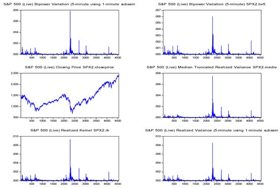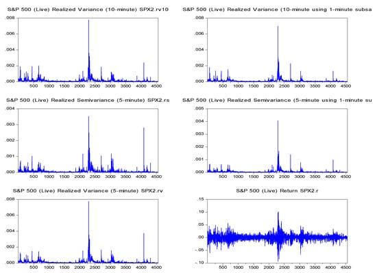
**Figure 1.** S\&P500 plots. Note: This set of figures depict the realized measures on the S\&P500 index (from left to right): The first figure depicts the realized bi-power variation (5-min sub-sampled) estimator, the second figure depicts the realized bi-power variation (5-min) estimator, the third figure depicts the S\&P500 index closing price, the fourth figure depicts the median realized variance (5-min) estimator, the fifth figure depicts the realized Kernel variance estimator (two-scale/Barlett), the sixth figure depicts the realized variance (5-min sub-sampled) estimator, the seventh figure depicts the realized variance (10-min) estimator, the eighth figure depicts the realized variance (10-min sub-sampled) estimator, the ninth figure depicts the realized semi-variance (5-min) estimator, the tenth figure depicts the realized semi-variance (5-min sub-sampled) estimator, the eleventh figure depicts the realized variance (5-min) estimator, and the twelfth figure depicts the return on the S\&P500 index.
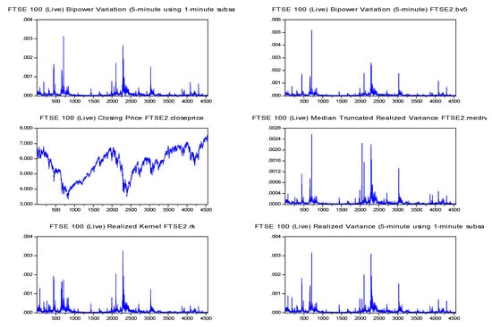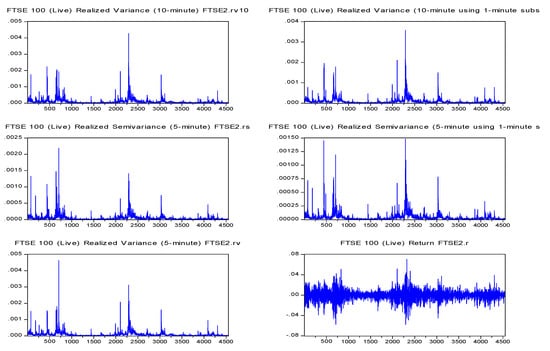
**Figure 2.** FTSE100 plots. Note: This set of figures depict the realized measures on the FTSE100 index (from left to right): The first figure depicts the realized bi-power variation (5-min sub-sampled) estimator, the second figure depicts the realized bi-power variation (5-min) estimator, the third figure depicts the FTSE100 index closing price, the fourth figure depicts the median realized variance (5-min) estimator, the fifth figure depicts the realized Kernel variance estimator (two-scale/Barlett), the sixth figure depicts the realized variance (5-min sub-sampled) estimator, the seventh figure depicts the realized variance (10-min) estimator, the eighth figure depicts the realized variance (10-min sub-sampled) estimator, the ninth figure depicts the realized semi-variance (5-min) estimator, the tenth figure depicts the realized semi-variance (5-min sub-sampled) estimator, the eleventh figure depicts the realized variance (5-min) estimator, and the twelfth figure depicts the return of the FTSE100 index.
### 3\.1. Volatility Feedback Effect
According to [Bekaert and Wu](https://www.mdpi.com/1911-8074/13/6/125#B16-jrfm-13-00125) ([2000](https://www.mdpi.com/1911-8074/13/6/125#B16-jrfm-13-00125)) “If volatility is priced, does an anticipated increase in volatility raise the required return on equity, leading to an immediate stock price decline?”. The empirical evidence related to the relationship between returns and contemporaneous volatility concluded that the volatility feedback effect is mostly statistically insignificant. According to [Bollerslev and Zhou](https://www.mdpi.com/1911-8074/13/6/125#B18-jrfm-13-00125) ([2006](https://www.mdpi.com/1911-8074/13/6/125#B18-jrfm-13-00125)), trade-off between monthly returns and volatilities in a regression framework shows that
𝑏\<0
b
\<
0
. Furthermore, “continuous-time” volatility feedback effect is captured directly by the risk-return trade-off parameter (i.e.,
𝑏\>0
b
\>
0
). The volatility asymmetry effect similar to other markets and time periods is documented in other studies (see [Schwert 1990](https://www.mdpi.com/1911-8074/13/6/125#B56-jrfm-13-00125); [Nelson 1991](https://www.mdpi.com/1911-8074/13/6/125#B52-jrfm-13-00125); [Gallant et al. 1997](https://www.mdpi.com/1911-8074/13/6/125#B30-jrfm-13-00125); [Engle and Ng 1993](https://www.mdpi.com/1911-8074/13/6/125#B28-jrfm-13-00125); [Duffee 1995](https://www.mdpi.com/1911-8074/13/6/125#B27-jrfm-13-00125); [Bekaert and Wu 2000](https://www.mdpi.com/1911-8074/13/6/125#B16-jrfm-13-00125); [Wu 2001](https://www.mdpi.com/1911-8074/13/6/125#B59-jrfm-13-00125), among others).
Against this backdrop, we tested the first hypothesis, namely “volatility feedback effect”. To this end, we estimated the following equation, which presents the returns as a linear function of realized measures:
𝑅𝑡\=𝑏0\+𝑏1𝐵𝑃𝑉𝑡\+𝑏2𝐵𝑃𝑉𝑆𝑆𝑡\+𝑏3𝑀𝑒𝑑𝑅𝑉𝑡\+𝑏4𝑅𝐾𝐵𝑎𝑟𝑙𝑒𝑡𝑡\+𝑏5𝑅𝑆𝑉𝐷𝑡\+𝑏6𝑅𝑆𝑉𝐷,𝑆𝑆𝑡\+𝑏7𝑅𝑉𝑡\+𝑏8𝑅𝑉10,𝑡\+𝑏9𝑅𝑉𝑆𝑆10, 𝑡\+𝑏10𝑅𝑉𝑆𝑆5,𝑡\+𝑢𝑡
R
t
\=
b
0
\+
b
1
B
P
V
t
\+
b
2
B
P
V
t
S
S
\+
b
3
M
e
d
R
V
t
\+
b
4
R
K
t
B
a
r
l
e
t
\+
b
5
R
S
V
t
D
\+
b
6
R
S
V
t
D
,
S
S
\+
b
7
R
V
t
\+
b
8
R
V
10
,
t
\+
b
9
R
V
10
,
t
S
S
\+
b
10
R
V
5
,
t
S
S
\+
u
t
(10)
where
𝑅𝑡
R
t
are the daily returns either for S\&P500 or FTSE100 index,
𝐵𝑃𝑉𝑡
B
P
V
t
is realized bi-power variation (5-min) measure,
𝐵𝑃𝑉𝑆𝑆𝑡
B
P
V
t
S
S
is realized bi-power variation (5-min sub-sampled) measure,
𝑀𝑒𝑑𝑅𝑉𝑡
M
e
d
R
V
t
is median realized variance (5-min),
𝑅𝐾𝐵𝑎𝑟𝑙𝑒𝑡𝑡
R
K
t
B
a
r
l
e
t
is realized Kernel variance (two-scale/Barlett),
𝑅𝑆𝑉𝐷𝑡
R
S
V
t
D
is realized semi-variance (5-min),
𝑅𝑆𝑉𝐷,𝑆𝑆𝑡
R
S
V
t
D
,
S
S
is realized semi-variance (5-min sub-sampled),
𝑅𝑉𝑡
R
V
t
is realized volatility,
𝑅𝑉10,𝑡
R
V
10
,
t
is realized variance (10-min),
𝑅𝑉𝑆𝑆10, 𝑡
R
V
10
,
t
S
S
is realized variance (10-min sub-sampled), and
𝑅𝑉𝑆𝑆5,𝑡
R
V
5
,
t
S
S
is realized variance (5-min sub-sampled). In order to deal with multicollinearity issues that may exist across the realized measure, we employed the variance inflation factor (VIF). We selected 10 out of 13 realized variance estimators in which multicollinearity does not affect our estimation results.
[Table 2](https://www.mdpi.com/1911-8074/13/6/125#table_body_display_jrfm-13-00125-t002) reports the results on the impact of realized measures on returns. Panel A refers to the results from S\&P500, where
𝑀𝑒𝑑𝑅𝑉
M
e
d
R
V
,
𝑅𝑆𝑉𝐷,𝑆𝑆
R
S
V
D
,
S
S
,
𝑅𝑉
R
V
and
𝑅𝑉𝑆𝑆10
R
V
10
S
S
have a statistically significant positive impact on return
𝑅
R
. Additionally,
𝐵𝑃𝑉
B
P
V
,
𝑅𝐾𝐵𝑎𝑟𝑙𝑒𝑡
R
K
B
a
r
l
e
t
,
𝑅𝑆𝑉𝐷
R
S
V
D
,
𝑅𝑉10
R
V
10
and
𝑅𝑉𝑆𝑆5
R
V
5
S
S
have a statistically significant positive impact on return R. Thus, the hypothesis of volatility feedback effect is accepted in the case of S\&P500. Furthermore, Panel B refers to the results of FTSE100. The results show that
𝐵𝑃𝑉𝑆𝑆
B
P
V
S
S
,
𝑀𝑒𝑑𝑅𝑉
M
e
d
R
V
,
𝑅𝑆𝑉𝐷,𝑆𝑆
R
S
V
D
,
S
S
,
𝑅𝑉
R
V
and
𝑅𝑉10
R
V
10
have a statistically significant positive impact on return
𝑅
R
. Further,
𝑅𝑆𝑉𝐷
R
S
V
D
and
𝑅𝑉𝑆𝑆5
R
V
5
S
S
have a statistically significant positive impact on return
𝑅
R
. Thus, the hypothesis of volatility feedback effect is accepted for the case of FTSE100. Our results show that realized measures which affect most the returns are: (i)
𝑅𝑆𝑉𝐷
R
S
V
D
,
𝑅𝑆𝑉𝐷,𝑆𝑆
R
S
V
D
,
S
S
and
𝑅𝑉
R
V
with the marginal impact equal to 0.2244, 0.1341 and 0.0896, respectively, regarding S\&P500, and (ii)
𝑅𝑆𝑉𝐷
R
S
V
D
,
𝑀𝑒𝑑𝑅𝑉
M
e
d
R
V
and
𝑅𝑉𝑆𝑆5
R
V
5
S
S
with the marginal impact equal to 0.0409, 0.0231 and 0.0226, respectively, regarding FTSE100. We found that
𝐵𝑃𝑉
B
P
V
𝑅𝐾𝐵𝑎𝑟𝑙𝑒𝑡
R
K
B
a
r
l
e
t
and
𝑅𝑉𝑆𝑆10
R
V
10
S
S
have impact only on S\&P500 index. Further,
𝐵𝑃𝑉𝑆𝑆
B
P
V
S
S
has impact only on FTSE100 index. The rest of the realized measures have impact on both indices.
**Table 2.** Hypothesis 1 (volatility feedback effect) regression results.

### 3\.2. Leverage Effect Results
According to [Black](https://www.mdpi.com/1911-8074/13/6/125#B17-jrfm-13-00125) ([1976](https://www.mdpi.com/1911-8074/13/6/125#B17-jrfm-13-00125)), “Does a drop in the value of the stock (negative return) increase financial leverage, so that it makes the stock riskier and increases its volatility?”. In the context of empirical assessment related to leverage effect, many volatility models and volatility-return regressions have been used in the existing literature (see, [Bekaert and Wu 2000](https://www.mdpi.com/1911-8074/13/6/125#B16-jrfm-13-00125)). Several studies confirmed that the hypothesis that aggregate stock market volatility asymmetrically reacts to past negative returns (i.e.,
𝑑\<0
d
\<
0
). Leverage effect delineated a negative relation between returns and volatilities; it was first discussed by [Black](https://www.mdpi.com/1911-8074/13/6/125#B17-jrfm-13-00125) ([1976](https://www.mdpi.com/1911-8074/13/6/125#B17-jrfm-13-00125)) and [Christie](https://www.mdpi.com/1911-8074/13/6/125#B22-jrfm-13-00125) ([1982](https://www.mdpi.com/1911-8074/13/6/125#B22-jrfm-13-00125)). Other studies include, [Schwert](https://www.mdpi.com/1911-8074/13/6/125#B56-jrfm-13-00125) ([1990](https://www.mdpi.com/1911-8074/13/6/125#B56-jrfm-13-00125)), [Nelson](https://www.mdpi.com/1911-8074/13/6/125#B52-jrfm-13-00125) ([1991](https://www.mdpi.com/1911-8074/13/6/125#B52-jrfm-13-00125)), [Gallant et al.](https://www.mdpi.com/1911-8074/13/6/125#B29-jrfm-13-00125) ([1992](https://www.mdpi.com/1911-8074/13/6/125#B29-jrfm-13-00125)), [Glosten et al.](https://www.mdpi.com/1911-8074/13/6/125#B40-jrfm-13-00125) ([1993](https://www.mdpi.com/1911-8074/13/6/125#B40-jrfm-13-00125)), [Engle and Ng](https://www.mdpi.com/1911-8074/13/6/125#B28-jrfm-13-00125) ([1993](https://www.mdpi.com/1911-8074/13/6/125#B28-jrfm-13-00125)), [Duffee](https://www.mdpi.com/1911-8074/13/6/125#B27-jrfm-13-00125) ([1995](https://www.mdpi.com/1911-8074/13/6/125#B27-jrfm-13-00125)), [Bekaert and Wu](https://www.mdpi.com/1911-8074/13/6/125#B16-jrfm-13-00125) ([2000](https://www.mdpi.com/1911-8074/13/6/125#B16-jrfm-13-00125)), and [Bollerslev and Zhou](https://www.mdpi.com/1911-8074/13/6/125#B18-jrfm-13-00125) ([2006](https://www.mdpi.com/1911-8074/13/6/125#B18-jrfm-13-00125)).
Against this backdrop, we tested the second hypothesis, namely “leverage effect”. To this end, we estimated realized volatility following [Bekaert and Wu](https://www.mdpi.com/1911-8074/13/6/125#B16-jrfm-13-00125) ([2000](https://www.mdpi.com/1911-8074/13/6/125#B16-jrfm-13-00125)), which presents realized variation as a linear function of returns:
𝑅𝑉𝑡,𝑡\+1\=𝑐\+𝑑𝑅𝑡−1,𝑡\+𝑢𝑡
R
V
t
,
t
\+
1
\=
c
\+
d
R
t
−
1
,
t
\+
u
t
(11)
where
𝑅𝑉
R
V
is the realized volatility and
𝑅
R
is the return.
[Table 3](https://www.mdpi.com/1911-8074/13/6/125#table_body_display_jrfm-13-00125-t003) reports the impact of realized measures on return. Panel A shows that S\&P500 returns have a statistically significant but negative impact on their past returns, with coefficient
𝑑
d
being equal to −1.1040 × 10⁻³ . Moreover, Panel B shows that FTSE100 returns have a statistically significant negative impact on their past returns with coefficient
𝑑
d
being equal to −5.6477 × 10⁻⁴. Hence, in both cases, the hypothesis of leverage effect is accepted.
**Table 3.** Hypothesis 2 (leverage effect) regression results.

## 4\. Practical Implications
In this section, we investigate the out-of-sample forecasting accuracy of our model to forecast returns of S\&P500 and FTSE100. First, we provide the out-of-sample forecasting results, and second, we proceed to a portfolio exercise.
### 4\.1. Out-of-Sample Analysis
We studied the forecasting accuracy of our model and tested Equation (8), which presents the returns as a linear function of realized measures. We provided four different forecast evaluation measures considering (i) mean forecast error (MFE), (ii) mean absolute deviation (MAD), (iii) tracking signal and (iv) the forecast error. We used one step-ahead rolling estimation windows, using a fixed number of the most recent data at each point of time, on the daily equity returns of S\&P500 and FTSE100 indices. To this end, we used a rolling-estimation window of 1000 observations.
As for S\&P500, the mean forecast error was equal to 7.83 × 10⁻³, and the mean absolute deviation was equal to 2.61 × 10⁻⁶ with tracking signal equal to 107.3424. As for FTSE100, the mean forecast error was equal to −6.10 × 10⁻³, and the mean absolute deviation was equal to 2.03 × 10⁻⁶ with tracking signal equal to −222.2500. [Figure 3](https://www.mdpi.com/1911-8074/13/6/125#fig_body_display_jrfm-13-00125-f003) depicts the forecast error both for of S\&P500 and FTSE100 index.
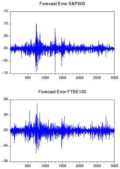
**Figure 3.** Forecast errors plots. Note: This set of figures depicts the one-step-ahead forecast error of the expected returns in S\&P500 and FTSE100 indices used in this study obtained from a rolling-estimation window of 1000 observations.
We further computed the forecasting strength of our model (Equation (8)) and removed the periods of high volatility. In particular, we estimated Equation (8) excluding high and low volatility regimes. [Figure 4](https://www.mdpi.com/1911-8074/13/6/125#fig_body_display_jrfm-13-00125-f004) depicts various volatility regimes obtained from S\&P500 (Panel A) and FTSE100 (Panel B). In both panels, green and red colors depict various periods of high and low volatility, respectively. Further, [Figure 5](https://www.mdpi.com/1911-8074/13/6/125#fig_body_display_jrfm-13-00125-f005) depicts two sets of figures (i) the volatility regimes in returns (upper figure) and (ii) the probability of the high and low volatility regimes (bottom figure) of S\&P500 and FTSE100 indices. Panel A refers to S\&P500 index sample. Panel B refers to FTSE100 index sample.

**Figure 4.** Volatility regimes. Note: This set figures depicts the volatility regimes in returns and equity prices of S\&P500 and FTSE100 indices; the green color refers to high volatility regimes while the red color refers to low volatility regimes. Panel A refers to S\&P500 index sample. Panel B refers to FTSE100 index sample.
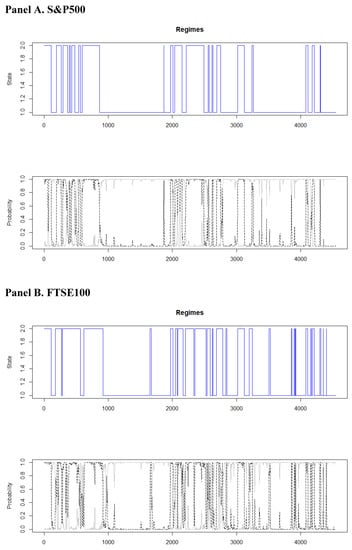
**Figure 5.** Defined volatility regimes. Note: This set figures depicts the volatility regimes in returns (upper figure) and the probability of the high and low volatility regimes (bottom figure) of S\&P500 and FTSE100 indices. On the bottom figure, the grey color refers to high volatility regimes while the black color refers to low volatility regimes. Panel A refers to S\&P500 index sample. Panel B refers to FTSE100 index sample.
[Table 4](https://www.mdpi.com/1911-8074/13/6/125#table_body_display_jrfm-13-00125-t004) presents R adjusted (R adj.) estimation results of our model (Equation (8)) in low and high volatility regimes. In particular, we picked 10 regimes (obtained by [Figure 4](https://www.mdpi.com/1911-8074/13/6/125#fig_body_display_jrfm-13-00125-f004) and [Figure 5](https://www.mdpi.com/1911-8074/13/6/125#fig_body_display_jrfm-13-00125-f005)), five lower volatility regimes and five higher volatility regimes (we selected the regimes with the higher number of observations). R adjusted (R adj.) of Equation (8) for low and high volatility regimes are reported in [Table 4](https://www.mdpi.com/1911-8074/13/6/125#table_body_display_jrfm-13-00125-t004), where again Panel A refers to S\&P500 index and Panel B refers to FTSE100 index. As for S\&P500 (Panel A) in low volatility regimes, we found that R adj had max equal to
0\.8274
0\.8274
and min equal to
0\.7377
0\.7377
, while in high volatility regimes the R adj had max equal to
0\.8809
0\.8809
and min equal to
0\.7452
0\.7452
. As for FTSE100 (Panel B) in low volatility regimes, we found that R adj had max equal to
0\.7934
0\.7934
and min equal to
0\.6416
0\.6416
, while in high volatility regimes the R adj had max equal to
0\.8731
0\.8731
and min equal to
0\.7697
0\.7697
. Such evidence indicates that the predictability of our model is qualitatively similar between periods of low and high levels of volatility.
**Table 4.** Estimation results in low and high volatility regimes.

### 4\.2. Portfolio Implications
We now proceed to a portfolio exercise to provide practical implications of the results obtained from our study. We took the point of view of investors in equity markets and we constructed two-asset portfolios: the first included the actual returns of the S\&P500 and FTSE100 indices, while the second included the expected returns of the S\&P500 and FTSE100 indices obtained from Equation (8). Consequently, we analyzed the optimal portfolio weights using actual and expected returns. We employed mean-variance portfolios based on [Markowitz](https://www.mdpi.com/1911-8074/13/6/125#B49-jrfm-13-00125) ([1952](https://www.mdpi.com/1911-8074/13/6/125#B49-jrfm-13-00125)) to compute the optimal weighs (see [also Gkillas and Longin 2019](https://www.mdpi.com/1911-8074/13/6/125#B34-jrfm-13-00125)). Considering the portfolio with the actual returns, the weights of FTSE100 and S\&P500 asset were equal to
0\.7172
0\.7172
and
0\.2825
0\.2825
, respectively, while in the portfolio with the expected returns, the weights of FTSE100 and S\&P500 asset were equal to
0\.7055
0\.7055
and
0\.2939
0\.2939
, respectively. Again, such evidence indicates that our estimates are reasonable accurate.
## 5\. Summary and Conclusions
In this study, we investigated the impact of the realized measures on returns and vice versa, considering S\&P500 and FTSE100 indices for the period spans from January 2000 to June 2017. Specifically, we empirically examined two research questions as follows: “If volatility is priced, does an anticipated increase in volatility raise the required return on equity on S\&P500 and FTSE100 index?” and “Does a drop in the value of the stock (negative return) increase financial leverage, so that it makes the stock riskier and increases its volatility on S\&P500 and FTSE100 index?”. We considered 10 realized measures from the Oxford-Man Institute of Quantitative Finance database to examine two hypotheses associated with the financial modelling and decision-making: (i) the volatility feedback effect as the relationship between the contemporaneous returns and the market-based volatility and (ii) the leverage effect as the relationship between lagged returns and the current market-based volatility.
As for the first research question, we found a positive relationship between the volatility and returns. The results were as follows for volatility feedback effect: for S\&P500, most of the realized measures had a significant positive effect on daily returns
𝐵𝑃𝑉
B
P
V
,
𝑀𝑒𝑑𝑅𝑉
M
e
d
R
V
,
𝑅𝐾𝐵𝑎𝑟𝑙𝑒𝑡
R
K
B
a
r
l
e
t
,
𝑅𝑆𝑉𝐷
R
S
V
D
,
𝑅𝑆𝑉𝐷,𝑆𝑆
R
S
V
D
,
S
S
,
𝑅𝑉
R
V
,
𝑅𝑉10
R
V
10
,
𝑅𝑉𝑆𝑆10
R
V
10
S
S
and
𝑅𝑉𝑆𝑆5
R
V
5
S
S
. For FTSE100, most of the realized measures had a significant positive effect on daily returns:
𝐵𝑃𝑉𝑆𝑆
B
P
V
S
S
,
𝑀𝑒𝑑𝑅𝑉
M
e
d
R
V
,
𝑅𝑆𝑉𝐷
R
S
V
D
,
𝑅𝑆𝑉𝐷,𝑆𝑆
R
S
V
D
,
S
S
,
𝑅𝑉
R
V
,
𝑅𝑉10
R
V
10
and
𝑅𝑉𝑆𝑆5
R
V
5
S
S
. Both realized
𝑅𝐾𝐵𝑎𝑟𝑙𝑒𝑡
R
K
B
a
r
l
e
t
and
𝑅𝑉𝑆𝑆10
R
V
10
S
S
had no effect on returns for FTSE100. An increase on “continuous-time” volatility raised the required return on both equity markets capturing the risk-return trade-off effect, which is consistent to [Bollerslev and Zhou](https://www.mdpi.com/1911-8074/13/6/125#B18-jrfm-13-00125) ([2006](https://www.mdpi.com/1911-8074/13/6/125#B18-jrfm-13-00125)). Furthermore, as for the second hypothesis, we found a negative relationship between the lag-returns and the volatility. With regard to the leverage effect hypothesis, both S\&P500 and FTSE100 indices show that returns negatively affect realized volatility, which indicates that downside returns make the stocks riskier and increase their volatility. We confirmed the stylized fact of leverage effect, in which returns are negatively correlated with realized volatility ([Corsi et al. 2012](https://www.mdpi.com/1911-8074/13/6/125#B23-jrfm-13-00125)). Such evidence for S\&P500 and FTSE100 indices is consistent with the existing literature. Overall, we conclude that realized measures change and affect differently the daily returns of financial indices.
Future research should examine forecasting accuracy, that is, if implied volatilities provide unbiased and informationally efficient forecasts of the corresponding future realized volatilities.
## Author Contributions
Authors have equal contributions. All authors have read and agreed to the published version of the manuscript.
## Funding
This research received no external funding.
## Acknowledgments
We thank two anonymous reviewers and the participants of the “7th International Conference on Multidimensional Finance, Insurance and Investment” (Chania, Greece, May 2018) for their valuable comments.
## Conflicts of Interest
The authors declare no conflict of interest.
## References
1. Alghalith, Moawia, Christos Floros, and Konstantinos Gkillas. 2020. Estimating stochastic volatility under the assumption of stochastic volatility of volatility. Risks 8: 35. \[[Google Scholar](https://scholar.google.com/scholar_lookup?title=Estimating+stochastic+volatility+under+the+assumption+of+stochastic+volatility+of+volatility&author=Alghalith,+Moawia&author=Christos+Floros&author=and+Konstantinos+Gkillas&publication_year=2020&journal=Risks&volume=8&pages=35&doi=10.3390/risks8020035)\] \[[CrossRef](https://doi.org/10.3390/risks8020035)\]
2. Andersen, Torben G., and Tim Bollerslev. 1998. Answering the Skeptics: Yes, Standard Volatility Models do Provide Accurate Forecasts. International Economic Review 39: 885. \[[Google Scholar](https://scholar.google.com/scholar_lookup?title=Answering+the+Skeptics:+Yes,+Standard+Volatility+Models+do+Provide+Accurate+Forecasts&author=Andersen,+Torben+G.&author=and+Tim+Bollerslev&publication_year=1998&journal=International+Economic+Review&volume=39&pages=885&doi=10.2307/2527343)\] \[[CrossRef](https://doi.org/10.2307/2527343)\]
3. Andersen, Torben G., Tim Bollerslev, Francis X. Diebold, and Heiko Ebens. 2001a. The distribution of realized stock return volatility. Journal of Financial Economics 61: 43–76. \[[Google Scholar](https://scholar.google.com/scholar_lookup?title=The+distribution+of+realized+stock+return+volatility&author=Andersen,+Torben+G.&author=Tim+Bollerslev&author=Francis+X.+Diebold&author=and+Heiko+Ebens&publication_year=2001a&journal=Journal+of+Financial+Economics&volume=61&pages=43%E2%80%9376&doi=10.1016/S0304-405X\(01\)00055-1)\] \[[CrossRef](https://doi.org/10.1016/S0304-405X\(01\)00055-1)\]
4. Andersen, Torben G., Tim Bollerslev, Francis X. Diebold, and Paul Labys. 2001b. The Distribution of Realized Exchange Rate Volatility. Journal of the American Statistical Association 96: 42–55. \[[Google Scholar](https://scholar.google.com/scholar_lookup?title=The+Distribution+of+Realized+Exchange+Rate+Volatility&author=Andersen,+Torben+G.&author=Tim+Bollerslev&author=Francis+X.+Diebold&author=and+Paul+Labys&publication_year=2001b&journal=Journal+of+the+American+Statistical+Association&volume=96&pages=42%E2%80%9355&doi=10.1198/016214501750332965)\] \[[CrossRef](https://doi.org/10.1198/016214501750332965)\]
5. Andersen, Torben G., Tim Bollerslev, Francis X. Diebold, and Clara Vega. 2007. Real-time price discovery in global stock, bond and foreign exchange markets. Journal of International Economics 73: 251–77. \[[Google Scholar](https://scholar.google.com/scholar_lookup?title=Real-time+price+discovery+in+global+stock,+bond+and+foreign+exchange+markets&author=Andersen,+Torben+G.&author=Tim+Bollerslev&author=Francis+X.+Diebold&author=and+Clara+Vega&publication_year=2007&journal=Journal+of+International+Economics&volume=73&pages=251%E2%80%9377&doi=10.1016/j.jinteco.2007.02.004)\] \[[CrossRef](https://doi.org/10.1016/j.jinteco.2007.02.004)\]
6. Andersen, Torben G., Tim Bollerslev, and Nour Meddahi. 2011. Realized volatility forecasting and market microstructure noise. Journal of Econometrics 160: 220–234. \[[Google Scholar](https://scholar.google.com/scholar_lookup?title=Realized+volatility+forecasting+and+market+microstructure+noise&author=Andersen,+Torben+G.&author=Tim+Bollerslev&author=and+Nour+Meddahi&publication_year=2011&journal=Journal+of+Econometrics&volume=160&pages=220%E2%80%93234&doi=10.1016/j.jeconom.2010.03.032)\] \[[CrossRef](https://doi.org/10.1016/j.jeconom.2010.03.032)\]
7. Andersen, Torben G., Dobrislav Dobrev, and Ernst Schaumburg. 2012. Jump-robust volatility estimation using nearest neighbor truncation. Journal of Econometrics 169: 75–93. \[[Google Scholar](https://scholar.google.com/scholar_lookup?title=Jump-robust+volatility+estimation+using+nearest+neighbor+truncation&author=Andersen,+Torben+G.&author=Dobrislav+Dobrev&author=and+Ernst+Schaumburg&publication_year=2012&journal=Journal+of+Econometrics&volume=169&pages=75%E2%80%9393&doi=10.1016/j.jeconom.2012.01.011)\] \[[CrossRef](https://doi.org/10.1016/j.jeconom.2012.01.011)\]
8. Ang, Andrew, Robert J. Hodrick, Yuhang Xing, and Xiaoyan Zhang. 2006. The Cross-Section of Volatility and Expected Returns. The Journal of Finance 61: 259–99. \[[Google Scholar](https://scholar.google.com/scholar_lookup?title=The+Cross-Section+of+Volatility+and+Expected+Returns&author=Ang,+Andrew&author=Robert+J.+Hodrick&author=Yuhang+Xing&author=and+Xiaoyan+Zhang&publication_year=2006&journal=The+Journal+of+Finance&volume=61&pages=259%E2%80%9399&doi=10.1111/j.1540-6261.2006.00836.x)\] \[[CrossRef](https://doi.org/10.1111/j.1540-6261.2006.00836.x)\]
9. Bali, Turan G., and Panayiotis Theodossiou. 2007. A Conditional-SGT-VaR Approach with Alternative GARCH Models. Annals of Operations Research 151: 241–67. \[[Google Scholar](https://scholar.google.com/scholar_lookup?title=A+Conditional-SGT-VaR+Approach+with+Alternative+GARCH+Models&author=Bali,+Turan+G.&author=and+Panayiotis+Theodossiou&publication_year=2007&journal=Annals+of+Operations+Research&volume=151&pages=241%E2%80%9367&doi=10.1007/s10479-006-0118-4)\] \[[CrossRef](https://doi.org/10.1007/s10479-006-0118-4)\]
10. Barndorff-Nielsen, Ole E., and Neil Shephard. 2002. Econometric analysis of realized volatility and its use in estimating stochastic volatility models. Journal of the Royal Statistical Society: Series B (Statistical Methodology) 64: 253–80. \[[Google Scholar](https://scholar.google.com/scholar_lookup?title=Econometric+analysis+of+realized+volatility+and+its+use+in+estimating+stochastic+volatility+models&author=Barndorff-Nielsen,+Ole+E.&author=and+Neil+Shephard&publication_year=2002&journal=Journal+of+the+Royal+Statistical+Society:+Series+B+\(Statistical+Methodology\)&volume=64&pages=253%E2%80%9380&doi=10.1111/1467-9868.00336)\] \[[CrossRef](https://doi.org/10.1111/1467-9868.00336)\]
11. Barndorff-Nielsen, Ole E., and Neil Shephard. 2004. Power and Bipower Variation with Stochastic Volatility and Jumps. Journal of Financial Econometrics 2: 1–37. \[[Google Scholar](https://scholar.google.com/scholar_lookup?title=Power+and+Bipower+Variation+with+Stochastic+Volatility+and+Jumps&author=Barndorff-Nielsen,+Ole+E.&author=and+Neil+Shephard&publication_year=2004&journal=Journal+of+Financial+Econometrics&volume=2&pages=1%E2%80%9337&doi=10.1093/jjfinec/nbh001)\] \[[CrossRef](https://doi.org/10.1093/jjfinec/nbh001)\]
12. Barndorff-Nielsen, Ole E., and Neil Shephard. 2006. Econometrics of Testing for Jumps in Financial Economics Using Bipower Variation. Journal of Financial Econometrics 4: 1–30. \[[Google Scholar](https://scholar.google.com/scholar_lookup?title=Econometrics+of+Testing+for+Jumps+in+Financial+Economics+Using+Bipower+Variation&author=Barndorff-Nielsen,+Ole+E.&author=and+Neil+Shephard&publication_year=2006&journal=Journal+of+Financial+Econometrics&volume=4&pages=1%E2%80%9330&doi=10.1093/jjfinec/nbi022)\] \[[CrossRef](https://doi.org/10.1093/jjfinec/nbi022)\]
13. Barndorff-Nielsen, Ole E., Peter Reinhard Hansen, Asger Lunde, and Neil Shephard. 2008. Designing Realized Kernels to Measure the ex post Variation of Equity Prices in the Presence of Noise. Econometrica 76: 1481–536. \[[Google Scholar](https://scholar.google.com/scholar_lookup?title=Designing+Realized+Kernels+to+Measure+the+ex+post+Variation+of+Equity+Prices+in+the+Presence+of+Noise&author=Barndorff-Nielsen,+Ole+E.&author=Peter+Reinhard+Hansen&author=Asger+Lunde&author=and+Neil+Shephard&publication_year=2008&journal=Econometrica&volume=76&pages=1481%E2%80%93536&doi=10.3982/ECTA6495)\] \[[CrossRef](https://doi.org/10.3982/ECTA6495)\]
14. Barndorff-Nielsen, Ole E., Peter Reinhard Hansen, Asger Lunde, and Neil Shephard. 2009. Realized kernels in practice: Trades and quotes. Econometrics Journal 12: C1–C32. \[[Google Scholar](https://scholar.google.com/scholar_lookup?title=Realized+kernels+in+practice:+Trades+and+quotes&author=Barndorff-Nielsen,+Ole+E.&author=Peter+Reinhard+Hansen&author=Asger+Lunde&author=and+Neil+Shephard&publication_year=2009&journal=Econometrics+Journal&volume=12&pages=C1%E2%80%93C32&doi=10.1111/j.1368-423X.2008.00275.x)\] \[[CrossRef](https://doi.org/10.1111/j.1368-423X.2008.00275.x)\]
15. Barndorff-Nielsen, Ole E., Silja Kinnebrock, and Neil Shephard. 2010. Measuring Downside Risk-Realised Semivariance. In Volatility and Time Series Econometrics: Essays in Honor of Robert F. Engle. Edited by Tim Bollerslev, Jerrrey Russell and Mark Watson. New York: Oxford University Press, pp. 117–37. \[[Google Scholar](https://scholar.google.com/scholar_lookup?title=Measuring+Downside+Risk-Realised+Semivariance&author=Barndorff-Nielsen,+Ole+E.&author=Silja+Kinnebrock&author=and+Neil+Shephard&publication_year=2010&pages=117%E2%80%9337)\]
16. Bekaert, Geert, and Guojun Wu. 2000. Asymmetric Volatility and Risk in Equity Markets. Review of Financial Studies 13: 1–42. \[[Google Scholar](https://scholar.google.com/scholar_lookup?title=Asymmetric+Volatility+and+Risk+in+Equity+Markets&author=Bekaert,+Geert&author=and+Guojun+Wu&publication_year=2000&journal=Review+of+Financial+Studies&volume=13&pages=1%E2%80%9342&doi=10.1093/rfs/13.1.1)\] \[[CrossRef](https://doi.org/10.1093/rfs/13.1.1)\]
17. Black, Fischer. 1976. Studies of Stock Price Volatility Changes. In Proceedings of the Business and Economics Section. Washington: American Statistical Association, pp. 177–81. \[[Google Scholar](https://scholar.google.com/scholar_lookup?title=Studies+of+Stock+Price+Volatility+Changes&author=Black,+Fischer&publication_year=1976&pages=177%E2%80%9381)\]
18. Bollerslev, Tim, and Hao Zhou. 2006. Volatility puzzles: A simple framework for gauging return-volatility regressions. Journal of Econometrics 131: 123–50. \[[Google Scholar](https://scholar.google.com/scholar_lookup?title=Volatility+puzzles:+A+simple+framework+for+gauging+return-volatility+regressions&author=Bollerslev,+Tim&author=and+Hao+Zhou&publication_year=2006&journal=Journal+of+Econometrics&volume=131&pages=123%E2%80%9350&doi=10.1016/j.jeconom.2005.01.006)\] \[[CrossRef](https://doi.org/10.1016/j.jeconom.2005.01.006)\]
19. Bollerslev, Tim, Sophia Zhengzi Li, and Bingzhi Zhao. 2019. Good Volatility, Bad Volatility, and the Cross Section of Stock Returns. Journal of Financial and Quantitative Analysis 55: 751–81. \[[Google Scholar](https://scholar.google.com/scholar_lookup?title=Good+Volatility,+Bad+Volatility,+and+the+Cross+Section+of+Stock+Returns&author=Bollerslev,+Tim&author=Sophia+Zhengzi+Li&author=and+Bingzhi+Zhao&publication_year=2019&journal=Journal+of+Financial+and+Quantitative+Analysis&volume=55&pages=751%E2%80%9381&doi=10.1017/S0022109019000097)\] \[[CrossRef](https://doi.org/10.1017/S0022109019000097)\]
20. Campbell, John Y., and Ludger Hentschel. 1992. No News Is Good News: An Asymmetric Model of Changing Volatility in Stock Returns. Journal of Financial Economics 31: 281–318. Available online: <https://www.sciencedirect.com/science/article/pii/0304405X9290037X> (accessed on 22 April 2002). \[[CrossRef](https://doi.org/10.1016/0304-405X\(92\)90037-X)\]
21. Carr, Peter, and Liuren Wu. 2017. Leverage Effect, Volatility Feedback, and Self-Exciting Market Disruptions. Journal of Financial and Quantitative Analysis 52: 2119–56. \[[Google Scholar](https://scholar.google.com/scholar_lookup?title=Leverage+Effect,+Volatility+Feedback,+and+Self-Exciting+Market+Disruptions&author=Carr,+Peter&author=and+Liuren+Wu&publication_year=2017&journal=Journal+of+Financial+and+Quantitative+Analysis&volume=52&pages=2119%E2%80%9356&doi=10.1017/S0022109017000564)\] \[[CrossRef](https://doi.org/10.1017/S0022109017000564)\]
22. Christie, Andrew A. 1982. The Stochastic Behavior of Common Stock Variances: Value, Leverage and Interest Rate Effects. Journal of Financial Economics 10: 407–32. Available online: <https://www.sciencedirect.com/science/article/pii/0304405X82900186> (accessed on 15 April 2002).
23. Corsi, Fulvio, Francesco Audrino, and Roberto Renó. 2012. HAR Modeling for Realized Volatility Forecasting. In Handbook of Volatility Models and their Applications. Edited by Luc Bauwens, Christian M. Hafner and Sebastien Laurent. New York: Wiley & Sons Ltd. \[[Google Scholar](https://scholar.google.com/scholar_lookup?title=HAR+Modeling+for+Realized+Volatility+Forecasting&author=Corsi,+Fulvio&author=Francesco+Audrino&author=and+Roberto+Ren%C3%B3&publication_year=2012)\]
24. Degiannakis, Stavros, and Christos Floros. 2015. Modelling and Forecasting High Frequency Financial Data. Hampshire: Palgrave-MacMillan Ltd. \[[Google Scholar](https://scholar.google.com/scholar_lookup?title=Modelling+and+Forecasting+High+Frequency+Financial+Data&author=Degiannakis,+Stavros&author=and+Christos+Floros&publication_year=2015)\]
25. Degiannakis, Stavros, and Christos Floros. 2016. Intra-Day Realized Volatility for European and USA Stock Indices. Global Finance Journal 29: 24–41. \[[Google Scholar](https://scholar.google.com/scholar_lookup?title=Intra-Day+Realized+Volatility+for+European+and+USA+Stock+Indices&author=Degiannakis,+Stavros&author=and+Christos+Floros&publication_year=2016&journal=Global+Finance+Journal&volume=29&pages=24%E2%80%9341&doi=10.1016/j.gfj.2015.05.002)\] \[[CrossRef](https://doi.org/10.1016/j.gfj.2015.05.002)\]
26. Demirer, Riza, Konstantinos Gkillas, Rangan Gupta, and Christian Pierdzioch. 2019. Time-varying risk aversion and realized gold volatility. North American Journal of Economics and Finance 50: 101048. \[[Google Scholar](https://scholar.google.com/scholar_lookup?title=Time-varying+risk+aversion+and+realized+gold+volatility&author=Demirer,+Riza&author=Konstantinos+Gkillas&author=Rangan+Gupta&author=and+Christian+Pierdzioch&publication_year=2019&journal=North+American+Journal+of+Economics+and+Finance&volume=50&pages=101048&doi=10.1016/j.najef.2019.101048)\] \[[CrossRef](https://doi.org/10.1016/j.najef.2019.101048)\]
27. Duffee, Gregory R. 1995. Stock Returns and Volatility a Firm-Level Analysis. Journal of Financial Economics 37: 399–420. Available online: <https://www.sciencedirect.com/science/article/pii/0304405X94008017> (accessed on 7 March 2000).
28. Engle, Robert F., and Victor K. Ng. 1993. Measuring and Testing the Impact of News on Volatility. The Journal of Finance 48: 1749–78. \[[Google Scholar](https://scholar.google.com/scholar_lookup?title=Measuring+and+Testing+the+Impact+of+News+on+Volatility&author=Engle,+Robert+F.&author=and+Victor+K.+Ng&publication_year=1993&journal=The+Journal+of+Finance&volume=48&pages=1749%E2%80%9378&doi=10.1111/j.1540-6261.1993.tb05127.x)\] \[[CrossRef](https://doi.org/10.1111/j.1540-6261.1993.tb05127.x)\]
29. Gallant, A. Ronald, Peter E. Rossi, and George Tauchen. 1992. Stock Prices and Volume. Review of Financial Studies 5: 199–242. \[[Google Scholar](https://scholar.google.com/scholar_lookup?title=Stock+Prices+and+Volume&author=Gallant,+A.+Ronald&author=Peter+E.+Rossi&author=and+George+Tauchen&publication_year=1992&journal=Review+of+Financial+Studies&volume=5&pages=199%E2%80%93242&doi=10.1093/rfs/5.2.199)\] \[[CrossRef](https://doi.org/10.1093/rfs/5.2.199)\]
30. Gallant, A. Ronald, David Hsieh, and George Tauchen. 1997. Estimation of stochastic volatility models with diagnostics. Journal of Econometrics 81: 159–92. \[[Google Scholar](https://scholar.google.com/scholar_lookup?title=Estimation+of+stochastic+volatility+models+with+diagnostics&author=Gallant,+A.+Ronald&author=David+Hsieh&author=and+George+Tauchen&publication_year=1997&journal=Journal+of+Econometrics&volume=81&pages=159%E2%80%9392&doi=10.1016/S0304-4076\(97\)00039-0)\] \[[CrossRef](https://doi.org/10.1016/S0304-4076\(97\)00039-0)\]
31. Ghysels, Eric, and Arthur Sinko. 2011. Volatility forecasting and microstructure noise. Journal of Econometrics 160: 257–71. \[[Google Scholar](https://scholar.google.com/scholar_lookup?title=Volatility+forecasting+and+microstructure+noise&author=Ghysels,+Eric&author=and+Arthur+Sinko&publication_year=2011&journal=Journal+of+Econometrics&volume=160&pages=257%E2%80%9371&doi=10.1016/j.jeconom.2010.03.035)\] \[[CrossRef](https://doi.org/10.1016/j.jeconom.2010.03.035)\]
32. Giot, Pierre, Sébastien Laurent, and Mikael Petitjean. 2010. Trading activity realized volatility and jumps. Journal of Empirical Finance 17: 168–75. \[[Google Scholar](https://scholar.google.com/scholar_lookup?title=Trading+activity+realized+volatility+and+jumps&author=Giot,+Pierre&author=S%C3%A9bastien+Laurent&author=and+Mikael+Petitjean&publication_year=2010&journal=Journal+of+Empirical+Finance&volume=17&pages=168%E2%80%9375&doi=10.1016/j.jempfin.2009.07.001)\] \[[CrossRef](https://doi.org/10.1016/j.jempfin.2009.07.001)\]
33. Gkillas (Gillas), Konstantinos, Dimitrios I. Vortelinos, and Shrabani Saha. 2018. The properties of realized volatility and realized correlation: Evidence from the Indian stock market. Physica A: Statistical Mechanics and Its Applications 492: 343–59. \[[Google Scholar](https://scholar.google.com/scholar_lookup?title=The+properties+of+realized+volatility+and+realized+correlation:+Evidence+from+the+Indian+stock+market&author=Gkillas+\(Gillas\),+Konstantinos&author=Dimitrios+I.+Vortelinos&author=and+Shrabani+Saha&publication_year=2018&journal=Physica+A:+Statistical+Mechanics+and+Its+Applications&volume=492&pages=343%E2%80%9359&doi=10.1016/j.physa.2017.10.007)\] \[[CrossRef](https://doi.org/10.1016/j.physa.2017.10.007)\]
34. Gkillas, Konstantinos, and François Longin. 2019. Is Bitcoin the New Digital Gold? Evidence from Extreme Price Movements in Financial Markets. Available online: <http://dx.doi.org/10.2139/ssrn.3245571> (accessed on 26 September 2018).
35. Gkillas, Konstantinos, Dimitrios Vortelinos, Christos Floros, Alexandros Garefalakis, and Nikolaos Sariannidis. 2019a. Greek Sovereign Crisis and European Exchange Rates: Effects of News Releases and Their Providers. Annals of Operations Research, 1–22. Available online: <http://link.springer.com/10.1007/s10479-019-03199-x> (accessed on 9 April 2019). \[[CrossRef](https://doi.org/10.1007/s10479-019-03199-x)\]
36. Gkillas, Konstantinos, Rangan Gupta, and Christian Pierdzioch. 2019b. Forecasting realized gold volatility: Is there a role of geopolitical risks? Finance Research Letters. \[[Google Scholar](https://scholar.google.com/scholar_lookup?title=Forecasting+realized+gold+volatility:+Is+there+a+role+of+geopolitical+risks?&author=Gkillas,+Konstantinos&author=Rangan+Gupta&author=and+Christian+Pierdzioch&publication_year=2019b&journal=Finance+Research+Letters&doi=10.1016/j.frl.2019.08.028)\] \[[CrossRef](https://doi.org/10.1016/j.frl.2019.08.028)\]
37. Gkillas, Konstantinos, Rangan Gupta, Chi Keung Marco Lau, and Muhammad Tahir Suleman. 2020a. Jumps beyond the realms of cricket: India’s performance in One Day Internationals and stock market movements. Journal of Applied Statistics 47: 1109–27. \[[Google Scholar](https://scholar.google.com/scholar_lookup?title=Jumps+beyond+the+realms+of+cricket:+India%E2%80%99s+performance+in+One+Day+Internationals+and+stock+market+movements&author=Gkillas,+Konstantinos&author=Rangan+Gupta&author=Chi+Keung+Marco+Lau&author=and+Muhammad+Tahir+Suleman&publication_year=2020a&journal=Journal+of+Applied+Statistics&volume=47&pages=1109%E2%80%9327&doi=10.1080/02664763.2019.1663157)\] \[[CrossRef](https://doi.org/10.1080/02664763.2019.1663157)\]
38. Gkillas, Konstantinos, Rangan Gupta, and Christian Pierdzioch. 2020b. Forecasting realized oil-price volatility: The role of financial stress and asymmetric loss. Journal of International Money and Finance 104: 102137. \[[Google Scholar](https://scholar.google.com/scholar_lookup?title=Forecasting+realized+oil-price+volatility:+The+role+of+financial+stress+and+asymmetric+loss&author=Gkillas,+Konstantinos&author=Rangan+Gupta&author=and+Christian+Pierdzioch&publication_year=2020b&journal=Journal+of+International+Money+and+Finance&volume=104&pages=102137&doi=10.1016/j.jimonfin.2020.102137)\] \[[CrossRef](https://doi.org/10.1016/j.jimonfin.2020.102137)\]
39. Gkillas, Konstantinos, Rangan Gupta, and Mark E. Wohar. 2020c. Oil shocks and volatility jumps. Review of Quantitative Finance and Accounting 54: 247–72. \[[Google Scholar](https://scholar.google.com/scholar_lookup?title=Oil+shocks+and+volatility+jumps&author=Gkillas,+Konstantinos&author=Rangan+Gupta&author=and+Mark+E.+Wohar&publication_year=2020c&journal=Review+of+Quantitative+Finance+and+Accounting&volume=54&pages=247%E2%80%9372&doi=10.1007/s11156-018-00788-y)\] \[[CrossRef](https://doi.org/10.1007/s11156-018-00788-y)\]
40. Glosten, Lawrence R., Ravi Jagannathan, and David E. Runkle. 1993. On the Relation between the Expected Value and the Volatility of the Nominal Excess Return on Stocks. The Journal of Finance 48: 1779–801. \[[Google Scholar](https://scholar.google.com/scholar_lookup?title=On+the+Relation+between+the+Expected+Value+and+the+Volatility+of+the+Nominal+Excess+Return+on+Stocks&author=Glosten,+Lawrence+R.&author=Ravi+Jagannathan&author=and+David+E.+Runkle&publication_year=1993&journal=The+Journal+of+Finance&volume=48&pages=1779%E2%80%93801&doi=10.1111/j.1540-6261.1993.tb05128.x)\] \[[CrossRef](https://doi.org/10.1111/j.1540-6261.1993.tb05128.x)\]
41. Hansen, Peter Reinhard, and Guillaume Horel. 2009. Quadratic Variation by Markov Chains. SSRN Electronic Journal. \[[Google Scholar](https://scholar.google.com/scholar_lookup?title=Quadratic+Variation+by+Markov+Chains&author=Hansen,+Peter+Reinhard&author=and+Guillaume+Horel&publication_year=2009&journal=SSRN+Electronic+Journal&doi=10.2139/ssrn.1367519)\] \[[CrossRef](https://doi.org/10.2139/ssrn.1367519)\]
42. Hansen, Peter Reinhard, and Zhuo Huang. 2016. Exponential GARCH Modeling with Realized Measures of Volatility. Journal of Business & Economic Statistics 34: 269–87. \[[Google Scholar](https://scholar.google.com/scholar_lookup?title=Exponential+GARCH+Modeling+with+Realized+Measures+of+Volatility&author=Hansen,+Peter+Reinhard&author=and+Zhuo+Huang&publication_year=2016&journal=Journal+of+Business+&+Economic+Statistics&volume=34&pages=269%E2%80%9387&doi=10.1080/07350015.2015.1038543)\] \[[CrossRef](https://doi.org/10.1080/07350015.2015.1038543)\]
43. Hansen, Peter R., and Asger Lunde. 2006. Realized Variance and Market Microstructure Noise. Journal of Business & Economic Statistics 24: 127–61. \[[Google Scholar](https://scholar.google.com/scholar_lookup?title=Realized+Variance+and+Market+Microstructure+Noise&author=Hansen,+Peter+R.&author=and+Asger+Lunde&publication_year=2006&journal=Journal+of+Business+&+Economic+Statistics&volume=24&pages=127%E2%80%9361&doi=10.1198/073500106000000071)\] \[[CrossRef](https://doi.org/10.1198/073500106000000071)\]
44. Jacod, Jean. 2007. Statistics and High Frequency Data: SEMSTAT Seminar. Technical Report, Université de Paris-6. \[1513\]. Paris: Université de Paris. \[[Google Scholar](https://scholar.google.com/scholar_lookup?title=Statistics+and+High+Frequency+Data:+SEMSTAT+Seminar&author=Jacod,+Jean&publication_year=2007)\]
45. Kiliç, Deniz Kenan, and Ömür Ugur. 2018. Multiresolution Analysis of S\&P500 Time Series. Annals of Operations Research 260: 197–216. \[[Google Scholar](https://scholar.google.com/scholar_lookup?title=Multiresolution+Analysis+of+S%2526P500+Time+Series&author=Kili%C3%A7,+Deniz+Kenan&author=and+%C3%96m%C3%BCr+Ugur&publication_year=2018&journal=Annals+of+Operations+Research&volume=260&pages=197%E2%80%93216&doi=10.1007/s10479-016-2215-3)\] \[[CrossRef](https://doi.org/10.1007/s10479-016-2215-3)\]
46. Liu, Lily Y., Andrew J. Patton, and Kevin Sheppard. 2015. Does Anything Beat 5-Minute RV? A Comparison of Realized Measures across Multiple Asset Classes. Journal of Econometrics 187: 293–311. \[[Google Scholar](https://scholar.google.com/scholar_lookup?title=Does+Anything+Beat+5-Minute+RV?+A+Comparison+of+Realized+Measures+across+Multiple+Asset+Classes&author=Liu,+Lily+Y.&author=Andrew+J.+Patton&author=and+Kevin+Sheppard&publication_year=2015&journal=Journal+of+Econometrics&volume=187&pages=293%E2%80%93311&doi=10.1016/j.jeconom.2015.02.008)\] \[[CrossRef](https://doi.org/10.1016/j.jeconom.2015.02.008)\]
47. Low, Rand Kwong Yew. 2018. Vine copulas: Modelling systemic risk and enhancing higher-moment portfolio optimisation. Accounting & Finance 58: 423–63. \[[Google Scholar](https://scholar.google.com/scholar_lookup?title=Vine+copulas:+Modelling+systemic+risk+and+enhancing+higher-moment+portfolio+optimisation&author=Low,+Rand+Kwong+Yew&publication_year=2018&journal=Accounting+&+Finance&volume=58&pages=423%E2%80%9363&doi=10.1111/acfi.12274)\] \[[CrossRef](https://doi.org/10.1111/acfi.12274)\]
48. Low, Rand Kwong Yew, Robert Faff, and Kjersti Aas. 2016. Enhancing mean-variance portfolio selection by modeling distributional asymmetries. Journal of Economics and Business 85: 49–72. \[[Google Scholar](https://scholar.google.com/scholar_lookup?title=Enhancing+mean-variance+portfolio+selection+by+modeling+distributional+asymmetries&author=Low,+Rand+Kwong+Yew&author=Robert+Faff&author=and+Kjersti+Aas&publication_year=2016&journal=Journal+of+Economics+and+Business&volume=85&pages=49%E2%80%9372&doi=10.1016/j.jeconbus.2016.01.003)\] \[[CrossRef](https://doi.org/10.1016/j.jeconbus.2016.01.003)\]
49. Markowitz, Harry. M. 1952. Portfolio Selection. The Journal of Finance 7: 77–91. \[[Google Scholar](https://scholar.google.com/scholar_lookup?title=Portfolio+Selection&author=Markowitz,+Harry.+M.&publication_year=1952&journal=The+Journal+of+Finance&volume=7&pages=77%E2%80%9391&doi=10.2307/2975974)\] \[[CrossRef](https://doi.org/10.2307/2975974)\]
50. McAleer, Michael, and Marcelo C. Medeiros. 2008. Realized Volatility: A Review. Econometric Reviews 27: 10–45. \[[Google Scholar](https://scholar.google.com/scholar_lookup?title=Realized+Volatility:+A+Review&author=McAleer,+Michael&author=and+Marcelo+C.+Medeiros&publication_year=2008&journal=Econometric+Reviews&volume=27&pages=10%E2%80%9345&doi=10.1080/07474930701853509)\] \[[CrossRef](https://doi.org/10.1080/07474930701853509)\]
51. Meddahi, Nour, Per Mykland, and Neil. E. Shephard. 2011. Special issue on realised volatility. Journal of Econometrics 160: 1. \[[Google Scholar](https://scholar.google.com/scholar_lookup?title=Special+issue+on+realised+volatility&author=Meddahi,+Nour&author=Per+Mykland&author=and+Neil.+E.+Shephard&publication_year=2011&journal=Journal+of+Econometrics&volume=160&pages=1&doi=10.1016/j.jeconom.2010.07.005)\] \[[CrossRef](https://doi.org/10.1016/j.jeconom.2010.07.005)\]
52. Nelson, Daniel B. 1991. Conditional Heteroskedasticity in Asset Returns: A New Approach. Econometrica 59: 347. \[[Google Scholar](https://scholar.google.com/scholar_lookup?title=Conditional+Heteroskedasticity+in+Asset+Returns:+A+New+Approach&author=Nelson,+Daniel+B.&publication_year=1991&journal=Econometrica&volume=59&pages=347&doi=10.2307/2938260)\] \[[CrossRef](https://doi.org/10.2307/2938260)\]
53. Patton, Andrew J. 2011. Data-based ranking of realised volatility estimators. Journal of Econometrics 161: 284–303. \[[Google Scholar](https://scholar.google.com/scholar_lookup?title=Data-based+ranking+of+realised+volatility+estimators&author=Patton,+Andrew+J.&publication_year=2011&journal=Journal+of+Econometrics&volume=161&pages=284%E2%80%93303&doi=10.1016/j.jeconom.2010.12.010)\] \[[CrossRef](https://doi.org/10.1016/j.jeconom.2010.12.010)\]
54. Poon, Ser-Huang, and Clive W. J. Granger. 2003. Forecasting Volatility in Financial Markets: A Review. Journal of Economic Literature 41: 478–539. \[[Google Scholar](https://scholar.google.com/scholar_lookup?title=Forecasting+Volatility+in+Financial+Markets:+A+Review&author=Poon,+Ser-Huang&author=and+Clive+W.+J.+Granger&publication_year=2003&journal=Journal+of+Economic+Literature&volume=41&pages=478%E2%80%93539&doi=10.1257/.41.2.478)\] \[[CrossRef](https://doi.org/10.1257/.41.2.478)\]
55. Rad, Hossein, Rand Kwong Yew Low, and Robert Faff. 2016. The profitability of pairs trading strategies: Distance, cointegration and copula methods. Quantitative Finance 16: 1541–58. \[[Google Scholar](https://scholar.google.com/scholar_lookup?title=The+profitability+of+pairs+trading+strategies:+Distance,+cointegration+and+copula+methods&author=Rad,+Hossein&author=Rand+Kwong+Yew+Low&author=and+Robert+Faff&publication_year=2016&journal=Quantitative+Finance&volume=16&pages=1541%E2%80%9358&doi=10.1080/14697688.2016.1164337)\] \[[CrossRef](https://doi.org/10.1080/14697688.2016.1164337)\]
56. Schwert, G. William. 1990. Stock Volatility and the Crash of ’87. Review of Financial Studies 3: 77–102. \[[Google Scholar](https://scholar.google.com/scholar_lookup?title=Stock+Volatility+and+the+Crash+of+%E2%80%9987&author=Schwert,+G.+William&publication_year=1990&journal=Review+of+Financial+Studies&volume=3&pages=77%E2%80%93102&doi=10.1093/rfs/3.1.77)\] \[[CrossRef](https://doi.org/10.1093/rfs/3.1.77)\]
57. Shang, Han Lin, Yang Yang, and Fearghal Kearney. 2018. Intraday Forecasts of a Volatility Index: Functional Time Series Methods with Dynamic Updating. Annals of Operations Research, 1–24. \[[Google Scholar](https://scholar.google.com/scholar_lookup?title=Intraday+Forecasts+of+a+Volatility+Index:+Functional+Time+Series+Methods+with+Dynamic+Updating&author=Shang,+Han+Lin&author=Yang+Yang&author=and+Fearghal+Kearney&publication_year=2018&journal=Annals+of+Operations+Research&pages=1%E2%80%9324&doi=10.1007/s10479-018-3108-4)\] \[[CrossRef](https://doi.org/10.1007/s10479-018-3108-4)\]
58. Wang, Li, and Ji Zhu. 2010. Financial Market Forecasting Using a Two-Step Kernel Learning Method for the Support Vector Regression. Annals of Operations Research 174: 103–20. \[[Google Scholar](https://scholar.google.com/scholar_lookup?title=Financial+Market+Forecasting+Using+a+Two-Step+Kernel+Learning+Method+for+the+Support+Vector+Regression&author=Wang,+Li&author=and+Ji+Zhu&publication_year=2010&journal=Annals+of+Operations+Research&volume=174&pages=103%E2%80%9320&doi=10.1007/s10479-008-0357-7)\] \[[CrossRef](https://doi.org/10.1007/s10479-008-0357-7)\]
59. Wu, Guojun. 2001. The Determinants of Asymmetric Volatility. Review of Financial Studies 14: 837–59. \[[Google Scholar](https://scholar.google.com/scholar_lookup?title=The+Determinants+of+Asymmetric+Volatility&author=Wu,+Guojun&publication_year=2001&journal=Review+of+Financial+Studies&volume=14&pages=837%E2%80%9359&doi=10.1093/rfs/14.3.837)\] \[[CrossRef](https://doi.org/10.1093/rfs/14.3.837)\]
60. Xu, Jiangang. 1999. Modeling Shanghai Stock Market Volatility. Annals of Operations Research 87: 141–52. \[[Google Scholar](https://scholar.google.com/scholar_lookup?title=Modeling+Shanghai+Stock+Market+Volatility&author=Xu,+Jiangang&publication_year=1999&journal=Annals+of+Operations+Research&volume=87&pages=141%E2%80%9352&doi=10.1023/A:1018916532180)\] \[[CrossRef](https://doi.org/10.1023/A:1018916532180)\]
61. Zhang, Lan. 2006. Efficient estimation of stochastic volatility using noisy observations: A multi-scale approach. Bernoulli 12: 1019–43. \[[Google Scholar](https://scholar.google.com/scholar_lookup?title=Efficient+estimation+of+stochastic+volatility+using+noisy+observations:+A+multi-scale+approach&author=Zhang,+Lan&publication_year=2006&journal=Bernoulli&volume=12&pages=1019%E2%80%9343&doi=10.3150/bj/1165269149)\] \[[CrossRef](https://doi.org/10.3150/bj/1165269149)\]
62. Zhang, Lan, Per A. Mykland, and Yacine Aït-Sahalia. 2005. A Tale of Two Time Scales. Journal of the American Statistical Association 100: 1394–411. \[[Google Scholar](https://scholar.google.com/scholar_lookup?title=A+Tale+of+Two+Time+Scales&author=Zhang,+Lan&author=Per+A.+Mykland&author=and+Yacine+A%C3%AFt-Sahalia&publication_year=2005&journal=Journal+of+the+American+Statistical+Association&volume=100&pages=1394%E2%80%93411&doi=10.1198/016214505000000169)\] \[[CrossRef](https://doi.org/10.1198/016214505000000169)\]
63. Zumbach, Gilles. 2013. Leverage Effect. Berlin and Heidelberg: Springer, pp. 205–9. \[[Google Scholar](https://scholar.google.com/scholar_lookup?title=Leverage+Effect&author=Zumbach,+Gilles&publication_year=2013)\] \[[CrossRef](https://doi.org/10.1007/978-3-642-31742-2_14)\]
**Figure 1.** S\&P500 plots. Note: This set of figures depict the realized measures on the S\&P500 index (from left to right): The first figure depicts the realized bi-power variation (5-min sub-sampled) estimator, the second figure depicts the realized bi-power variation (5-min) estimator, the third figure depicts the S\&P500 index closing price, the fourth figure depicts the median realized variance (5-min) estimator, the fifth figure depicts the realized Kernel variance estimator (two-scale/Barlett), the sixth figure depicts the realized variance (5-min sub-sampled) estimator, the seventh figure depicts the realized variance (10-min) estimator, the eighth figure depicts the realized variance (10-min sub-sampled) estimator, the ninth figure depicts the realized semi-variance (5-min) estimator, the tenth figure depicts the realized semi-variance (5-min sub-sampled) estimator, the eleventh figure depicts the realized variance (5-min) estimator, and the twelfth figure depicts the return on the S\&P500 index.
[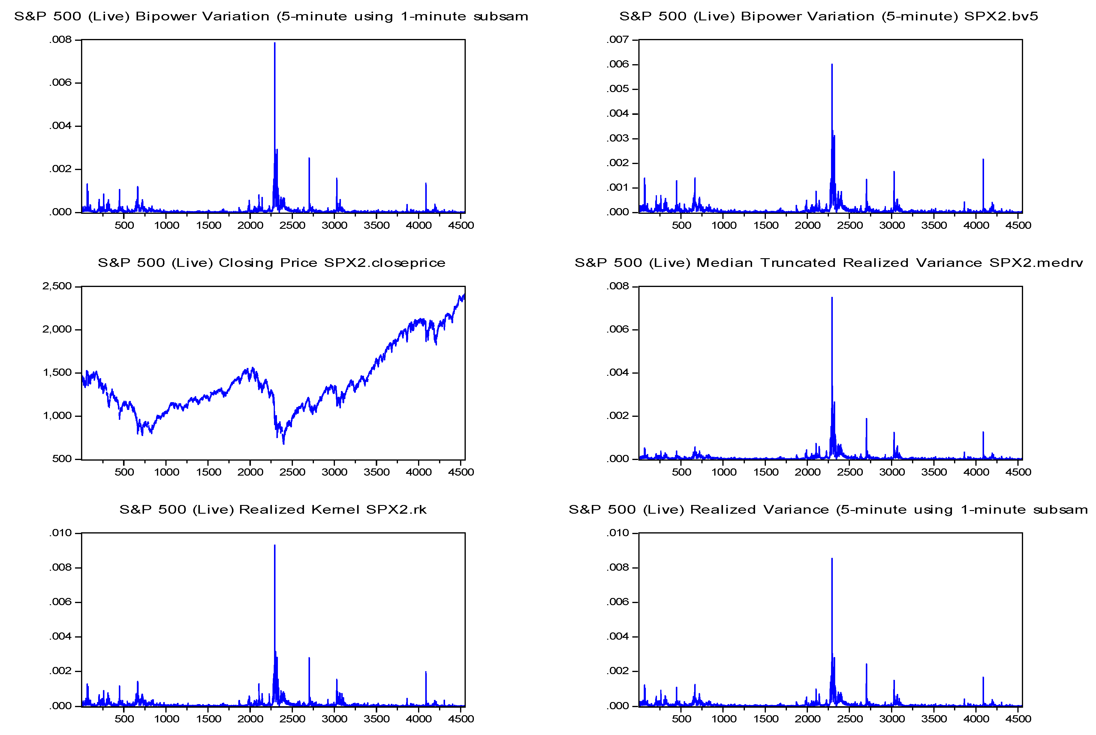](https://www.mdpi.com/jrfm/jrfm-13-00125/article_deploy/html/images/jrfm-13-00125-g001a.png)[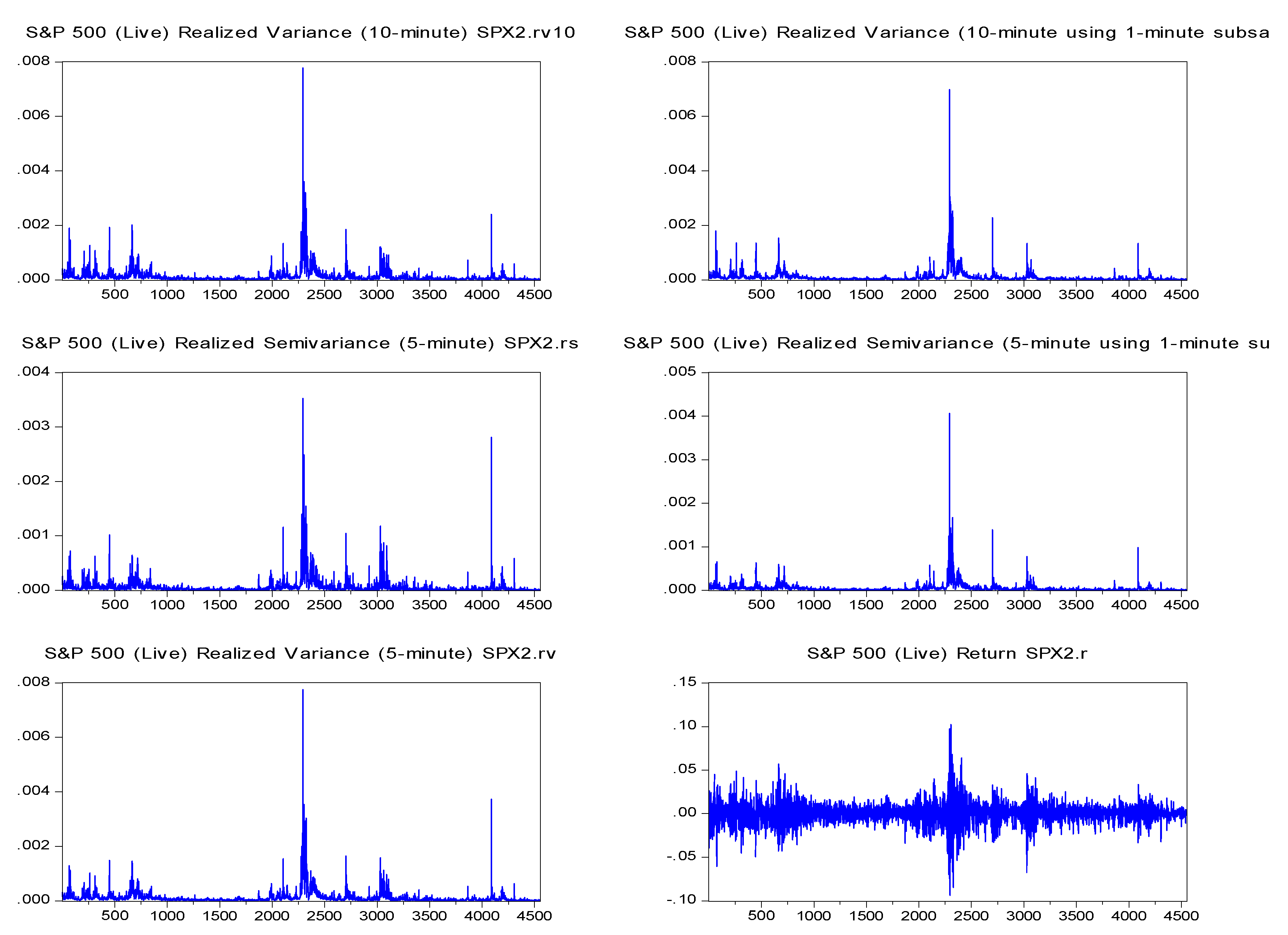](https://www.mdpi.com/jrfm/jrfm-13-00125/article_deploy/html/images/jrfm-13-00125-g001b.png)
**Figure 2.** FTSE100 plots. Note: This set of figures depict the realized measures on the FTSE100 index (from left to right): The first figure depicts the realized bi-power variation (5-min sub-sampled) estimator, the second figure depicts the realized bi-power variation (5-min) estimator, the third figure depicts the FTSE100 index closing price, the fourth figure depicts the median realized variance (5-min) estimator, the fifth figure depicts the realized Kernel variance estimator (two-scale/Barlett), the sixth figure depicts the realized variance (5-min sub-sampled) estimator, the seventh figure depicts the realized variance (10-min) estimator, the eighth figure depicts the realized variance (10-min sub-sampled) estimator, the ninth figure depicts the realized semi-variance (5-min) estimator, the tenth figure depicts the realized semi-variance (5-min sub-sampled) estimator, the eleventh figure depicts the realized variance (5-min) estimator, and the twelfth figure depicts the return of the FTSE100 index.
[](https://www.mdpi.com/jrfm/jrfm-13-00125/article_deploy/html/images/jrfm-13-00125-g002a.png)[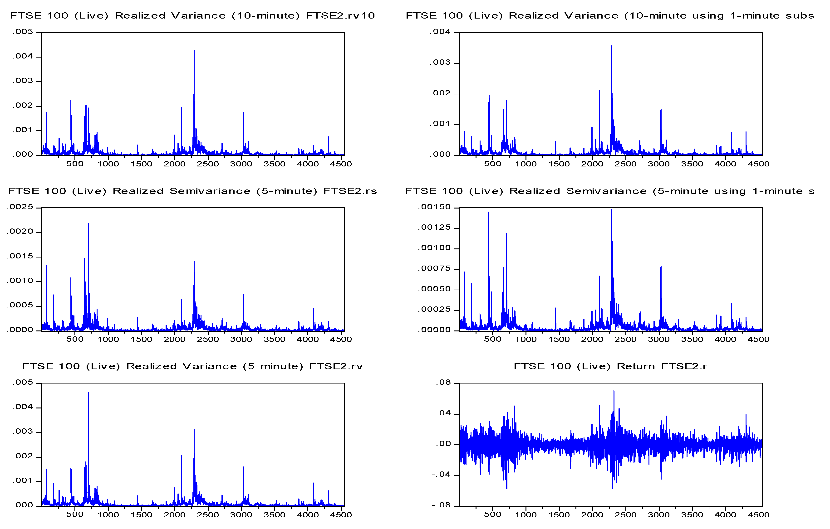](https://www.mdpi.com/jrfm/jrfm-13-00125/article_deploy/html/images/jrfm-13-00125-g002b.png)
**Figure 3.** Forecast errors plots. Note: This set of figures depicts the one-step-ahead forecast error of the expected returns in S\&P500 and FTSE100 indices used in this study obtained from a rolling-estimation window of 1000 observations.
[](https://www.mdpi.com/jrfm/jrfm-13-00125/article_deploy/html/images/jrfm-13-00125-g003.png)
**Figure 4.** Volatility regimes. Note: This set figures depicts the volatility regimes in returns and equity prices of S\&P500 and FTSE100 indices; the green color refers to high volatility regimes while the red color refers to low volatility regimes. Panel A refers to S\&P500 index sample. Panel B refers to FTSE100 index sample.
[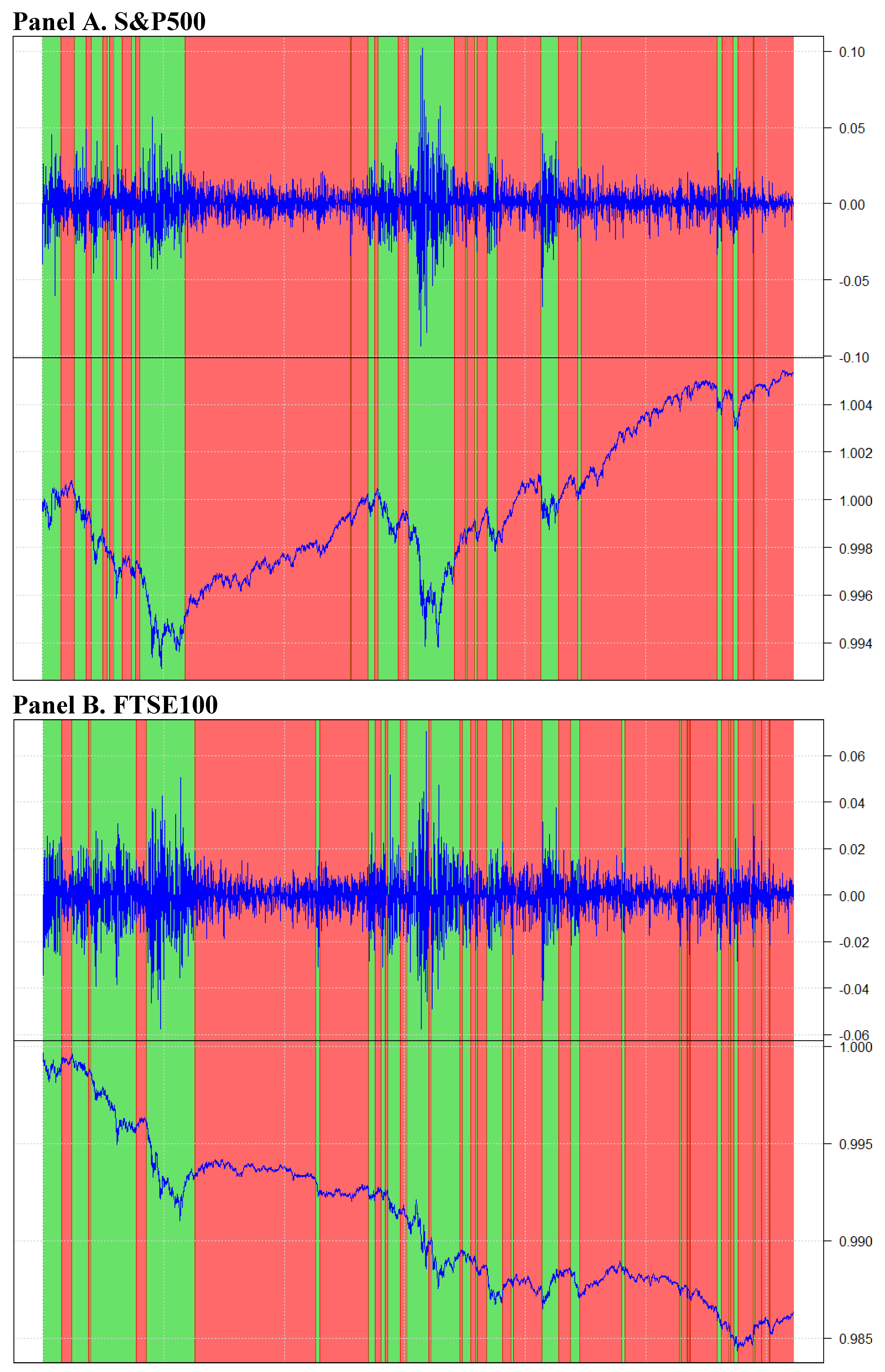](https://www.mdpi.com/jrfm/jrfm-13-00125/article_deploy/html/images/jrfm-13-00125-g004.png)
**Figure 5.** Defined volatility regimes. Note: This set figures depicts the volatility regimes in returns (upper figure) and the probability of the high and low volatility regimes (bottom figure) of S\&P500 and FTSE100 indices. On the bottom figure, the grey color refers to high volatility regimes while the black color refers to low volatility regimes. Panel A refers to S\&P500 index sample. Panel B refers to FTSE100 index sample.
[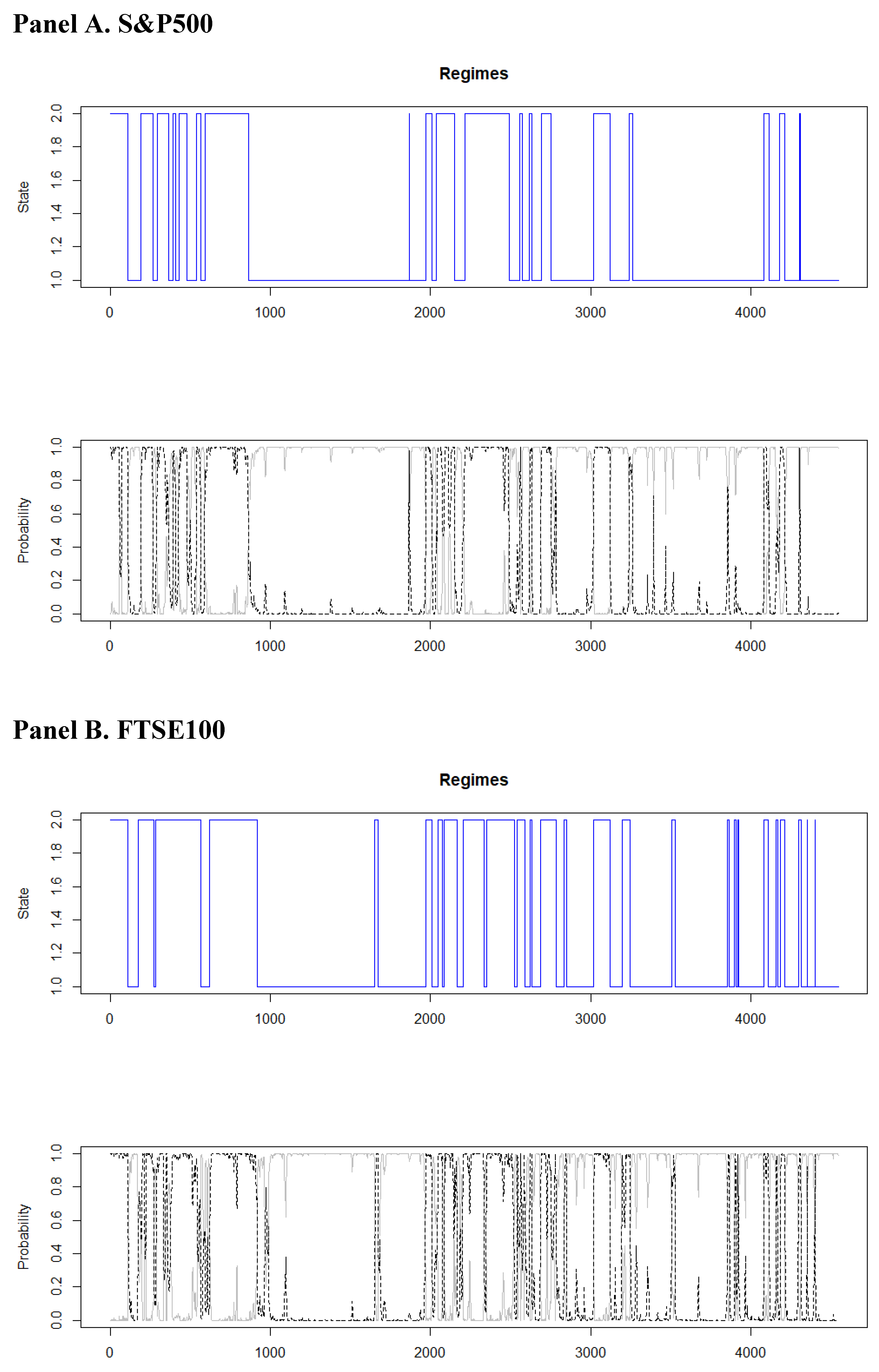](https://www.mdpi.com/jrfm/jrfm-13-00125/article_deploy/html/images/jrfm-13-00125-g005.png)
**Table 1.** Realized Estimators.
| Code | Description |
|---|---|
| 𝐵𝑃𝑉 B P V | Realized bi-power variation (5-min) |
| 𝐵𝑃𝑉𝑆𝑆 B P V S S | Realized bi-power variation (5-min sub-sampled) |
| 𝑀𝑒𝑑𝑅𝑉 M e d R V | Median realized variance (5-min) |
| 𝑅𝐾𝑃𝑎𝑟𝑧𝑒𝑛 R K P a r z e n | Realized Kernel variance (non-flat Parzen) |
| 𝑅𝐾𝑇𝐻2 R K T H 2 | Realized Kernel variance (Tukey-Hanning(2)) |
| 𝑅𝐾𝐵𝑎𝑟𝑙𝑒𝑡 R K B a r l e t | Realized Kernel variance (two-scale/Barlett) |
| 𝑅𝑆𝑉𝐷 R S V D | Realized downside semi-variance (5-min) |
| 𝑅𝑆𝑉𝐷,𝑆𝑆 R S V D , S S | Realized downside semi-variance (5-min sub-sampled) |
| 𝑅𝑉 R V | Realized variance |
| 𝑅𝑉10 R V 10 | Realized variance (10-min) |
| 𝑅𝑉𝑆𝑆10 R V 10 S S | Realized variance (10-min sub-sampled) |
| 𝑅𝑉5 R V 5 | Realized variance (5-min) |
| 𝑅𝑉𝑆𝑆5 R V 5 S S | Realized variance (5-min sub-sampled) |
Note: This table reports the list of realized estimators, codes, and full names of the 13 estimators of realized measures of three classes. The source of our data is the Oxford-Man Institute of Quantitative Finance. All realized measures require a choice of sampling frequency (e.g., 5-min or 10-min sampling), sampling scheme (calendar time or tick time), and whether to use transaction prices or mid-quotes.
**Table 2.** Hypothesis 1 (volatility feedback effect) regression results.
| Variable | Coefficient | Marginal Impact | Coefficient | Marginal Impact |
|---|---|---|---|---|
| | Panel A. S\&P500 | Panel B. FTSE100 | | |
| 𝐵𝑃𝑉 B P V | 24\.5036 \*\*\* | 0\.0037 | 14\.8874 | 0\.0010 |
| | (5.9560) | | (7.0660) | |
| 𝐵𝑃𝑉𝑆𝑆 B P V S S | 2\.4522 | 0\.0000 | 80\.1180 \*\*\* | 0\.0080 |
| | (13.1600) | | (13.2200) | |
| 𝑀𝑒𝑑𝑅𝑉 M e d R V | 53\.8661 \*\*\* | 0\.0307 | 41\.4710 \*\*\* | 0\.0231 |
| | (4.493) | | (4.003) | |
| 𝑅𝐾𝐵𝑎𝑟𝑙𝑒𝑡 R K B a r l e t | 20\.8178 \*\* | 0\.0012 | 1\.9995 | 0\.0000 |
| | (9.0300) | | (7.0130) | |
| 𝑅𝑆𝑉𝐷 R S V D | 174\.6970 \*\*\* | 0\.2244 | 121\.288 \*\*\* | 0\.0409 |
| | (4.8200) | | (8.712) | |
| 𝑅𝑆𝑉𝐷,𝑆𝑆 R S V D , S S | 147\.8110 \*\*\* | 0\.1341 | 89\.9744 \*\*\* | 0\.0184 |
| | (5.5730) | | (9.765) | |
| 𝑅𝑉 R V | 138\.2400 \*\*\* | 0\.0896 | 85\.2223 \*\*\* | 0\.0154 |
| | (6.5380) | | (10.1000) | |
| 𝑅𝑉10 R V 10 | 13\.5120 \*\*\* | 0\.0026 | 10\.6719 \*\* | 0\.0011 |
| | (3.9240) | | (4.7250) | |
| 𝑅𝑉𝑆𝑆10 R V 10 S S | 80\.5904 \*\*\* | 0\.0256 | 10\.4318 | 0\.0003 |
| | (7.383) | | (9.0230) | |
| 𝑅𝑉𝑆𝑆5 R V 5 S S | 183\.5250 \*\*\* | 0\.0256 | 157\.8510 \*\*\* | 0\.0226 |
| | (16.8100) | | (15.4000) | |
| c | 3\.0330 × 10−4 \* | 0\.0007 | 5\.9472 × 10−4 \*\*\* | 0\.0034 |
| | (1.6720 × 10⁻⁴) | | (1.5020 × 10⁻⁴) | |
| Obs. | 4552 | | 4552 | |
| R adj | 0\.7229 | | 0\.7436 | |
Note: This table reports the results of Hypothesis 1: Volatility feedback effect “If volatility is priced, does an anticipated increase in volatility raise the required return on equity, leading to an immediate stock price decline?”. The following estimators in absolute values are reported:
𝐵𝑃𝑉
B
P
V
is the realized bi-power variation (5-min) measure,
𝐵𝑃𝑉𝑆𝑆
B
P
V
S
S
is the realized bi-power variation (5-min sub-sampled) measure,
𝑀𝑒𝑑𝑅𝑉
M
e
d
R
V
is the median realized variance (5-min),
𝑅𝐾𝐵𝑎𝑟𝑙𝑒𝑡
R
K
B
a
r
l
e
t
is the realized Kernel variance (two-scale/Barlett),
𝑅𝑆𝑉𝐷
R
S
V
D
is the realized semi-variance (5-min),
𝑅𝑆𝑉𝐷,𝑆𝑆
R
S
V
D
,
S
S
is the realized semi-variance (5-min sub-sampled),
𝑅𝑉
R
V
is the realized volatility,
𝑅𝑉10
R
V
10
is the realized variance (10-min),
𝑅𝑉𝑆𝑆10
R
V
10
S
S
is the realized variance (10-min sub-sampled), and
𝑅𝑉𝑆𝑆5
R
V
5
S
S
is the realized variance (5-min sub-sampled). Standard errors are in parentheses. Panel A refers to the results from the S\&P500 index, and Panel B refers to the results from the FTSE100 index. \*\*\*, \*\* and \* indicate significance at 1, 5 and 10%, respectively.
**Table 3.** Hypothesis 2 (leverage effect) regression results.
| Variable | Coefficient | Marginal Impact | Coefficient | Marginal Impact |
|---|---|---|---|---|
| | Panel A. S\&P500 | Panel B. FTSE100 | | |
| 𝑅𝑡−1,𝑡 R t − 1 , t | −1.1040 × 10⁻³ \*\*\* | 0\.0068 | −5.6477 × 10⁻⁴ \*\*\* | 0\.0037 |
| | (1.9790 × 10⁻⁴) | | (1.3730 × 10⁻⁴) | |
| c | 1\.1636 × 10−4 | 0\.1755 | 8\.5092 × 10−5 \*\*\* | 0\.2158 |
| | (3.7350 × 10⁻⁶) | | (2.4060 × 10⁻⁶) | |
| Obs. | 4550 | | 4550 | |
| R-squared | 6\.7900 × 10−3 | | 3\.7000 × 10−3 | |
Note: This table reports the results of Hypothesis 2: Leverage effect “A drop in the value of the stock—negative return—increases financial leverage, which makes the stock riskier and increases its volatility?”. Standard errors are in parentheses. Panel A refers to the results from the S\&P500 index and Panel B refers to the results from the FTSE100 index. \*\*\* indicates significance at 1%.
**Table 4.** Estimation results in low and high volatility regimes.
| Low Volatility Regimes | High Volatility Regimes |
|---|---|
| **Panel A. S\&P500** | |
| 0\.8174 | 0\.8809 |
| 0\.8274 | 0\.8101 |
| 0\.7920 | 0\.7452 |
| 0\.7377 | 0\.7849 |
| 0\.7821 | 0\.7921 |
| **Panel B. FTSE100** | |
| 0\.6685 | 0\.7423 |
| 0\.6776 | 0\.7564 |
| 0\.7324 | 0\.7762 |
| 0\.6416 | 0\.8731 |
| 0\.7934 | 0\.7697 |
Note: This table reports the R adjusted (R adj) of Equation (8) for low and high volatility regimes. Panel A refers to S\&P500 index and Panel B refers to FTSE100 index. A total of 10 regimes (obtained by [Figure 4](https://www.mdpi.com/1911-8074/13/6/125#fig_body_display_jrfm-13-00125-f004) and [Figure 5](https://www.mdpi.com/1911-8074/13/6/125#fig_body_display_jrfm-13-00125-f005)) were picked, five lower volatility regimes and five higher volatility regimes (the selected regimes were the regimes with the higher number of observations).
| | |
|---|---|
| 1 | The relation between asset returns and expected volatility motivates the research to produce volatility forecast models using several techniques (see [Xu 1999](https://www.mdpi.com/1911-8074/13/6/125#B60-jrfm-13-00125); [Bali and Theodossiou 2007](https://www.mdpi.com/1911-8074/13/6/125#B9-jrfm-13-00125); [Wang and Zhu 2010](https://www.mdpi.com/1911-8074/13/6/125#B58-jrfm-13-00125); [Kiliç and Ugur 2018](https://www.mdpi.com/1911-8074/13/6/125#B45-jrfm-13-00125); [Shang et al. 2018](https://www.mdpi.com/1911-8074/13/6/125#B57-jrfm-13-00125); among others). |
| 2 | Our description is compact due to the fact that the details of the realized methodology used in this study have been laid out in recent contributions by [Gkillas](https://www.mdpi.com/1911-8074/13/6/125#B33-jrfm-13-00125) ([Gillas](https://www.mdpi.com/1911-8074/13/6/125#B33-jrfm-13-00125)) [et al.](https://www.mdpi.com/1911-8074/13/6/125#B33-jrfm-13-00125) ([2018](https://www.mdpi.com/1911-8074/13/6/125#B33-jrfm-13-00125)); [Demirer et al.](https://www.mdpi.com/1911-8074/13/6/125#B26-jrfm-13-00125) ([2019](https://www.mdpi.com/1911-8074/13/6/125#B26-jrfm-13-00125)); [Gkillas et al.](https://www.mdpi.com/1911-8074/13/6/125#B35-jrfm-13-00125) ([2019a](https://www.mdpi.com/1911-8074/13/6/125#B35-jrfm-13-00125), [2019b](https://www.mdpi.com/1911-8074/13/6/125#B36-jrfm-13-00125), [2020a](https://www.mdpi.com/1911-8074/13/6/125#B37-jrfm-13-00125), [2020b](https://www.mdpi.com/1911-8074/13/6/125#B38-jrfm-13-00125), [2020c](https://www.mdpi.com/1911-8074/13/6/125#B39-jrfm-13-00125)). |
© 2020 by the authors. Licensee MDPI, Basel, Switzerland. This article is an open access article distributed under the terms and conditions of the Creative Commons Attribution (CC BY) license (<http://creativecommons.org/licenses/by/4.0/>).
## Share and Cite
**MDPI and ACS Style**
Floros, C.; Gkillas, K.; Konstantatos, C.; Tsagkanos, A. Realized Measures to Explain Volatility Changes over Time. *J. Risk Financial Manag.* **2020**, *13*, 125. https://doi.org/10.3390/jrfm13060125
**AMA Style**
Floros C, Gkillas K, Konstantatos C, Tsagkanos A. Realized Measures to Explain Volatility Changes over Time. *Journal of Risk and Financial Management*. 2020; 13(6):125. https://doi.org/10.3390/jrfm13060125
**Chicago/Turabian Style**
Floros, Christos, Konstantinos Gkillas, Christoforos Konstantatos, and Athanasios Tsagkanos. 2020. "Realized Measures to Explain Volatility Changes over Time" *Journal of Risk and Financial Management* 13, no. 6: 125. https://doi.org/10.3390/jrfm13060125
**APA Style**
Floros, C., Gkillas, K., Konstantatos, C., & Tsagkanos, A. (2020). Realized Measures to Explain Volatility Changes over Time. *Journal of Risk and Financial Management*, *13*(6), 125. https://doi.org/10.3390/jrfm13060125
## Article Metrics
No

No
### Article Access Statistics
Created with Highcharts 4.0.4
Article access statistics
Article Views
26\. Dec
27\. Dec
28\. Dec
29\. Dec
30\. Dec
31\. Dec
1\. Jan
2\. Jan
3\. Jan
4\. Jan
5\. Jan
6\. Jan
7\. Jan
8\. Jan
9\. Jan
10\. Jan
11\. Jan
12\. Jan
13\. Jan
14\. Jan
15\. Jan
16\. Jan
17\. Jan
18\. Jan
19\. Jan
20\. Jan
21\. Jan
22\. Jan
23\. Jan
24\. Jan
25\. Jan
26\. Jan
27\. Jan
28\. Jan
29\. Jan
30\. Jan
31\. Jan
1\. Feb
2\. Feb
3\. Feb
4\. Feb
5\. Feb
6\. Feb
7\. Feb
8\. Feb
9\. Feb
10\. Feb
11\. Feb
12\. Feb
13\. Feb
14\. Feb
15\. Feb
16\. Feb
17\. Feb
18\. Feb
19\. Feb
20\. Feb
21\. Feb
22\. Feb
23\. Feb
24\. Feb
25\. Feb
26\. Feb
27\. Feb
28\. Feb
1\. Mar
2\. Mar
3\. Mar
4\. Mar
5\. Mar
6\. Mar
7\. Mar
8\. Mar
9\. Mar
10\. Mar
11\. Mar
12\. Mar
13\. Mar
14\. Mar
15\. Mar
16\. Mar
17\. Mar
18\. Mar
19\. Mar
20\. Mar
21\. Mar
22\. Mar
23\. Mar
24\. Mar
25\. Mar
0k
2k
4k
6k
8k
For more information on the journal statistics, click [here](https://www.mdpi.com/journal/jrfm/stats).
Multiple requests from the same IP address are counted as one view.
[Zoom]() \| [Orient]() \| [As Lines]() \| [As Sticks]() \| [As Cartoon]() \| [As Surface]() \| [Previous Scene]() \| [Next Scene]()
## Cite
Export citation file: [BibTeX]() \| [EndNote]() \| [RIS]()
**MDPI and ACS Style**
Floros, C.; Gkillas, K.; Konstantatos, C.; Tsagkanos, A. Realized Measures to Explain Volatility Changes over Time. *J. Risk Financial Manag.* **2020**, *13*, 125. https://doi.org/10.3390/jrfm13060125
**AMA Style**
Floros C, Gkillas K, Konstantatos C, Tsagkanos A. Realized Measures to Explain Volatility Changes over Time. *Journal of Risk and Financial Management*. 2020; 13(6):125. https://doi.org/10.3390/jrfm13060125
**Chicago/Turabian Style**
Floros, Christos, Konstantinos Gkillas, Christoforos Konstantatos, and Athanasios Tsagkanos. 2020. "Realized Measures to Explain Volatility Changes over Time" *Journal of Risk and Financial Management* 13, no. 6: 125. https://doi.org/10.3390/jrfm13060125
**APA Style**
Floros, C., Gkillas, K., Konstantatos, C., & Tsagkanos, A. (2020). Realized Measures to Explain Volatility Changes over Time. *Journal of Risk and Financial Management*, *13*(6), 125. https://doi.org/10.3390/jrfm13060125
[*clear*]()
*[J. Risk Financial Manag.](https://www.mdpi.com/journal/jrfm)*, EISSN 1911-8074, Published by MDPI
[RSS](https://www.mdpi.com/rss/journal/jrfm) [Content Alert](https://www.mdpi.com/journal/jrfm/toc-alert)
### Further Information
[Article Processing Charges](https://www.mdpi.com/apc) [Pay an Invoice](https://www.mdpi.com/about/payment) [Open Access Policy](https://www.mdpi.com/openaccess) [Contact MDPI](https://www.mdpi.com/about/contact) [Jobs at MDPI](https://careers.mdpi.com/)
### Guidelines
[For Authors](https://www.mdpi.com/authors) [For Reviewers](https://www.mdpi.com/reviewers) [For Editors](https://www.mdpi.com/editors) [For Librarians](https://www.mdpi.com/librarians) [For Publishers](https://www.mdpi.com/publishing_services) [For Societies](https://www.mdpi.com/societies) [For Conference Organizers](https://www.mdpi.com/conference_organizers)
### MDPI Initiatives
[Sciforum](https://sciforum.net/) [MDPI Books](https://www.mdpi.com/books) [Preprints.org](https://www.preprints.org/) [Scilit](https://www.scilit.com/) [SciProfiles](https://sciprofiles.com/?utm_source=mpdi.com&utm_medium=bottom_menu&utm_campaign=initiative) [Encyclopedia](https://encyclopedia.pub/) [JAMS](https://jams.pub/) [Proceedings Series](https://www.mdpi.com/about/proceedings)
### Follow MDPI
[LinkedIn](https://www.linkedin.com/company/mdpi) [Facebook](https://www.facebook.com/MDPIOpenAccessPublishing) [X](https://x.com/MDPIOpenAccess)

© 1996-2026 MDPI (Basel, Switzerland) unless otherwise stated
[Disclaimer]()
Disclaimer/Publisher’s Note: The statements, opinions and data contained in all publications are solely those of the individual author(s) and contributor(s) and not of MDPI and/or the editor(s). MDPI and/or the editor(s) disclaim responsibility for any injury to people or property resulting from any ideas, methods, instructions or products referred to in the content.
[Terms and Conditions](https://www.mdpi.com/about/terms-and-conditions) [Privacy Policy](https://www.mdpi.com/about/privacy)
We use cookies on our website to ensure you get the best experience.
Read more about our cookies [here](https://www.mdpi.com/about/privacy).
[Accept](https://www.mdpi.com/accept_cookies)
## Share Link
[Copy]()
[*clear*]()
## Share
https://www.mdpi.com/742304
[*clear*]()
[Back to TopTop](https://www.mdpi.com/1911-8074/13/6/125) |
| Readable Markdown | ## 1\. Introduction
Asset pricing in financial literature is predicated on the importance of volatility in asset returns. Hence, financial market volatility is a key factor ranging from investment decisions to derivatives pricing and financial market regulation ([Poon and Granger 2003](https://www.mdpi.com/1911-8074/13/6/125#B54-jrfm-13-00125)). Volatility, as a measure of market risk, is always an anxiety-generating factor for market participants not only in terms of its nature but also its level ([Giot et al. 2010](https://www.mdpi.com/1911-8074/13/6/125#B32-jrfm-13-00125)). Admittedly, volatility is an unobservable variable and its effects on financial markets are hard to anticipate. This is one of the reasons that asset return volatilities (henceforth, volatility) are of utmost importance to empirical finance. In other words, it remains the ingredient in assessing asset or portfolio risk, playing an important role in asset pricing models which heavily depend on underlying asset return dynamics. Asset management and asset pricing models require the proper volatility modeling of financial assets.
The existing literature has laid emphasis on time-varying volatility suggesting various tools for its modeling (see [Andersen and Bollerslev 1998](https://www.mdpi.com/1911-8074/13/6/125#B2-jrfm-13-00125); [Andersen et al. 2001a](https://www.mdpi.com/1911-8074/13/6/125#B3-jrfm-13-00125); [Barndorff-Nielsen and Shephard 2002](https://www.mdpi.com/1911-8074/13/6/125#B10-jrfm-13-00125), [2004](https://www.mdpi.com/1911-8074/13/6/125#B11-jrfm-13-00125); [Andersen et al. 2007](https://www.mdpi.com/1911-8074/13/6/125#B5-jrfm-13-00125); [Barndorff-Nielsen et al. 2008](https://www.mdpi.com/1911-8074/13/6/125#B13-jrfm-13-00125); [Hansen and Horel 2009](https://www.mdpi.com/1911-8074/13/6/125#B41-jrfm-13-00125); [Meddahi et al. 2011](https://www.mdpi.com/1911-8074/13/6/125#B51-jrfm-13-00125); [Alghalith et al. 2020](https://www.mdpi.com/1911-8074/13/6/125#B1-jrfm-13-00125); among others). [Andersen and Bollerslev](https://www.mdpi.com/1911-8074/13/6/125#B2-jrfm-13-00125) ([1998](https://www.mdpi.com/1911-8074/13/6/125#B2-jrfm-13-00125)) showed that ARCH models produce strikingly accurate inter-daily forecasts for the latent volatility on most financial applications. [Andersen et al.](https://www.mdpi.com/1911-8074/13/6/125#B3-jrfm-13-00125) ([2001a](https://www.mdpi.com/1911-8074/13/6/125#B3-jrfm-13-00125)) found evidence that realized volatilities and correlations move together in a manner broadly consistent with latent factor structure. [Barndorff-Nielsen and Shephard](https://www.mdpi.com/1911-8074/13/6/125#B10-jrfm-13-00125) ([2002](https://www.mdpi.com/1911-8074/13/6/125#B10-jrfm-13-00125)) used quadratic variation-like measures of activity in financial markets, called realized volatility, to investigate the stochastic properties of returns. [Barndorff-Nielsen and Shephard](https://www.mdpi.com/1911-8074/13/6/125#B11-jrfm-13-00125) ([2004](https://www.mdpi.com/1911-8074/13/6/125#B11-jrfm-13-00125)) suggested that, in special cases, realized bi-power variation estimates integrated variance in stochastic volatility models, providing a model-free and consistent alternative to realized variance. [Andersen et al.](https://www.mdpi.com/1911-8074/13/6/125#B5-jrfm-13-00125) ([2007](https://www.mdpi.com/1911-8074/13/6/125#B5-jrfm-13-00125)) used high frequency futures dataset to investigate the effects on the financial market volatility; they concluded that news produces conditional mean jumps. [Barndorff-Nielsen et al.](https://www.mdpi.com/1911-8074/13/6/125#B13-jrfm-13-00125) ([2008](https://www.mdpi.com/1911-8074/13/6/125#B13-jrfm-13-00125)) used realized kernels to investigate efficient feasible inference on the ex post variation of underlying equity prices in the presence of simple models of market frictions. [Hansen and Horel](https://www.mdpi.com/1911-8074/13/6/125#B41-jrfm-13-00125) ([2009](https://www.mdpi.com/1911-8074/13/6/125#B41-jrfm-13-00125)) suggested an estimator of the quadratic variation, removing the effects of market microstructure noise, which is based on the theory of Markov chains and consistent with a Gaussian limit distribution.
Despite extensive studies on the relation between volatility and expected returns ([Campbell and Hentschel 1992](https://www.mdpi.com/1911-8074/13/6/125#B20-jrfm-13-00125); [Glosten et al. 1993](https://www.mdpi.com/1911-8074/13/6/125#B40-jrfm-13-00125); [Ang et al. 2006](https://www.mdpi.com/1911-8074/13/6/125#B8-jrfm-13-00125)), the literature establishes empirical evidence of the existence of a link between asset returns and expected volatility, as volatility is associated with volatility risk premium.[1](https://www.mdpi.com/1911-8074/13/6/125#fn001-jrfm-13-00125) In particular, volatility risk premium as a part of asset price can be linked to expected volatility either through risk-premium or leverage-effect ([Christie 1982](https://www.mdpi.com/1911-8074/13/6/125#B22-jrfm-13-00125)). However, little has been done in examining jointly how realized volatility affects returns and vice versa. [Bollerslev and Zhou](https://www.mdpi.com/1911-8074/13/6/125#B18-jrfm-13-00125) ([2006](https://www.mdpi.com/1911-8074/13/6/125#B18-jrfm-13-00125)) provided theoretical framework for assessing the empirical linkages between returns and realized and implied volatility. We investigate the empirical linkages between returns and various realized volatility measures. In doing so, we extend previous works (e.g., [Bollerslev and Zhou 2006](https://www.mdpi.com/1911-8074/13/6/125#B18-jrfm-13-00125)) on this topic by considering recent data from the most common benchmarks for the broader US and UK equity markets, namely the Standard & Poor’s 500 Index (S\&P500) and the Financial Times Stock Exchange 100 Index (FTSE100) indices.
According to [Bekaert and Wu](https://www.mdpi.com/1911-8074/13/6/125#B16-jrfm-13-00125) ([2000](https://www.mdpi.com/1911-8074/13/6/125#B16-jrfm-13-00125)), and [Black](https://www.mdpi.com/1911-8074/13/6/125#B17-jrfm-13-00125) ([1976](https://www.mdpi.com/1911-8074/13/6/125#B17-jrfm-13-00125)), two research questions arise respectively:
> Q1: “If volatility is priced, does an anticipated increase in volatility raise the required return on equity, leading to an immediate stock price decline?”
> Q2: “Does a drop in the value of the stock (negative return) increase financial leverage, so that it makes the stock riskier and increases its volatility?”.
To give full answers to the above questions, we empirically examine the magnitude and the sign of the linear relationship between market-based volatility and contemporaneous returns, the so-called volatility feedback effect both on S\&P500 and FTSE100. Consequently, we study (1) the existence of positive relationship market-based volatility and contemporaneous returns and (2) the existence of negative relationship between the lagged returns and the volatility. According to [Carr and Wu](https://www.mdpi.com/1911-8074/13/6/125#B21-jrfm-13-00125) ([2017](https://www.mdpi.com/1911-8074/13/6/125#B21-jrfm-13-00125)), “this effect can show up as a negative correlation between the index return and its volatility, regardless of the market’s financial leverage level”. Furthermore, we test the relationship between the lagged returns and the current market-based volatility, the so-called leverage effect. We refer to the study implemented by [Zumbach](https://www.mdpi.com/1911-8074/13/6/125#B63-jrfm-13-00125) ([2013](https://www.mdpi.com/1911-8074/13/6/125#B63-jrfm-13-00125)) for a detailed analysis of the leverage effect. The literature often refers to a negative relation between equity return and return volatility as a “leverage effect” ([Carr and Wu 2017](https://www.mdpi.com/1911-8074/13/6/125#B21-jrfm-13-00125)).
In this paper, we provide empirical results from intraday data to derive a negative relation between returns and volatilities; to the best of our knowledge, this is the first study that considers several realized measures to explain these hypotheses. Asset management and asset pricing models require a proper volatility modeling of financial assets. High frequency data contains more information about the market, such as the intraday changes and the market microstructure, making realized measures more accurate than those constructed by employing lower frequencies (see [Hansen and Huang 2016](https://www.mdpi.com/1911-8074/13/6/125#B42-jrfm-13-00125)). For modelling volatility with high-frequency data, see [Degiannakis and Floros](https://www.mdpi.com/1911-8074/13/6/125#B24-jrfm-13-00125) ([2015](https://www.mdpi.com/1911-8074/13/6/125#B24-jrfm-13-00125)). However, market participants face problems when modelling volatility using intraday data. They should choose the correct sampling frequency as well as whether to sample prices in calendar time (every n seconds) or tick time (every m trades). Nevertheless, when both quotation prices and transaction are available, the selection of which price to use arises too. What is more, some realized measures require selections about tuning parameters, such as kernel bandwidth. All realized measures are based on the minute-by-minute intraday data of S\&P500 (US) and FTSE100 (UK) indices.
For the analysis, we examined a large number of realized measures across S\&P500 and FTSE100 indices, we considered thirteen realized estimators from three classes, and we applied these to 17 years of data. Our objective was to compare a large number of available realized measures to examine the volatility and leverage effects, providing a comparison of realized measures in environments with varied price processes and market microstructures. The existing literature shows that realized measures estimated by high frequency data are the most appropriate tools to deal with good and bad volatility (see [Degiannakis and Floros 2015](https://www.mdpi.com/1911-8074/13/6/125#B24-jrfm-13-00125), [2016](https://www.mdpi.com/1911-8074/13/6/125#B25-jrfm-13-00125)). The importance of the examination of volatility can also emerge from upside and downside volatility associated the positive and negative price increments (see [Bollerslev et al. 2019](https://www.mdpi.com/1911-8074/13/6/125#B19-jrfm-13-00125)). In volatility modeling, it is necessary to decompose the volatility into two parts, the perceived as directional-persistent volatility (good volatility) and the jumpy-relatively hard to anticipate volatility (bad volatility; see [Giot et al. 2010](https://www.mdpi.com/1911-8074/13/6/125#B32-jrfm-13-00125)). As a consequence, many estimators of asset return volatility constructed using high-frequency price data have been suggested by [Andersen and Bollerslev](https://www.mdpi.com/1911-8074/13/6/125#B2-jrfm-13-00125) ([1998](https://www.mdpi.com/1911-8074/13/6/125#B2-jrfm-13-00125)), [Andersen et al.](https://www.mdpi.com/1911-8074/13/6/125#B3-jrfm-13-00125) ([2001a](https://www.mdpi.com/1911-8074/13/6/125#B3-jrfm-13-00125)), [Barndorff-Nielsen and Shephard](https://www.mdpi.com/1911-8074/13/6/125#B10-jrfm-13-00125) ([2002](https://www.mdpi.com/1911-8074/13/6/125#B10-jrfm-13-00125), [2004](https://www.mdpi.com/1911-8074/13/6/125#B11-jrfm-13-00125)), [Andersen et al.](https://www.mdpi.com/1911-8074/13/6/125#B5-jrfm-13-00125) ([2007](https://www.mdpi.com/1911-8074/13/6/125#B5-jrfm-13-00125)), [Barndorff-Nielsen et al.](https://www.mdpi.com/1911-8074/13/6/125#B13-jrfm-13-00125) ([2008](https://www.mdpi.com/1911-8074/13/6/125#B13-jrfm-13-00125)), [Hansen and Horel](https://www.mdpi.com/1911-8074/13/6/125#B41-jrfm-13-00125) ([2009](https://www.mdpi.com/1911-8074/13/6/125#B41-jrfm-13-00125)), and [Meddahi et al.](https://www.mdpi.com/1911-8074/13/6/125#B51-jrfm-13-00125) ([2011](https://www.mdpi.com/1911-8074/13/6/125#B51-jrfm-13-00125)), among others; these include realized variance, realized bi-power variation, and median realized variance. In this study, we also considered a simple realized variance estimator with a reasonable choice of sampling frequency, namely the 5-min realized variance or 10-min realized variance, and tested whether it was a “good” estimator, following the recent literature (see [Gkillas et al. 2019b](https://www.mdpi.com/1911-8074/13/6/125#B36-jrfm-13-00125)). As both frequencies are “good” to construct realized estimators, [Liu et al.](https://www.mdpi.com/1911-8074/13/6/125#B46-jrfm-13-00125) ([2015](https://www.mdpi.com/1911-8074/13/6/125#B46-jrfm-13-00125)) found that the adequate balance between high and low sampling frequencies vary across different assets. However, the comparison of estimation accuracy shows that “it is difficult to significantly beat RV 5 estimator” ([Liu et al. 2015](https://www.mdpi.com/1911-8074/13/6/125#B46-jrfm-13-00125)); in this paper we also used the realized bi-power variation and median realized variance to deal with good volatility. On the other hand, [Low et al.](https://www.mdpi.com/1911-8074/13/6/125#B48-jrfm-13-00125) ([2016](https://www.mdpi.com/1911-8074/13/6/125#B48-jrfm-13-00125)) found that, by using copula-based models, several mean–variance-based rules exhibit statistically significant and superior performance improvements. For the superior performance of portfolio optimization, they follow [Low](https://www.mdpi.com/1911-8074/13/6/125#B47-jrfm-13-00125) ([2018](https://www.mdpi.com/1911-8074/13/6/125#B47-jrfm-13-00125)) by applying the Clayton canonical vine copula. For pairs trading strategy, see [Rad et al.](https://www.mdpi.com/1911-8074/13/6/125#B55-jrfm-13-00125) ([2016](https://www.mdpi.com/1911-8074/13/6/125#B55-jrfm-13-00125)).
The results for the S\&P500 index show that eight estimators explain approximately 72% of the returns of the S\&P500 index. As for the FTSE100 index, six estimators explain approximately 74% of the returns of the FTSE100 index. Also, in both indices, the returns negatively affect the realized volatility. Such findings are recommended to high-frequency financial analysts and volatility modelers. The findings are robust, using not only several realized measures estimated by high frequency data, but also using different sub-samples, providing evidence that realized measures have significantly impacted on return and vice versa.
This paper is organized as follows: [Section 2](https://www.mdpi.com/1911-8074/13/6/125#sec2-jrfm-13-00125) details the data selection and introduces the realized measures used in this study. [Section 3](https://www.mdpi.com/1911-8074/13/6/125#sec3-jrfm-13-00125) introduces the hypotheses and discusses the estimation results. [Section 4](https://www.mdpi.com/1911-8074/13/6/125#sec4-jrfm-13-00125) discuss further practical implications of the results. [Section 5](https://www.mdpi.com/1911-8074/13/6/125#sec5-jrfm-13-00125) concludes by summarizing the results of this study.
## 2\. Data and Methodology
In this section, we present the methodology used to compute the realized measures and provide the data and data adjustment.
### 2\.1. Realized Measures
We first provide some theoretical considerations of the realized volatility estimators. Second, we present the methodology of construction realized measures, and thus we classify the realized measures considered in this study into three classes.[2](https://www.mdpi.com/1911-8074/13/6/125#fn002-jrfm-13-00125)
#### 2\.1.1. Theoretical Considerations
Realized measures are theoretically sound high frequency, nonparametric estimators of the variation of the price path of an asset during the times at which the asset trades frequently on an index. The background to realized measures can be found in the survey articles by [McAleer and Medeiros](https://www.mdpi.com/1911-8074/13/6/125#B50-jrfm-13-00125) ([2008](https://www.mdpi.com/1911-8074/13/6/125#B50-jrfm-13-00125)) and [Barndorff-Nielsen and Shephard](https://www.mdpi.com/1911-8074/13/6/125#B12-jrfm-13-00125) ([2006](https://www.mdpi.com/1911-8074/13/6/125#B12-jrfm-13-00125)).
In this section, we present the theory of quadratic variation ( Q V ). For discrete prices process, the volatility at the given time of trade t can be estimated by quadratic variation ( Q V ) as:
Q V t \= ∫ t − 1 t σ s 2 d s \+ ∑ t − 1 \< s ≤ t κ s 2 t
(1)
where ∫ t − 1 t σ s 2 d s denotes the continuous variation and ∑ t − 1 \< s ≤ t κ s 2 t denotes the discontinuous variation. The Q V is considered as a biased estimator of integrated volatility.
Under weak regularity conditions and as N → ∞, realized volatility R V is a consistent estimator of quadratic variation Q V t:
R V t → N → ∞ Q V t
(2)
Following [Barndorff-Nielsen and Shephard](https://www.mdpi.com/1911-8074/13/6/125#B11-jrfm-13-00125) ([2004](https://www.mdpi.com/1911-8074/13/6/125#B11-jrfm-13-00125), [2006](https://www.mdpi.com/1911-8074/13/6/125#B12-jrfm-13-00125)), the quadratic variation is separated into its continuous and discontinuous components. The continuous sample path variation ∫ t − 1 t σ s 2 d s can be estimated by the realized bi-power variation ( B P V ) or by the median realized variance ( M R V ). The difference between realized variance and realized bi-power variation estimates the discontinuous component ∑ t − 1 \< s ≤ t κ s 2 t of the quadratic variation ([Barndorff-Nielsen and Shephard 2004](https://www.mdpi.com/1911-8074/13/6/125#B11-jrfm-13-00125)).
#### 2\.1.2. Classes of Realized Measures
First class includes the measures on realized variance (R V) constructed as the sum of squared intraday returns introduced by [Andersen et al.](https://www.mdpi.com/1911-8074/13/6/125#B4-jrfm-13-00125) ([2001b](https://www.mdpi.com/1911-8074/13/6/125#B4-jrfm-13-00125)). Under certain conditions on the market microstructure noise, these estimators are consistent at the optimal rate ([Liu et al. 2015](https://www.mdpi.com/1911-8074/13/6/125#B46-jrfm-13-00125)). The realized variance is given by:
R V t \= ∑ i \= 1 N r i , t 2
(3)
However, R V estimator is a consistent nonparametric estimator (see [Barndorff-Nielsen and Shephard 2002](https://www.mdpi.com/1911-8074/13/6/125#B10-jrfm-13-00125)). [Hansen and Lunde](https://www.mdpi.com/1911-8074/13/6/125#B43-jrfm-13-00125) ([2006](https://www.mdpi.com/1911-8074/13/6/125#B43-jrfm-13-00125)) concluded that R V estimator is biased at high frequency sampling. This class also includes the two-scale realized variance (T S R V) and the multi-scale realized variance (M S R V) introduced by [Zhang et al.](https://www.mdpi.com/1911-8074/13/6/125#B62-jrfm-13-00125) ([2005](https://www.mdpi.com/1911-8074/13/6/125#B62-jrfm-13-00125)) and [Zhang](https://www.mdpi.com/1911-8074/13/6/125#B61-jrfm-13-00125) ([2006](https://www.mdpi.com/1911-8074/13/6/125#B61-jrfm-13-00125)), respectively. These estimators are a combination of subsampled R V on slower frequency sampling and R V on higher frequency sampling.
To capture the sign asymmetry of the price process, the downside and upside semi-variance (realized volatility) are constructed. Following [Barndorff-Nielsen et al.](https://www.mdpi.com/1911-8074/13/6/125#B15-jrfm-13-00125) ([2010](https://www.mdpi.com/1911-8074/13/6/125#B15-jrfm-13-00125)), the downside realized semi-variance (R S V t D) can be defined as:
R S V t D \= ∑ i \= 1 N r i , t 2 I { r i , t \< 0 }
(4)
Second class is a generalization of realized volatility R V. It includes realized kernel (R K) estimators introduced by [Barndorff-Nielsen et al.](https://www.mdpi.com/1911-8074/13/6/125#B13-jrfm-13-00125) ([2008](https://www.mdpi.com/1911-8074/13/6/125#B13-jrfm-13-00125)). This class includes three realized measures using several different kernels; first R K with the “two-scale” (R K B a r l e t) Bartlett estimator, second the modified Tukey-Hanning kernel (R K T H 2) estimator, and third the “non-flat” Parzen (R K P a r z e n) estimator. All estimators fit a wider variety of microstructure effects (i.e., noise), leading to consistent estimators.
Following [Barndorff-Nielsen et al.](https://www.mdpi.com/1911-8074/13/6/125#B13-jrfm-13-00125) ([2008](https://www.mdpi.com/1911-8074/13/6/125#B13-jrfm-13-00125)), realized measures using several different kernels can be defined as:
R K t \= ∑ h \= − H H k ( h / ( H \+ 1 ) ) γ h
(5)
where γ h \= ∑ j \= \| h \| \+ 1 n r t , j r t , j − \| h \| and k ( x ) is a kernel weight function such that k ( 0 ) \= 1 and k ( 1 ) \= 0 and the optimal bandwidth parameter H is estimated using the procedure of [Barndorff-Nielsen et al.](https://www.mdpi.com/1911-8074/13/6/125#B14-jrfm-13-00125) ([2009](https://www.mdpi.com/1911-8074/13/6/125#B14-jrfm-13-00125)). The realized kernel measure is guaranteed to be non-negative, which is quite important, as some of our time series methods rely on this property. The first special case of the so-called flat-top Bartlett kernel defined where k ( x ) \= ( 1 − x ) is particularly interesting as its asymptotic distribution is the same as that of the two-scale estimator. The second special case of the so-called Tukey–Hanning defined where k h p ( x ) \= s i n 2 ( π 2 ( 1 − x ) p ).
Third class are the jump-robust realized measures as bi-power variation ( B P V ) introduced by [Barndorff-Nielsen and Shephard](https://www.mdpi.com/1911-8074/13/6/125#B12-jrfm-13-00125) ([2006](https://www.mdpi.com/1911-8074/13/6/125#B12-jrfm-13-00125)), which is a scaled sum of products of adjacent absolute returns and the median realized variance ( M e d R V ) estimator introduced by [Andersen et al.](https://www.mdpi.com/1911-8074/13/6/125#B7-jrfm-13-00125) ([2012](https://www.mdpi.com/1911-8074/13/6/125#B7-jrfm-13-00125)), which is a scaled square of the median of three consecutive intraday absolute returns. As B P V is influenced by the sampling frequency, M e d R V is characterized as a more robust estimator to jumps and microstructure noise than B P V (see [Barndorff-Nielsen and Shephard 2004](https://www.mdpi.com/1911-8074/13/6/125#B11-jrfm-13-00125); [Andersen et al. 2012](https://www.mdpi.com/1911-8074/13/6/125#B7-jrfm-13-00125)).
[Barndorff-Nielsen and Shephard](https://www.mdpi.com/1911-8074/13/6/125#B11-jrfm-13-00125) ([2004](https://www.mdpi.com/1911-8074/13/6/125#B11-jrfm-13-00125), [2006](https://www.mdpi.com/1911-8074/13/6/125#B12-jrfm-13-00125)) separated the quadratic variation into its continuous and discontinuous components. The continuous part of Q V can be estimated by the realized bi-power variation B P V t as follows:
B P V t \= μ 1 − 2 N N − 2 ∑ j − 3 N \| r i − 1 , t \| \| r i , t \|
(6)
where μ α is equal to E ( \| Z \| α ), where Z ∼ N ( 0 , 1 ) and α \> 0, thus μ 1 is equal to 2 / π. [Andersen et al.](https://www.mdpi.com/1911-8074/13/6/125#B7-jrfm-13-00125) ([2012](https://www.mdpi.com/1911-8074/13/6/125#B7-jrfm-13-00125)) proposed the median realized variance M e d R V t as the robust estimator instead of B P V t.
[Andersen et al.](https://www.mdpi.com/1911-8074/13/6/125#B7-jrfm-13-00125) ([2012](https://www.mdpi.com/1911-8074/13/6/125#B7-jrfm-13-00125)) proposed the median realized variance M e d R V t as a robust estimator to test the continuous variation which attenuates the effect of noise, instead of B P V t which is influenced by the sampling frequency.
M e d R V t \= π 6 − 4 3 \+ π ( N N − 2 ) ∑ i \= 1 N − 1 med ( \| r i − 1 , t \| , \| r i . t \| , \| r i \+ 1 , t \| ) 2
(7)
Three estimators which are somewhat robust to market microstructure noise have been suggested in the following literature: pre-averaging by [Jacod](https://www.mdpi.com/1911-8074/13/6/125#B44-jrfm-13-00125) ([2007](https://www.mdpi.com/1911-8074/13/6/125#B44-jrfm-13-00125)), multi-scale by [Zhang et al.](https://www.mdpi.com/1911-8074/13/6/125#B62-jrfm-13-00125) ([2005](https://www.mdpi.com/1911-8074/13/6/125#B62-jrfm-13-00125)) and [Zhang](https://www.mdpi.com/1911-8074/13/6/125#B61-jrfm-13-00125) ([2006](https://www.mdpi.com/1911-8074/13/6/125#B61-jrfm-13-00125)) and realized kernel by [Barndorff-Nielsen et al.](https://www.mdpi.com/1911-8074/13/6/125#B13-jrfm-13-00125) ([2008](https://www.mdpi.com/1911-8074/13/6/125#B13-jrfm-13-00125)).
### 2\.2. Data and Data Adjustments
We followed [Patton](https://www.mdpi.com/1911-8074/13/6/125#B53-jrfm-13-00125) ([2011](https://www.mdpi.com/1911-8074/13/6/125#B53-jrfm-13-00125)) by using the data-based ranking method. This method makes no assumption with regard to the market microstructure noise properties, apart from standard moment and mixing conditions. In this study on the relative performance of estimators of intraday quadratic variation from three classes of realized measures, we used transactions and quotation prices from January 2000 to June 2017, sampled in calendar time and tick-time, for sampling frequencies ranging from 5-min to 10-min (see [Table 1](https://www.mdpi.com/1911-8074/13/6/125#table_body_display_jrfm-13-00125-t001)). We used intraday measures for the reason that they shed light on information not easily seen at lower sampling frequencies (see [Hansen and Huang 2016](https://www.mdpi.com/1911-8074/13/6/125#B42-jrfm-13-00125)). The source of our data is the Oxford-Man Institute of Quantitative Finance (<http://www.oxford-man.ox.ac.uk/>).
**Table 1.** Realized Estimators.
We considered tick-time scheme sampling by means of samples that yield average durations that match the values for calendar-time sampling, as well as a “tick-by-tick” estimator that simply uses every available observation. By using subsampling, we aimed to improve efficiency of some sparse-sampled estimators ([Zhang et al. 2005](https://www.mdpi.com/1911-8074/13/6/125#B62-jrfm-13-00125)). The sub-sampled version of R V is called the “average RV” estimator and is given by [Andersen et al.](https://www.mdpi.com/1911-8074/13/6/125#B6-jrfm-13-00125) ([2011](https://www.mdpi.com/1911-8074/13/6/125#B6-jrfm-13-00125)) and [Ghysels and Sinko](https://www.mdpi.com/1911-8074/13/6/125#B31-jrfm-13-00125) ([2011](https://www.mdpi.com/1911-8074/13/6/125#B31-jrfm-13-00125)). Furthermore, by reporting R V estimators, we always subsampled them to the maximum degree possible from the data as this averaging is at least quite beneficial on theoretical grounds, particularly in the presence of modest amounts of noise.
The database contains intraday financial returns denoted as:
r 1 , t , r 2 , t … , r N , t
(8)
where r i , t is the i t h return i \= ( 1 , … , N ), where N is the total number of intraday observations, on the given time of trade t as r i , t \= R t j . t − R t j − 1 . t, with R being the financial intraday return and t j . t the times of trades or quotes (or a subset of them) on the t t h time of trade. The theoretical justification of this measure is that if the prices are observed without noise, then as m i n j \| t j . t − t j − 1 . t \| ↓ 0, it consistently estimates the quadratic variation of the price process on the t t h time of trade. It was formalized econometrically by [Andersen et al.](https://www.mdpi.com/1911-8074/13/6/125#B3-jrfm-13-00125) ([2001a](https://www.mdpi.com/1911-8074/13/6/125#B3-jrfm-13-00125)) and [Barndorff-Nielsen and Shephard](https://www.mdpi.com/1911-8074/13/6/125#B10-jrfm-13-00125) ([2002](https://www.mdpi.com/1911-8074/13/6/125#B10-jrfm-13-00125)).
Then, a corresponding sequence of intraday realized measures estimated by high frequency returns denoted as:
R M 1 , R M 2 … , R M T
(9)
where R M is the realize measure considered.
## 3\. Empirical Results
We adopted a hypothesis-based description strategy in order to discuss our results. Firstly, we discussed the relationship between returns and contemporaneous volatility (volatility feedback effect). Secondly, the relationship between lagged returns and the current market-based volatility (leverage effect) is examined.
We examined these relationships using S\&P500 and FTSE100 datasets. The three classes of realized measures of S\&P500 and FTSE100 are depicted in [Figure 1](https://www.mdpi.com/1911-8074/13/6/125#fig_body_display_jrfm-13-00125-f001) and [Figure 2](https://www.mdpi.com/1911-8074/13/6/125#fig_body_display_jrfm-13-00125-f002), respectively. These figures show the realized measures for S\&P500 and FTSE100 indices (from left to right) as follows: (i) realized bi-power variation (5-min sub-sampled) estimator, (ii) realized bi-power variation (5-min) estimator, (iii) index closing price, (iv) median realized variance (5-min) estimator, (v) realized Kernel variance estimator (two-scale/Barlett), (vi) realized variance (5-min sub-sampled) estimator, (vii) realized variance (10-min) estimator, (viii) realized variance (10-min sub-sampled) estimator, (ix) realized semi-variance (5-min) estimator, (x) realized semi-variance (5-min sub-sampled) estimator, (xi) realized variance (5-min) estimator, and (xii) return of the index.
**Figure 1.** S\&P500 plots. Note: This set of figures depict the realized measures on the S\&P500 index (from left to right): The first figure depicts the realized bi-power variation (5-min sub-sampled) estimator, the second figure depicts the realized bi-power variation (5-min) estimator, the third figure depicts the S\&P500 index closing price, the fourth figure depicts the median realized variance (5-min) estimator, the fifth figure depicts the realized Kernel variance estimator (two-scale/Barlett), the sixth figure depicts the realized variance (5-min sub-sampled) estimator, the seventh figure depicts the realized variance (10-min) estimator, the eighth figure depicts the realized variance (10-min sub-sampled) estimator, the ninth figure depicts the realized semi-variance (5-min) estimator, the tenth figure depicts the realized semi-variance (5-min sub-sampled) estimator, the eleventh figure depicts the realized variance (5-min) estimator, and the twelfth figure depicts the return on the S\&P500 index.
**Figure 2.** FTSE100 plots. Note: This set of figures depict the realized measures on the FTSE100 index (from left to right): The first figure depicts the realized bi-power variation (5-min sub-sampled) estimator, the second figure depicts the realized bi-power variation (5-min) estimator, the third figure depicts the FTSE100 index closing price, the fourth figure depicts the median realized variance (5-min) estimator, the fifth figure depicts the realized Kernel variance estimator (two-scale/Barlett), the sixth figure depicts the realized variance (5-min sub-sampled) estimator, the seventh figure depicts the realized variance (10-min) estimator, the eighth figure depicts the realized variance (10-min sub-sampled) estimator, the ninth figure depicts the realized semi-variance (5-min) estimator, the tenth figure depicts the realized semi-variance (5-min sub-sampled) estimator, the eleventh figure depicts the realized variance (5-min) estimator, and the twelfth figure depicts the return of the FTSE100 index.
### 3\.1. Volatility Feedback Effect
According to [Bekaert and Wu](https://www.mdpi.com/1911-8074/13/6/125#B16-jrfm-13-00125) ([2000](https://www.mdpi.com/1911-8074/13/6/125#B16-jrfm-13-00125)) “If volatility is priced, does an anticipated increase in volatility raise the required return on equity, leading to an immediate stock price decline?”. The empirical evidence related to the relationship between returns and contemporaneous volatility concluded that the volatility feedback effect is mostly statistically insignificant. According to [Bollerslev and Zhou](https://www.mdpi.com/1911-8074/13/6/125#B18-jrfm-13-00125) ([2006](https://www.mdpi.com/1911-8074/13/6/125#B18-jrfm-13-00125)), trade-off between monthly returns and volatilities in a regression framework shows that b \< 0. Furthermore, “continuous-time” volatility feedback effect is captured directly by the risk-return trade-off parameter (i.e., b \> 0). The volatility asymmetry effect similar to other markets and time periods is documented in other studies (see [Schwert 1990](https://www.mdpi.com/1911-8074/13/6/125#B56-jrfm-13-00125); [Nelson 1991](https://www.mdpi.com/1911-8074/13/6/125#B52-jrfm-13-00125); [Gallant et al. 1997](https://www.mdpi.com/1911-8074/13/6/125#B30-jrfm-13-00125); [Engle and Ng 1993](https://www.mdpi.com/1911-8074/13/6/125#B28-jrfm-13-00125); [Duffee 1995](https://www.mdpi.com/1911-8074/13/6/125#B27-jrfm-13-00125); [Bekaert and Wu 2000](https://www.mdpi.com/1911-8074/13/6/125#B16-jrfm-13-00125); [Wu 2001](https://www.mdpi.com/1911-8074/13/6/125#B59-jrfm-13-00125), among others).
Against this backdrop, we tested the first hypothesis, namely “volatility feedback effect”. To this end, we estimated the following equation, which presents the returns as a linear function of realized measures:
R t \= b 0 \+ b 1 B P V t \+ b 2 B P V t S S \+ b 3 M e d R V t \+ b 4 R K t B a r l e t \+ b 5 R S V t D \+ b 6 R S V t D , S S \+ b 7 R V t \+ b 8 R V 10 , t \+ b 9 R V 10 , t S S \+ b 10 R V 5 , t S S \+ u t
(10)
where R t are the daily returns either for S\&P500 or FTSE100 index, B P V t is realized bi-power variation (5-min) measure, B P V t S S is realized bi-power variation (5-min sub-sampled) measure, M e d R V t is median realized variance (5-min), R K t B a r l e t is realized Kernel variance (two-scale/Barlett), R S V t D is realized semi-variance (5-min), R S V t D , S S is realized semi-variance (5-min sub-sampled), R V t is realized volatility, R V 10 , t is realized variance (10-min), R V 10 , t S S is realized variance (10-min sub-sampled), and R V 5 , t S S is realized variance (5-min sub-sampled). In order to deal with multicollinearity issues that may exist across the realized measure, we employed the variance inflation factor (VIF). We selected 10 out of 13 realized variance estimators in which multicollinearity does not affect our estimation results.
[Table 2](https://www.mdpi.com/1911-8074/13/6/125#table_body_display_jrfm-13-00125-t002) reports the results on the impact of realized measures on returns. Panel A refers to the results from S\&P500, where M e d R V, R S V D , S S,R V and R V 10 S S have a statistically significant positive impact on return R. Additionally, B P V, R K B a r l e t, R S V D, R V 10 and R V 5 S S have a statistically significant positive impact on return R. Thus, the hypothesis of volatility feedback effect is accepted in the case of S\&P500. Furthermore, Panel B refers to the results of FTSE100. The results show that B P V S S, M e d R V, R S V D , S S, R V and R V 10 have a statistically significant positive impact on return R. Further, R S V D and R V 5 S S have a statistically significant positive impact on return R. Thus, the hypothesis of volatility feedback effect is accepted for the case of FTSE100. Our results show that realized measures which affect most the returns are: (i) R S V D, R S V D , S S and R V with the marginal impact equal to 0.2244, 0.1341 and 0.0896, respectively, regarding S\&P500, and (ii) R S V D, M e d R V and R V 5 S S with the marginal impact equal to 0.0409, 0.0231 and 0.0226, respectively, regarding FTSE100. We found that B P V R K B a r l e t and R V 10 S S have impact only on S\&P500 index. Further, B P V S S has impact only on FTSE100 index. The rest of the realized measures have impact on both indices.
**Table 2.** Hypothesis 1 (volatility feedback effect) regression results.
### 3\.2. Leverage Effect Results
According to [Black](https://www.mdpi.com/1911-8074/13/6/125#B17-jrfm-13-00125) ([1976](https://www.mdpi.com/1911-8074/13/6/125#B17-jrfm-13-00125)), “Does a drop in the value of the stock (negative return) increase financial leverage, so that it makes the stock riskier and increases its volatility?”. In the context of empirical assessment related to leverage effect, many volatility models and volatility-return regressions have been used in the existing literature (see, [Bekaert and Wu 2000](https://www.mdpi.com/1911-8074/13/6/125#B16-jrfm-13-00125)). Several studies confirmed that the hypothesis that aggregate stock market volatility asymmetrically reacts to past negative returns (i.e., d \< 0). Leverage effect delineated a negative relation between returns and volatilities; it was first discussed by [Black](https://www.mdpi.com/1911-8074/13/6/125#B17-jrfm-13-00125) ([1976](https://www.mdpi.com/1911-8074/13/6/125#B17-jrfm-13-00125)) and [Christie](https://www.mdpi.com/1911-8074/13/6/125#B22-jrfm-13-00125) ([1982](https://www.mdpi.com/1911-8074/13/6/125#B22-jrfm-13-00125)). Other studies include, [Schwert](https://www.mdpi.com/1911-8074/13/6/125#B56-jrfm-13-00125) ([1990](https://www.mdpi.com/1911-8074/13/6/125#B56-jrfm-13-00125)), [Nelson](https://www.mdpi.com/1911-8074/13/6/125#B52-jrfm-13-00125) ([1991](https://www.mdpi.com/1911-8074/13/6/125#B52-jrfm-13-00125)), [Gallant et al.](https://www.mdpi.com/1911-8074/13/6/125#B29-jrfm-13-00125) ([1992](https://www.mdpi.com/1911-8074/13/6/125#B29-jrfm-13-00125)), [Glosten et al.](https://www.mdpi.com/1911-8074/13/6/125#B40-jrfm-13-00125) ([1993](https://www.mdpi.com/1911-8074/13/6/125#B40-jrfm-13-00125)), [Engle and Ng](https://www.mdpi.com/1911-8074/13/6/125#B28-jrfm-13-00125) ([1993](https://www.mdpi.com/1911-8074/13/6/125#B28-jrfm-13-00125)), [Duffee](https://www.mdpi.com/1911-8074/13/6/125#B27-jrfm-13-00125) ([1995](https://www.mdpi.com/1911-8074/13/6/125#B27-jrfm-13-00125)), [Bekaert and Wu](https://www.mdpi.com/1911-8074/13/6/125#B16-jrfm-13-00125) ([2000](https://www.mdpi.com/1911-8074/13/6/125#B16-jrfm-13-00125)), and [Bollerslev and Zhou](https://www.mdpi.com/1911-8074/13/6/125#B18-jrfm-13-00125) ([2006](https://www.mdpi.com/1911-8074/13/6/125#B18-jrfm-13-00125)).
Against this backdrop, we tested the second hypothesis, namely “leverage effect”. To this end, we estimated realized volatility following [Bekaert and Wu](https://www.mdpi.com/1911-8074/13/6/125#B16-jrfm-13-00125) ([2000](https://www.mdpi.com/1911-8074/13/6/125#B16-jrfm-13-00125)), which presents realized variation as a linear function of returns:
R V t , t \+ 1 \= c \+ d R t − 1 , t \+ u t
(11)
where R V is the realized volatility and R is the return.
[Table 3](https://www.mdpi.com/1911-8074/13/6/125#table_body_display_jrfm-13-00125-t003) reports the impact of realized measures on return. Panel A shows that S\&P500 returns have a statistically significant but negative impact on their past returns, with coefficient d being equal to −1.1040 × 10⁻³ . Moreover, Panel B shows that FTSE100 returns have a statistically significant negative impact on their past returns with coefficient d being equal to −5.6477 × 10⁻⁴. Hence, in both cases, the hypothesis of leverage effect is accepted.
**Table 3.** Hypothesis 2 (leverage effect) regression results.
## 4\. Practical Implications
In this section, we investigate the out-of-sample forecasting accuracy of our model to forecast returns of S\&P500 and FTSE100. First, we provide the out-of-sample forecasting results, and second, we proceed to a portfolio exercise.
### 4\.1. Out-of-Sample Analysis
We studied the forecasting accuracy of our model and tested Equation (8), which presents the returns as a linear function of realized measures. We provided four different forecast evaluation measures considering (i) mean forecast error (MFE), (ii) mean absolute deviation (MAD), (iii) tracking signal and (iv) the forecast error. We used one step-ahead rolling estimation windows, using a fixed number of the most recent data at each point of time, on the daily equity returns of S\&P500 and FTSE100 indices. To this end, we used a rolling-estimation window of 1000 observations.
As for S\&P500, the mean forecast error was equal to 7.83 × 10⁻³, and the mean absolute deviation was equal to 2.61 × 10⁻⁶ with tracking signal equal to 107.3424. As for FTSE100, the mean forecast error was equal to −6.10 × 10⁻³, and the mean absolute deviation was equal to 2.03 × 10⁻⁶ with tracking signal equal to −222.2500. [Figure 3](https://www.mdpi.com/1911-8074/13/6/125#fig_body_display_jrfm-13-00125-f003) depicts the forecast error both for of S\&P500 and FTSE100 index.
**Figure 3.** Forecast errors plots. Note: This set of figures depicts the one-step-ahead forecast error of the expected returns in S\&P500 and FTSE100 indices used in this study obtained from a rolling-estimation window of 1000 observations.
We further computed the forecasting strength of our model (Equation (8)) and removed the periods of high volatility. In particular, we estimated Equation (8) excluding high and low volatility regimes. [Figure 4](https://www.mdpi.com/1911-8074/13/6/125#fig_body_display_jrfm-13-00125-f004) depicts various volatility regimes obtained from S\&P500 (Panel A) and FTSE100 (Panel B). In both panels, green and red colors depict various periods of high and low volatility, respectively. Further, [Figure 5](https://www.mdpi.com/1911-8074/13/6/125#fig_body_display_jrfm-13-00125-f005) depicts two sets of figures (i) the volatility regimes in returns (upper figure) and (ii) the probability of the high and low volatility regimes (bottom figure) of S\&P500 and FTSE100 indices. Panel A refers to S\&P500 index sample. Panel B refers to FTSE100 index sample.
**Figure 4.** Volatility regimes. Note: This set figures depicts the volatility regimes in returns and equity prices of S\&P500 and FTSE100 indices; the green color refers to high volatility regimes while the red color refers to low volatility regimes. Panel A refers to S\&P500 index sample. Panel B refers to FTSE100 index sample.
**Figure 5.** Defined volatility regimes. Note: This set figures depicts the volatility regimes in returns (upper figure) and the probability of the high and low volatility regimes (bottom figure) of S\&P500 and FTSE100 indices. On the bottom figure, the grey color refers to high volatility regimes while the black color refers to low volatility regimes. Panel A refers to S\&P500 index sample. Panel B refers to FTSE100 index sample.
[Table 4](https://www.mdpi.com/1911-8074/13/6/125#table_body_display_jrfm-13-00125-t004) presents R adjusted (R adj.) estimation results of our model (Equation (8)) in low and high volatility regimes. In particular, we picked 10 regimes (obtained by [Figure 4](https://www.mdpi.com/1911-8074/13/6/125#fig_body_display_jrfm-13-00125-f004) and [Figure 5](https://www.mdpi.com/1911-8074/13/6/125#fig_body_display_jrfm-13-00125-f005)), five lower volatility regimes and five higher volatility regimes (we selected the regimes with the higher number of observations). R adjusted (R adj.) of Equation (8) for low and high volatility regimes are reported in [Table 4](https://www.mdpi.com/1911-8074/13/6/125#table_body_display_jrfm-13-00125-t004), where again Panel A refers to S\&P500 index and Panel B refers to FTSE100 index. As for S\&P500 (Panel A) in low volatility regimes, we found that R adj had max equal to 0\.8274 and min equal to 0\.7377, while in high volatility regimes the R adj had max equal to 0\.8809 and min equal to 0\.7452. As for FTSE100 (Panel B) in low volatility regimes, we found that R adj had max equal to 0\.7934 and min equal to 0\.6416, while in high volatility regimes the R adj had max equal to 0\.8731 and min equal to 0\.7697. Such evidence indicates that the predictability of our model is qualitatively similar between periods of low and high levels of volatility.
**Table 4.** Estimation results in low and high volatility regimes.
### 4\.2. Portfolio Implications
We now proceed to a portfolio exercise to provide practical implications of the results obtained from our study. We took the point of view of investors in equity markets and we constructed two-asset portfolios: the first included the actual returns of the S\&P500 and FTSE100 indices, while the second included the expected returns of the S\&P500 and FTSE100 indices obtained from Equation (8). Consequently, we analyzed the optimal portfolio weights using actual and expected returns. We employed mean-variance portfolios based on [Markowitz](https://www.mdpi.com/1911-8074/13/6/125#B49-jrfm-13-00125) ([1952](https://www.mdpi.com/1911-8074/13/6/125#B49-jrfm-13-00125)) to compute the optimal weighs (see [also Gkillas and Longin 2019](https://www.mdpi.com/1911-8074/13/6/125#B34-jrfm-13-00125)). Considering the portfolio with the actual returns, the weights of FTSE100 and S\&P500 asset were equal to 0\.7172 and 0\.2825, respectively, while in the portfolio with the expected returns, the weights of FTSE100 and S\&P500 asset were equal to 0\.7055 and 0\.2939, respectively. Again, such evidence indicates that our estimates are reasonable accurate.
## 5\. Summary and Conclusions
In this study, we investigated the impact of the realized measures on returns and vice versa, considering S\&P500 and FTSE100 indices for the period spans from January 2000 to June 2017. Specifically, we empirically examined two research questions as follows: “If volatility is priced, does an anticipated increase in volatility raise the required return on equity on S\&P500 and FTSE100 index?” and “Does a drop in the value of the stock (negative return) increase financial leverage, so that it makes the stock riskier and increases its volatility on S\&P500 and FTSE100 index?”. We considered 10 realized measures from the Oxford-Man Institute of Quantitative Finance database to examine two hypotheses associated with the financial modelling and decision-making: (i) the volatility feedback effect as the relationship between the contemporaneous returns and the market-based volatility and (ii) the leverage effect as the relationship between lagged returns and the current market-based volatility.
As for the first research question, we found a positive relationship between the volatility and returns. The results were as follows for volatility feedback effect: for S\&P500, most of the realized measures had a significant positive effect on daily returns B P V, M e d R V, R K B a r l e t, R S V D, R S V D , S S,R V, R V 10, R V 10 S S and R V 5 S S. For FTSE100, most of the realized measures had a significant positive effect on daily returns: B P V S S, M e d R V, R S V D, R S V D , S S, R V, R V 10 and R V 5 S S. Both realized R K B a r l e t and R V 10 S S had no effect on returns for FTSE100. An increase on “continuous-time” volatility raised the required return on both equity markets capturing the risk-return trade-off effect, which is consistent to [Bollerslev and Zhou](https://www.mdpi.com/1911-8074/13/6/125#B18-jrfm-13-00125) ([2006](https://www.mdpi.com/1911-8074/13/6/125#B18-jrfm-13-00125)). Furthermore, as for the second hypothesis, we found a negative relationship between the lag-returns and the volatility. With regard to the leverage effect hypothesis, both S\&P500 and FTSE100 indices show that returns negatively affect realized volatility, which indicates that downside returns make the stocks riskier and increase their volatility. We confirmed the stylized fact of leverage effect, in which returns are negatively correlated with realized volatility ([Corsi et al. 2012](https://www.mdpi.com/1911-8074/13/6/125#B23-jrfm-13-00125)). Such evidence for S\&P500 and FTSE100 indices is consistent with the existing literature. Overall, we conclude that realized measures change and affect differently the daily returns of financial indices.
Future research should examine forecasting accuracy, that is, if implied volatilities provide unbiased and informationally efficient forecasts of the corresponding future realized volatilities.
## Author Contributions
Authors have equal contributions. All authors have read and agreed to the published version of the manuscript.
## Funding
This research received no external funding.
## Acknowledgments
We thank two anonymous reviewers and the participants of the “7th International Conference on Multidimensional Finance, Insurance and Investment” (Chania, Greece, May 2018) for their valuable comments.
## Conflicts of Interest
The authors declare no conflict of interest.
## References
1. Alghalith, Moawia, Christos Floros, and Konstantinos Gkillas. 2020. Estimating stochastic volatility under the assumption of stochastic volatility of volatility. Risks 8: 35. \[[Google Scholar](https://scholar.google.com/scholar_lookup?title=Estimating+stochastic+volatility+under+the+assumption+of+stochastic+volatility+of+volatility&author=Alghalith,+Moawia&author=Christos+Floros&author=and+Konstantinos+Gkillas&publication_year=2020&journal=Risks&volume=8&pages=35&doi=10.3390/risks8020035)\] \[[CrossRef](https://doi.org/10.3390/risks8020035)\]
2. Andersen, Torben G., and Tim Bollerslev. 1998. Answering the Skeptics: Yes, Standard Volatility Models do Provide Accurate Forecasts. International Economic Review 39: 885. \[[Google Scholar](https://scholar.google.com/scholar_lookup?title=Answering+the+Skeptics:+Yes,+Standard+Volatility+Models+do+Provide+Accurate+Forecasts&author=Andersen,+Torben+G.&author=and+Tim+Bollerslev&publication_year=1998&journal=International+Economic+Review&volume=39&pages=885&doi=10.2307/2527343)\] \[[CrossRef](https://doi.org/10.2307/2527343)\]
3. Andersen, Torben G., Tim Bollerslev, Francis X. Diebold, and Heiko Ebens. 2001a. The distribution of realized stock return volatility. Journal of Financial Economics 61: 43–76. \[[Google Scholar](https://scholar.google.com/scholar_lookup?title=The+distribution+of+realized+stock+return+volatility&author=Andersen,+Torben+G.&author=Tim+Bollerslev&author=Francis+X.+Diebold&author=and+Heiko+Ebens&publication_year=2001a&journal=Journal+of+Financial+Economics&volume=61&pages=43%E2%80%9376&doi=10.1016/S0304-405X\(01\)00055-1)\] \[[CrossRef](https://doi.org/10.1016/S0304-405X\(01\)00055-1)\]
4. Andersen, Torben G., Tim Bollerslev, Francis X. Diebold, and Paul Labys. 2001b. The Distribution of Realized Exchange Rate Volatility. Journal of the American Statistical Association 96: 42–55. \[[Google Scholar](https://scholar.google.com/scholar_lookup?title=The+Distribution+of+Realized+Exchange+Rate+Volatility&author=Andersen,+Torben+G.&author=Tim+Bollerslev&author=Francis+X.+Diebold&author=and+Paul+Labys&publication_year=2001b&journal=Journal+of+the+American+Statistical+Association&volume=96&pages=42%E2%80%9355&doi=10.1198/016214501750332965)\] \[[CrossRef](https://doi.org/10.1198/016214501750332965)\]
5. Andersen, Torben G., Tim Bollerslev, Francis X. Diebold, and Clara Vega. 2007. Real-time price discovery in global stock, bond and foreign exchange markets. Journal of International Economics 73: 251–77. \[[Google Scholar](https://scholar.google.com/scholar_lookup?title=Real-time+price+discovery+in+global+stock,+bond+and+foreign+exchange+markets&author=Andersen,+Torben+G.&author=Tim+Bollerslev&author=Francis+X.+Diebold&author=and+Clara+Vega&publication_year=2007&journal=Journal+of+International+Economics&volume=73&pages=251%E2%80%9377&doi=10.1016/j.jinteco.2007.02.004)\] \[[CrossRef](https://doi.org/10.1016/j.jinteco.2007.02.004)\]
6. Andersen, Torben G., Tim Bollerslev, and Nour Meddahi. 2011. Realized volatility forecasting and market microstructure noise. Journal of Econometrics 160: 220–234. \[[Google Scholar](https://scholar.google.com/scholar_lookup?title=Realized+volatility+forecasting+and+market+microstructure+noise&author=Andersen,+Torben+G.&author=Tim+Bollerslev&author=and+Nour+Meddahi&publication_year=2011&journal=Journal+of+Econometrics&volume=160&pages=220%E2%80%93234&doi=10.1016/j.jeconom.2010.03.032)\] \[[CrossRef](https://doi.org/10.1016/j.jeconom.2010.03.032)\]
7. Andersen, Torben G., Dobrislav Dobrev, and Ernst Schaumburg. 2012. Jump-robust volatility estimation using nearest neighbor truncation. Journal of Econometrics 169: 75–93. \[[Google Scholar](https://scholar.google.com/scholar_lookup?title=Jump-robust+volatility+estimation+using+nearest+neighbor+truncation&author=Andersen,+Torben+G.&author=Dobrislav+Dobrev&author=and+Ernst+Schaumburg&publication_year=2012&journal=Journal+of+Econometrics&volume=169&pages=75%E2%80%9393&doi=10.1016/j.jeconom.2012.01.011)\] \[[CrossRef](https://doi.org/10.1016/j.jeconom.2012.01.011)\]
8. Ang, Andrew, Robert J. Hodrick, Yuhang Xing, and Xiaoyan Zhang. 2006. The Cross-Section of Volatility and Expected Returns. The Journal of Finance 61: 259–99. \[[Google Scholar](https://scholar.google.com/scholar_lookup?title=The+Cross-Section+of+Volatility+and+Expected+Returns&author=Ang,+Andrew&author=Robert+J.+Hodrick&author=Yuhang+Xing&author=and+Xiaoyan+Zhang&publication_year=2006&journal=The+Journal+of+Finance&volume=61&pages=259%E2%80%9399&doi=10.1111/j.1540-6261.2006.00836.x)\] \[[CrossRef](https://doi.org/10.1111/j.1540-6261.2006.00836.x)\]
9. Bali, Turan G., and Panayiotis Theodossiou. 2007. A Conditional-SGT-VaR Approach with Alternative GARCH Models. Annals of Operations Research 151: 241–67. \[[Google Scholar](https://scholar.google.com/scholar_lookup?title=A+Conditional-SGT-VaR+Approach+with+Alternative+GARCH+Models&author=Bali,+Turan+G.&author=and+Panayiotis+Theodossiou&publication_year=2007&journal=Annals+of+Operations+Research&volume=151&pages=241%E2%80%9367&doi=10.1007/s10479-006-0118-4)\] \[[CrossRef](https://doi.org/10.1007/s10479-006-0118-4)\]
10. Barndorff-Nielsen, Ole E., and Neil Shephard. 2002. Econometric analysis of realized volatility and its use in estimating stochastic volatility models. Journal of the Royal Statistical Society: Series B (Statistical Methodology) 64: 253–80. \[[Google Scholar](https://scholar.google.com/scholar_lookup?title=Econometric+analysis+of+realized+volatility+and+its+use+in+estimating+stochastic+volatility+models&author=Barndorff-Nielsen,+Ole+E.&author=and+Neil+Shephard&publication_year=2002&journal=Journal+of+the+Royal+Statistical+Society:+Series+B+\(Statistical+Methodology\)&volume=64&pages=253%E2%80%9380&doi=10.1111/1467-9868.00336)\] \[[CrossRef](https://doi.org/10.1111/1467-9868.00336)\]
11. Barndorff-Nielsen, Ole E., and Neil Shephard. 2004. Power and Bipower Variation with Stochastic Volatility and Jumps. Journal of Financial Econometrics 2: 1–37. \[[Google Scholar](https://scholar.google.com/scholar_lookup?title=Power+and+Bipower+Variation+with+Stochastic+Volatility+and+Jumps&author=Barndorff-Nielsen,+Ole+E.&author=and+Neil+Shephard&publication_year=2004&journal=Journal+of+Financial+Econometrics&volume=2&pages=1%E2%80%9337&doi=10.1093/jjfinec/nbh001)\] \[[CrossRef](https://doi.org/10.1093/jjfinec/nbh001)\]
12. Barndorff-Nielsen, Ole E., and Neil Shephard. 2006. Econometrics of Testing for Jumps in Financial Economics Using Bipower Variation. Journal of Financial Econometrics 4: 1–30. \[[Google Scholar](https://scholar.google.com/scholar_lookup?title=Econometrics+of+Testing+for+Jumps+in+Financial+Economics+Using+Bipower+Variation&author=Barndorff-Nielsen,+Ole+E.&author=and+Neil+Shephard&publication_year=2006&journal=Journal+of+Financial+Econometrics&volume=4&pages=1%E2%80%9330&doi=10.1093/jjfinec/nbi022)\] \[[CrossRef](https://doi.org/10.1093/jjfinec/nbi022)\]
13. Barndorff-Nielsen, Ole E., Peter Reinhard Hansen, Asger Lunde, and Neil Shephard. 2008. Designing Realized Kernels to Measure the ex post Variation of Equity Prices in the Presence of Noise. Econometrica 76: 1481–536. \[[Google Scholar](https://scholar.google.com/scholar_lookup?title=Designing+Realized+Kernels+to+Measure+the+ex+post+Variation+of+Equity+Prices+in+the+Presence+of+Noise&author=Barndorff-Nielsen,+Ole+E.&author=Peter+Reinhard+Hansen&author=Asger+Lunde&author=and+Neil+Shephard&publication_year=2008&journal=Econometrica&volume=76&pages=1481%E2%80%93536&doi=10.3982/ECTA6495)\] \[[CrossRef](https://doi.org/10.3982/ECTA6495)\]
14. Barndorff-Nielsen, Ole E., Peter Reinhard Hansen, Asger Lunde, and Neil Shephard. 2009. Realized kernels in practice: Trades and quotes. Econometrics Journal 12: C1–C32. \[[Google Scholar](https://scholar.google.com/scholar_lookup?title=Realized+kernels+in+practice:+Trades+and+quotes&author=Barndorff-Nielsen,+Ole+E.&author=Peter+Reinhard+Hansen&author=Asger+Lunde&author=and+Neil+Shephard&publication_year=2009&journal=Econometrics+Journal&volume=12&pages=C1%E2%80%93C32&doi=10.1111/j.1368-423X.2008.00275.x)\] \[[CrossRef](https://doi.org/10.1111/j.1368-423X.2008.00275.x)\]
15. Barndorff-Nielsen, Ole E., Silja Kinnebrock, and Neil Shephard. 2010. Measuring Downside Risk-Realised Semivariance. In Volatility and Time Series Econometrics: Essays in Honor of Robert F. Engle. Edited by Tim Bollerslev, Jerrrey Russell and Mark Watson. New York: Oxford University Press, pp. 117–37. \[[Google Scholar](https://scholar.google.com/scholar_lookup?title=Measuring+Downside+Risk-Realised+Semivariance&author=Barndorff-Nielsen,+Ole+E.&author=Silja+Kinnebrock&author=and+Neil+Shephard&publication_year=2010&pages=117%E2%80%9337)\]
16. Bekaert, Geert, and Guojun Wu. 2000. Asymmetric Volatility and Risk in Equity Markets. Review of Financial Studies 13: 1–42. \[[Google Scholar](https://scholar.google.com/scholar_lookup?title=Asymmetric+Volatility+and+Risk+in+Equity+Markets&author=Bekaert,+Geert&author=and+Guojun+Wu&publication_year=2000&journal=Review+of+Financial+Studies&volume=13&pages=1%E2%80%9342&doi=10.1093/rfs/13.1.1)\] \[[CrossRef](https://doi.org/10.1093/rfs/13.1.1)\]
17. Black, Fischer. 1976. Studies of Stock Price Volatility Changes. In Proceedings of the Business and Economics Section. Washington: American Statistical Association, pp. 177–81. \[[Google Scholar](https://scholar.google.com/scholar_lookup?title=Studies+of+Stock+Price+Volatility+Changes&author=Black,+Fischer&publication_year=1976&pages=177%E2%80%9381)\]
18. Bollerslev, Tim, and Hao Zhou. 2006. Volatility puzzles: A simple framework for gauging return-volatility regressions. Journal of Econometrics 131: 123–50. \[[Google Scholar](https://scholar.google.com/scholar_lookup?title=Volatility+puzzles:+A+simple+framework+for+gauging+return-volatility+regressions&author=Bollerslev,+Tim&author=and+Hao+Zhou&publication_year=2006&journal=Journal+of+Econometrics&volume=131&pages=123%E2%80%9350&doi=10.1016/j.jeconom.2005.01.006)\] \[[CrossRef](https://doi.org/10.1016/j.jeconom.2005.01.006)\]
19. Bollerslev, Tim, Sophia Zhengzi Li, and Bingzhi Zhao. 2019. Good Volatility, Bad Volatility, and the Cross Section of Stock Returns. Journal of Financial and Quantitative Analysis 55: 751–81. \[[Google Scholar](https://scholar.google.com/scholar_lookup?title=Good+Volatility,+Bad+Volatility,+and+the+Cross+Section+of+Stock+Returns&author=Bollerslev,+Tim&author=Sophia+Zhengzi+Li&author=and+Bingzhi+Zhao&publication_year=2019&journal=Journal+of+Financial+and+Quantitative+Analysis&volume=55&pages=751%E2%80%9381&doi=10.1017/S0022109019000097)\] \[[CrossRef](https://doi.org/10.1017/S0022109019000097)\]
20. Campbell, John Y., and Ludger Hentschel. 1992. No News Is Good News: An Asymmetric Model of Changing Volatility in Stock Returns. Journal of Financial Economics 31: 281–318. Available online: <https://www.sciencedirect.com/science/article/pii/0304405X9290037X> (accessed on 22 April 2002). \[[CrossRef](https://doi.org/10.1016/0304-405X\(92\)90037-X)\]
21. Carr, Peter, and Liuren Wu. 2017. Leverage Effect, Volatility Feedback, and Self-Exciting Market Disruptions. Journal of Financial and Quantitative Analysis 52: 2119–56. \[[Google Scholar](https://scholar.google.com/scholar_lookup?title=Leverage+Effect,+Volatility+Feedback,+and+Self-Exciting+Market+Disruptions&author=Carr,+Peter&author=and+Liuren+Wu&publication_year=2017&journal=Journal+of+Financial+and+Quantitative+Analysis&volume=52&pages=2119%E2%80%9356&doi=10.1017/S0022109017000564)\] \[[CrossRef](https://doi.org/10.1017/S0022109017000564)\]
22. Christie, Andrew A. 1982. The Stochastic Behavior of Common Stock Variances: Value, Leverage and Interest Rate Effects. Journal of Financial Economics 10: 407–32. Available online: <https://www.sciencedirect.com/science/article/pii/0304405X82900186> (accessed on 15 April 2002).
23. Corsi, Fulvio, Francesco Audrino, and Roberto Renó. 2012. HAR Modeling for Realized Volatility Forecasting. In Handbook of Volatility Models and their Applications. Edited by Luc Bauwens, Christian M. Hafner and Sebastien Laurent. New York: Wiley & Sons Ltd. \[[Google Scholar](https://scholar.google.com/scholar_lookup?title=HAR+Modeling+for+Realized+Volatility+Forecasting&author=Corsi,+Fulvio&author=Francesco+Audrino&author=and+Roberto+Ren%C3%B3&publication_year=2012)\]
24. Degiannakis, Stavros, and Christos Floros. 2015. Modelling and Forecasting High Frequency Financial Data. Hampshire: Palgrave-MacMillan Ltd. \[[Google Scholar](https://scholar.google.com/scholar_lookup?title=Modelling+and+Forecasting+High+Frequency+Financial+Data&author=Degiannakis,+Stavros&author=and+Christos+Floros&publication_year=2015)\]
25. Degiannakis, Stavros, and Christos Floros. 2016. Intra-Day Realized Volatility for European and USA Stock Indices. Global Finance Journal 29: 24–41. \[[Google Scholar](https://scholar.google.com/scholar_lookup?title=Intra-Day+Realized+Volatility+for+European+and+USA+Stock+Indices&author=Degiannakis,+Stavros&author=and+Christos+Floros&publication_year=2016&journal=Global+Finance+Journal&volume=29&pages=24%E2%80%9341&doi=10.1016/j.gfj.2015.05.002)\] \[[CrossRef](https://doi.org/10.1016/j.gfj.2015.05.002)\]
26. Demirer, Riza, Konstantinos Gkillas, Rangan Gupta, and Christian Pierdzioch. 2019. Time-varying risk aversion and realized gold volatility. North American Journal of Economics and Finance 50: 101048. \[[Google Scholar](https://scholar.google.com/scholar_lookup?title=Time-varying+risk+aversion+and+realized+gold+volatility&author=Demirer,+Riza&author=Konstantinos+Gkillas&author=Rangan+Gupta&author=and+Christian+Pierdzioch&publication_year=2019&journal=North+American+Journal+of+Economics+and+Finance&volume=50&pages=101048&doi=10.1016/j.najef.2019.101048)\] \[[CrossRef](https://doi.org/10.1016/j.najef.2019.101048)\]
27. Duffee, Gregory R. 1995. Stock Returns and Volatility a Firm-Level Analysis. Journal of Financial Economics 37: 399–420. Available online: <https://www.sciencedirect.com/science/article/pii/0304405X94008017> (accessed on 7 March 2000).
28. Engle, Robert F., and Victor K. Ng. 1993. Measuring and Testing the Impact of News on Volatility. The Journal of Finance 48: 1749–78. \[[Google Scholar](https://scholar.google.com/scholar_lookup?title=Measuring+and+Testing+the+Impact+of+News+on+Volatility&author=Engle,+Robert+F.&author=and+Victor+K.+Ng&publication_year=1993&journal=The+Journal+of+Finance&volume=48&pages=1749%E2%80%9378&doi=10.1111/j.1540-6261.1993.tb05127.x)\] \[[CrossRef](https://doi.org/10.1111/j.1540-6261.1993.tb05127.x)\]
29. Gallant, A. Ronald, Peter E. Rossi, and George Tauchen. 1992. Stock Prices and Volume. Review of Financial Studies 5: 199–242. \[[Google Scholar](https://scholar.google.com/scholar_lookup?title=Stock+Prices+and+Volume&author=Gallant,+A.+Ronald&author=Peter+E.+Rossi&author=and+George+Tauchen&publication_year=1992&journal=Review+of+Financial+Studies&volume=5&pages=199%E2%80%93242&doi=10.1093/rfs/5.2.199)\] \[[CrossRef](https://doi.org/10.1093/rfs/5.2.199)\]
30. Gallant, A. Ronald, David Hsieh, and George Tauchen. 1997. Estimation of stochastic volatility models with diagnostics. Journal of Econometrics 81: 159–92. \[[Google Scholar](https://scholar.google.com/scholar_lookup?title=Estimation+of+stochastic+volatility+models+with+diagnostics&author=Gallant,+A.+Ronald&author=David+Hsieh&author=and+George+Tauchen&publication_year=1997&journal=Journal+of+Econometrics&volume=81&pages=159%E2%80%9392&doi=10.1016/S0304-4076\(97\)00039-0)\] \[[CrossRef](https://doi.org/10.1016/S0304-4076\(97\)00039-0)\]
31. Ghysels, Eric, and Arthur Sinko. 2011. Volatility forecasting and microstructure noise. Journal of Econometrics 160: 257–71. \[[Google Scholar](https://scholar.google.com/scholar_lookup?title=Volatility+forecasting+and+microstructure+noise&author=Ghysels,+Eric&author=and+Arthur+Sinko&publication_year=2011&journal=Journal+of+Econometrics&volume=160&pages=257%E2%80%9371&doi=10.1016/j.jeconom.2010.03.035)\] \[[CrossRef](https://doi.org/10.1016/j.jeconom.2010.03.035)\]
32. Giot, Pierre, Sébastien Laurent, and Mikael Petitjean. 2010. Trading activity realized volatility and jumps. Journal of Empirical Finance 17: 168–75. \[[Google Scholar](https://scholar.google.com/scholar_lookup?title=Trading+activity+realized+volatility+and+jumps&author=Giot,+Pierre&author=S%C3%A9bastien+Laurent&author=and+Mikael+Petitjean&publication_year=2010&journal=Journal+of+Empirical+Finance&volume=17&pages=168%E2%80%9375&doi=10.1016/j.jempfin.2009.07.001)\] \[[CrossRef](https://doi.org/10.1016/j.jempfin.2009.07.001)\]
33. Gkillas (Gillas), Konstantinos, Dimitrios I. Vortelinos, and Shrabani Saha. 2018. The properties of realized volatility and realized correlation: Evidence from the Indian stock market. Physica A: Statistical Mechanics and Its Applications 492: 343–59. \[[Google Scholar](https://scholar.google.com/scholar_lookup?title=The+properties+of+realized+volatility+and+realized+correlation:+Evidence+from+the+Indian+stock+market&author=Gkillas+\(Gillas\),+Konstantinos&author=Dimitrios+I.+Vortelinos&author=and+Shrabani+Saha&publication_year=2018&journal=Physica+A:+Statistical+Mechanics+and+Its+Applications&volume=492&pages=343%E2%80%9359&doi=10.1016/j.physa.2017.10.007)\] \[[CrossRef](https://doi.org/10.1016/j.physa.2017.10.007)\]
34. Gkillas, Konstantinos, and François Longin. 2019. Is Bitcoin the New Digital Gold? Evidence from Extreme Price Movements in Financial Markets. Available online: <http://dx.doi.org/10.2139/ssrn.3245571> (accessed on 26 September 2018).
35. Gkillas, Konstantinos, Dimitrios Vortelinos, Christos Floros, Alexandros Garefalakis, and Nikolaos Sariannidis. 2019a. Greek Sovereign Crisis and European Exchange Rates: Effects of News Releases and Their Providers. Annals of Operations Research, 1–22. Available online: <http://link.springer.com/10.1007/s10479-019-03199-x> (accessed on 9 April 2019). \[[CrossRef](https://doi.org/10.1007/s10479-019-03199-x)\]
36. Gkillas, Konstantinos, Rangan Gupta, and Christian Pierdzioch. 2019b. Forecasting realized gold volatility: Is there a role of geopolitical risks? Finance Research Letters. \[[Google Scholar](https://scholar.google.com/scholar_lookup?title=Forecasting+realized+gold+volatility:+Is+there+a+role+of+geopolitical+risks?&author=Gkillas,+Konstantinos&author=Rangan+Gupta&author=and+Christian+Pierdzioch&publication_year=2019b&journal=Finance+Research+Letters&doi=10.1016/j.frl.2019.08.028)\] \[[CrossRef](https://doi.org/10.1016/j.frl.2019.08.028)\]
37. Gkillas, Konstantinos, Rangan Gupta, Chi Keung Marco Lau, and Muhammad Tahir Suleman. 2020a. Jumps beyond the realms of cricket: India’s performance in One Day Internationals and stock market movements. Journal of Applied Statistics 47: 1109–27. \[[Google Scholar](https://scholar.google.com/scholar_lookup?title=Jumps+beyond+the+realms+of+cricket:+India%E2%80%99s+performance+in+One+Day+Internationals+and+stock+market+movements&author=Gkillas,+Konstantinos&author=Rangan+Gupta&author=Chi+Keung+Marco+Lau&author=and+Muhammad+Tahir+Suleman&publication_year=2020a&journal=Journal+of+Applied+Statistics&volume=47&pages=1109%E2%80%9327&doi=10.1080/02664763.2019.1663157)\] \[[CrossRef](https://doi.org/10.1080/02664763.2019.1663157)\]
38. Gkillas, Konstantinos, Rangan Gupta, and Christian Pierdzioch. 2020b. Forecasting realized oil-price volatility: The role of financial stress and asymmetric loss. Journal of International Money and Finance 104: 102137. \[[Google Scholar](https://scholar.google.com/scholar_lookup?title=Forecasting+realized+oil-price+volatility:+The+role+of+financial+stress+and+asymmetric+loss&author=Gkillas,+Konstantinos&author=Rangan+Gupta&author=and+Christian+Pierdzioch&publication_year=2020b&journal=Journal+of+International+Money+and+Finance&volume=104&pages=102137&doi=10.1016/j.jimonfin.2020.102137)\] \[[CrossRef](https://doi.org/10.1016/j.jimonfin.2020.102137)\]
39. Gkillas, Konstantinos, Rangan Gupta, and Mark E. Wohar. 2020c. Oil shocks and volatility jumps. Review of Quantitative Finance and Accounting 54: 247–72. \[[Google Scholar](https://scholar.google.com/scholar_lookup?title=Oil+shocks+and+volatility+jumps&author=Gkillas,+Konstantinos&author=Rangan+Gupta&author=and+Mark+E.+Wohar&publication_year=2020c&journal=Review+of+Quantitative+Finance+and+Accounting&volume=54&pages=247%E2%80%9372&doi=10.1007/s11156-018-00788-y)\] \[[CrossRef](https://doi.org/10.1007/s11156-018-00788-y)\]
40. Glosten, Lawrence R., Ravi Jagannathan, and David E. Runkle. 1993. On the Relation between the Expected Value and the Volatility of the Nominal Excess Return on Stocks. The Journal of Finance 48: 1779–801. \[[Google Scholar](https://scholar.google.com/scholar_lookup?title=On+the+Relation+between+the+Expected+Value+and+the+Volatility+of+the+Nominal+Excess+Return+on+Stocks&author=Glosten,+Lawrence+R.&author=Ravi+Jagannathan&author=and+David+E.+Runkle&publication_year=1993&journal=The+Journal+of+Finance&volume=48&pages=1779%E2%80%93801&doi=10.1111/j.1540-6261.1993.tb05128.x)\] \[[CrossRef](https://doi.org/10.1111/j.1540-6261.1993.tb05128.x)\]
41. Hansen, Peter Reinhard, and Guillaume Horel. 2009. Quadratic Variation by Markov Chains. SSRN Electronic Journal. \[[Google Scholar](https://scholar.google.com/scholar_lookup?title=Quadratic+Variation+by+Markov+Chains&author=Hansen,+Peter+Reinhard&author=and+Guillaume+Horel&publication_year=2009&journal=SSRN+Electronic+Journal&doi=10.2139/ssrn.1367519)\] \[[CrossRef](https://doi.org/10.2139/ssrn.1367519)\]
42. Hansen, Peter Reinhard, and Zhuo Huang. 2016. Exponential GARCH Modeling with Realized Measures of Volatility. Journal of Business & Economic Statistics 34: 269–87. \[[Google Scholar](https://scholar.google.com/scholar_lookup?title=Exponential+GARCH+Modeling+with+Realized+Measures+of+Volatility&author=Hansen,+Peter+Reinhard&author=and+Zhuo+Huang&publication_year=2016&journal=Journal+of+Business+&+Economic+Statistics&volume=34&pages=269%E2%80%9387&doi=10.1080/07350015.2015.1038543)\] \[[CrossRef](https://doi.org/10.1080/07350015.2015.1038543)\]
43. Hansen, Peter R., and Asger Lunde. 2006. Realized Variance and Market Microstructure Noise. Journal of Business & Economic Statistics 24: 127–61. \[[Google Scholar](https://scholar.google.com/scholar_lookup?title=Realized+Variance+and+Market+Microstructure+Noise&author=Hansen,+Peter+R.&author=and+Asger+Lunde&publication_year=2006&journal=Journal+of+Business+&+Economic+Statistics&volume=24&pages=127%E2%80%9361&doi=10.1198/073500106000000071)\] \[[CrossRef](https://doi.org/10.1198/073500106000000071)\]
44. Jacod, Jean. 2007. Statistics and High Frequency Data: SEMSTAT Seminar. Technical Report, Université de Paris-6. \[1513\]. Paris: Université de Paris. \[[Google Scholar](https://scholar.google.com/scholar_lookup?title=Statistics+and+High+Frequency+Data:+SEMSTAT+Seminar&author=Jacod,+Jean&publication_year=2007)\]
45. Kiliç, Deniz Kenan, and Ömür Ugur. 2018. Multiresolution Analysis of S\&P500 Time Series. Annals of Operations Research 260: 197–216. \[[Google Scholar](https://scholar.google.com/scholar_lookup?title=Multiresolution+Analysis+of+S%2526P500+Time+Series&author=Kili%C3%A7,+Deniz+Kenan&author=and+%C3%96m%C3%BCr+Ugur&publication_year=2018&journal=Annals+of+Operations+Research&volume=260&pages=197%E2%80%93216&doi=10.1007/s10479-016-2215-3)\] \[[CrossRef](https://doi.org/10.1007/s10479-016-2215-3)\]
46. Liu, Lily Y., Andrew J. Patton, and Kevin Sheppard. 2015. Does Anything Beat 5-Minute RV? A Comparison of Realized Measures across Multiple Asset Classes. Journal of Econometrics 187: 293–311. \[[Google Scholar](https://scholar.google.com/scholar_lookup?title=Does+Anything+Beat+5-Minute+RV?+A+Comparison+of+Realized+Measures+across+Multiple+Asset+Classes&author=Liu,+Lily+Y.&author=Andrew+J.+Patton&author=and+Kevin+Sheppard&publication_year=2015&journal=Journal+of+Econometrics&volume=187&pages=293%E2%80%93311&doi=10.1016/j.jeconom.2015.02.008)\] \[[CrossRef](https://doi.org/10.1016/j.jeconom.2015.02.008)\]
47. Low, Rand Kwong Yew. 2018. Vine copulas: Modelling systemic risk and enhancing higher-moment portfolio optimisation. Accounting & Finance 58: 423–63. \[[Google Scholar](https://scholar.google.com/scholar_lookup?title=Vine+copulas:+Modelling+systemic+risk+and+enhancing+higher-moment+portfolio+optimisation&author=Low,+Rand+Kwong+Yew&publication_year=2018&journal=Accounting+&+Finance&volume=58&pages=423%E2%80%9363&doi=10.1111/acfi.12274)\] \[[CrossRef](https://doi.org/10.1111/acfi.12274)\]
48. Low, Rand Kwong Yew, Robert Faff, and Kjersti Aas. 2016. Enhancing mean-variance portfolio selection by modeling distributional asymmetries. Journal of Economics and Business 85: 49–72. \[[Google Scholar](https://scholar.google.com/scholar_lookup?title=Enhancing+mean-variance+portfolio+selection+by+modeling+distributional+asymmetries&author=Low,+Rand+Kwong+Yew&author=Robert+Faff&author=and+Kjersti+Aas&publication_year=2016&journal=Journal+of+Economics+and+Business&volume=85&pages=49%E2%80%9372&doi=10.1016/j.jeconbus.2016.01.003)\] \[[CrossRef](https://doi.org/10.1016/j.jeconbus.2016.01.003)\]
49. Markowitz, Harry. M. 1952. Portfolio Selection. The Journal of Finance 7: 77–91. \[[Google Scholar](https://scholar.google.com/scholar_lookup?title=Portfolio+Selection&author=Markowitz,+Harry.+M.&publication_year=1952&journal=The+Journal+of+Finance&volume=7&pages=77%E2%80%9391&doi=10.2307/2975974)\] \[[CrossRef](https://doi.org/10.2307/2975974)\]
50. McAleer, Michael, and Marcelo C. Medeiros. 2008. Realized Volatility: A Review. Econometric Reviews 27: 10–45. \[[Google Scholar](https://scholar.google.com/scholar_lookup?title=Realized+Volatility:+A+Review&author=McAleer,+Michael&author=and+Marcelo+C.+Medeiros&publication_year=2008&journal=Econometric+Reviews&volume=27&pages=10%E2%80%9345&doi=10.1080/07474930701853509)\] \[[CrossRef](https://doi.org/10.1080/07474930701853509)\]
51. Meddahi, Nour, Per Mykland, and Neil. E. Shephard. 2011. Special issue on realised volatility. Journal of Econometrics 160: 1. \[[Google Scholar](https://scholar.google.com/scholar_lookup?title=Special+issue+on+realised+volatility&author=Meddahi,+Nour&author=Per+Mykland&author=and+Neil.+E.+Shephard&publication_year=2011&journal=Journal+of+Econometrics&volume=160&pages=1&doi=10.1016/j.jeconom.2010.07.005)\] \[[CrossRef](https://doi.org/10.1016/j.jeconom.2010.07.005)\]
52. Nelson, Daniel B. 1991. Conditional Heteroskedasticity in Asset Returns: A New Approach. Econometrica 59: 347. \[[Google Scholar](https://scholar.google.com/scholar_lookup?title=Conditional+Heteroskedasticity+in+Asset+Returns:+A+New+Approach&author=Nelson,+Daniel+B.&publication_year=1991&journal=Econometrica&volume=59&pages=347&doi=10.2307/2938260)\] \[[CrossRef](https://doi.org/10.2307/2938260)\]
53. Patton, Andrew J. 2011. Data-based ranking of realised volatility estimators. Journal of Econometrics 161: 284–303. \[[Google Scholar](https://scholar.google.com/scholar_lookup?title=Data-based+ranking+of+realised+volatility+estimators&author=Patton,+Andrew+J.&publication_year=2011&journal=Journal+of+Econometrics&volume=161&pages=284%E2%80%93303&doi=10.1016/j.jeconom.2010.12.010)\] \[[CrossRef](https://doi.org/10.1016/j.jeconom.2010.12.010)\]
54. Poon, Ser-Huang, and Clive W. J. Granger. 2003. Forecasting Volatility in Financial Markets: A Review. Journal of Economic Literature 41: 478–539. \[[Google Scholar](https://scholar.google.com/scholar_lookup?title=Forecasting+Volatility+in+Financial+Markets:+A+Review&author=Poon,+Ser-Huang&author=and+Clive+W.+J.+Granger&publication_year=2003&journal=Journal+of+Economic+Literature&volume=41&pages=478%E2%80%93539&doi=10.1257/.41.2.478)\] \[[CrossRef](https://doi.org/10.1257/.41.2.478)\]
55. Rad, Hossein, Rand Kwong Yew Low, and Robert Faff. 2016. The profitability of pairs trading strategies: Distance, cointegration and copula methods. Quantitative Finance 16: 1541–58. \[[Google Scholar](https://scholar.google.com/scholar_lookup?title=The+profitability+of+pairs+trading+strategies:+Distance,+cointegration+and+copula+methods&author=Rad,+Hossein&author=Rand+Kwong+Yew+Low&author=and+Robert+Faff&publication_year=2016&journal=Quantitative+Finance&volume=16&pages=1541%E2%80%9358&doi=10.1080/14697688.2016.1164337)\] \[[CrossRef](https://doi.org/10.1080/14697688.2016.1164337)\]
56. Schwert, G. William. 1990. Stock Volatility and the Crash of ’87. Review of Financial Studies 3: 77–102. \[[Google Scholar](https://scholar.google.com/scholar_lookup?title=Stock+Volatility+and+the+Crash+of+%E2%80%9987&author=Schwert,+G.+William&publication_year=1990&journal=Review+of+Financial+Studies&volume=3&pages=77%E2%80%93102&doi=10.1093/rfs/3.1.77)\] \[[CrossRef](https://doi.org/10.1093/rfs/3.1.77)\]
57. Shang, Han Lin, Yang Yang, and Fearghal Kearney. 2018. Intraday Forecasts of a Volatility Index: Functional Time Series Methods with Dynamic Updating. Annals of Operations Research, 1–24. \[[Google Scholar](https://scholar.google.com/scholar_lookup?title=Intraday+Forecasts+of+a+Volatility+Index:+Functional+Time+Series+Methods+with+Dynamic+Updating&author=Shang,+Han+Lin&author=Yang+Yang&author=and+Fearghal+Kearney&publication_year=2018&journal=Annals+of+Operations+Research&pages=1%E2%80%9324&doi=10.1007/s10479-018-3108-4)\] \[[CrossRef](https://doi.org/10.1007/s10479-018-3108-4)\]
58. Wang, Li, and Ji Zhu. 2010. Financial Market Forecasting Using a Two-Step Kernel Learning Method for the Support Vector Regression. Annals of Operations Research 174: 103–20. \[[Google Scholar](https://scholar.google.com/scholar_lookup?title=Financial+Market+Forecasting+Using+a+Two-Step+Kernel+Learning+Method+for+the+Support+Vector+Regression&author=Wang,+Li&author=and+Ji+Zhu&publication_year=2010&journal=Annals+of+Operations+Research&volume=174&pages=103%E2%80%9320&doi=10.1007/s10479-008-0357-7)\] \[[CrossRef](https://doi.org/10.1007/s10479-008-0357-7)\]
59. Wu, Guojun. 2001. The Determinants of Asymmetric Volatility. Review of Financial Studies 14: 837–59. \[[Google Scholar](https://scholar.google.com/scholar_lookup?title=The+Determinants+of+Asymmetric+Volatility&author=Wu,+Guojun&publication_year=2001&journal=Review+of+Financial+Studies&volume=14&pages=837%E2%80%9359&doi=10.1093/rfs/14.3.837)\] \[[CrossRef](https://doi.org/10.1093/rfs/14.3.837)\]
60. Xu, Jiangang. 1999. Modeling Shanghai Stock Market Volatility. Annals of Operations Research 87: 141–52. \[[Google Scholar](https://scholar.google.com/scholar_lookup?title=Modeling+Shanghai+Stock+Market+Volatility&author=Xu,+Jiangang&publication_year=1999&journal=Annals+of+Operations+Research&volume=87&pages=141%E2%80%9352&doi=10.1023/A:1018916532180)\] \[[CrossRef](https://doi.org/10.1023/A:1018916532180)\]
61. Zhang, Lan. 2006. Efficient estimation of stochastic volatility using noisy observations: A multi-scale approach. Bernoulli 12: 1019–43. \[[Google Scholar](https://scholar.google.com/scholar_lookup?title=Efficient+estimation+of+stochastic+volatility+using+noisy+observations:+A+multi-scale+approach&author=Zhang,+Lan&publication_year=2006&journal=Bernoulli&volume=12&pages=1019%E2%80%9343&doi=10.3150/bj/1165269149)\] \[[CrossRef](https://doi.org/10.3150/bj/1165269149)\]
62. Zhang, Lan, Per A. Mykland, and Yacine Aït-Sahalia. 2005. A Tale of Two Time Scales. Journal of the American Statistical Association 100: 1394–411. \[[Google Scholar](https://scholar.google.com/scholar_lookup?title=A+Tale+of+Two+Time+Scales&author=Zhang,+Lan&author=Per+A.+Mykland&author=and+Yacine+A%C3%AFt-Sahalia&publication_year=2005&journal=Journal+of+the+American+Statistical+Association&volume=100&pages=1394%E2%80%93411&doi=10.1198/016214505000000169)\] \[[CrossRef](https://doi.org/10.1198/016214505000000169)\]
63. Zumbach, Gilles. 2013. Leverage Effect. Berlin and Heidelberg: Springer, pp. 205–9. \[[Google Scholar](https://scholar.google.com/scholar_lookup?title=Leverage+Effect&author=Zumbach,+Gilles&publication_year=2013)\] \[[CrossRef](https://doi.org/10.1007/978-3-642-31742-2_14)\]
**Figure 1.** S\&P500 plots. Note: This set of figures depict the realized measures on the S\&P500 index (from left to right): The first figure depicts the realized bi-power variation (5-min sub-sampled) estimator, the second figure depicts the realized bi-power variation (5-min) estimator, the third figure depicts the S\&P500 index closing price, the fourth figure depicts the median realized variance (5-min) estimator, the fifth figure depicts the realized Kernel variance estimator (two-scale/Barlett), the sixth figure depicts the realized variance (5-min sub-sampled) estimator, the seventh figure depicts the realized variance (10-min) estimator, the eighth figure depicts the realized variance (10-min sub-sampled) estimator, the ninth figure depicts the realized semi-variance (5-min) estimator, the tenth figure depicts the realized semi-variance (5-min sub-sampled) estimator, the eleventh figure depicts the realized variance (5-min) estimator, and the twelfth figure depicts the return on the S\&P500 index.
[](https://www.mdpi.com/jrfm/jrfm-13-00125/article_deploy/html/images/jrfm-13-00125-g001a.png)[](https://www.mdpi.com/jrfm/jrfm-13-00125/article_deploy/html/images/jrfm-13-00125-g001b.png)
**Figure 2.** FTSE100 plots. Note: This set of figures depict the realized measures on the FTSE100 index (from left to right): The first figure depicts the realized bi-power variation (5-min sub-sampled) estimator, the second figure depicts the realized bi-power variation (5-min) estimator, the third figure depicts the FTSE100 index closing price, the fourth figure depicts the median realized variance (5-min) estimator, the fifth figure depicts the realized Kernel variance estimator (two-scale/Barlett), the sixth figure depicts the realized variance (5-min sub-sampled) estimator, the seventh figure depicts the realized variance (10-min) estimator, the eighth figure depicts the realized variance (10-min sub-sampled) estimator, the ninth figure depicts the realized semi-variance (5-min) estimator, the tenth figure depicts the realized semi-variance (5-min sub-sampled) estimator, the eleventh figure depicts the realized variance (5-min) estimator, and the twelfth figure depicts the return of the FTSE100 index.
[](https://www.mdpi.com/jrfm/jrfm-13-00125/article_deploy/html/images/jrfm-13-00125-g002a.png)[](https://www.mdpi.com/jrfm/jrfm-13-00125/article_deploy/html/images/jrfm-13-00125-g002b.png)
**Figure 3.** Forecast errors plots. Note: This set of figures depicts the one-step-ahead forecast error of the expected returns in S\&P500 and FTSE100 indices used in this study obtained from a rolling-estimation window of 1000 observations.
[](https://www.mdpi.com/jrfm/jrfm-13-00125/article_deploy/html/images/jrfm-13-00125-g003.png)
**Figure 4.** Volatility regimes. Note: This set figures depicts the volatility regimes in returns and equity prices of S\&P500 and FTSE100 indices; the green color refers to high volatility regimes while the red color refers to low volatility regimes. Panel A refers to S\&P500 index sample. Panel B refers to FTSE100 index sample.
[](https://www.mdpi.com/jrfm/jrfm-13-00125/article_deploy/html/images/jrfm-13-00125-g004.png)
**Figure 5.** Defined volatility regimes. Note: This set figures depicts the volatility regimes in returns (upper figure) and the probability of the high and low volatility regimes (bottom figure) of S\&P500 and FTSE100 indices. On the bottom figure, the grey color refers to high volatility regimes while the black color refers to low volatility regimes. Panel A refers to S\&P500 index sample. Panel B refers to FTSE100 index sample.
[](https://www.mdpi.com/jrfm/jrfm-13-00125/article_deploy/html/images/jrfm-13-00125-g005.png)
**Table 1.** Realized Estimators.
| Code | Description |
|---|---|
| B P V | Realized bi-power variation (5-min) |
| B P V S S | Realized bi-power variation (5-min sub-sampled) |
| M e d R V | Median realized variance (5-min) |
| R K P a r z e n | Realized Kernel variance (non-flat Parzen) |
| R K T H 2 | Realized Kernel variance (Tukey-Hanning(2)) |
| R K B a r l e t | Realized Kernel variance (two-scale/Barlett) |
| R S V D | Realized downside semi-variance (5-min) |
| R S V D , S S | Realized downside semi-variance (5-min sub-sampled) |
| R V | Realized variance |
| R V 10 | Realized variance (10-min) |
| R V 10 S S | Realized variance (10-min sub-sampled) |
| R V 5 | Realized variance (5-min) |
| R V 5 S S | Realized variance (5-min sub-sampled) |
Note: This table reports the list of realized estimators, codes, and full names of the 13 estimators of realized measures of three classes. The source of our data is the Oxford-Man Institute of Quantitative Finance. All realized measures require a choice of sampling frequency (e.g., 5-min or 10-min sampling), sampling scheme (calendar time or tick time), and whether to use transaction prices or mid-quotes.
**Table 2.** Hypothesis 1 (volatility feedback effect) regression results.
| Variable | Coefficient | Marginal Impact | Coefficient | Marginal Impact |
|---|---|---|---|---|
| | Panel A. S\&P500 | Panel B. FTSE100 | | |
| B P V | 24\.5036 \*\*\* | 0\.0037 | 14\.8874 | 0\.0010 |
| | (5.9560) | | (7.0660) | |
| B P V S S | 2\.4522 | 0\.0000 | 80\.1180 \*\*\* | 0\.0080 |
| | (13.1600) | | (13.2200) | |
| M e d R V | 53\.8661 \*\*\* | 0\.0307 | 41\.4710 \*\*\* | 0\.0231 |
| | (4.493) | | (4.003) | |
| R K B a r l e t | 20\.8178 \*\* | 0\.0012 | 1\.9995 | 0\.0000 |
| | (9.0300) | | (7.0130) | |
| R S V D | 174\.6970 \*\*\* | 0\.2244 | 121\.288 \*\*\* | 0\.0409 |
| | (4.8200) | | (8.712) | |
| R S V D , S S | 147\.8110 \*\*\* | 0\.1341 | 89\.9744 \*\*\* | 0\.0184 |
| | (5.5730) | | (9.765) | |
| R V | 138\.2400 \*\*\* | 0\.0896 | 85\.2223 \*\*\* | 0\.0154 |
| | (6.5380) | | (10.1000) | |
| R V 10 | 13\.5120 \*\*\* | 0\.0026 | 10\.6719 \*\* | 0\.0011 |
| | (3.9240) | | (4.7250) | |
| R V 10 S S | 80\.5904 \*\*\* | 0\.0256 | 10\.4318 | 0\.0003 |
| | (7.383) | | (9.0230) | |
| R V 5 S S | 183\.5250 \*\*\* | 0\.0256 | 157\.8510 \*\*\* | 0\.0226 |
| | (16.8100) | | (15.4000) | |
| c | 3\.0330 × 10−4 \* | 0\.0007 | 5\.9472 × 10−4 \*\*\* | 0\.0034 |
| | (1.6720 × 10⁻⁴) | | (1.5020 × 10⁻⁴) | |
| Obs. | 4552 | | 4552 | |
| R adj | 0\.7229 | | 0\.7436 | |
Note: This table reports the results of Hypothesis 1: Volatility feedback effect “If volatility is priced, does an anticipated increase in volatility raise the required return on equity, leading to an immediate stock price decline?”. The following estimators in absolute values are reported: B P V is the realized bi-power variation (5-min) measure, B P V S S is the realized bi-power variation (5-min sub-sampled) measure, M e d R V is the median realized variance (5-min), R K B a r l e t is the realized Kernel variance (two-scale/Barlett), R S V D is the realized semi-variance (5-min), R S V D , S S is the realized semi-variance (5-min sub-sampled), R V is the realized volatility, R V 10 is the realized variance (10-min), R V 10 S S is the realized variance (10-min sub-sampled), and R V 5 S S is the realized variance (5-min sub-sampled). Standard errors are in parentheses. Panel A refers to the results from the S\&P500 index, and Panel B refers to the results from the FTSE100 index. \*\*\*, \*\* and \* indicate significance at 1, 5 and 10%, respectively.
**Table 3.** Hypothesis 2 (leverage effect) regression results.
| Variable | Coefficient | Marginal Impact | Coefficient | Marginal Impact |
|---|---|---|---|---|
| | Panel A. S\&P500 | Panel B. FTSE100 | | |
| R t − 1 , t | −1.1040 × 10⁻³ \*\*\* | 0\.0068 | −5.6477 × 10⁻⁴ \*\*\* | 0\.0037 |
| | (1.9790 × 10⁻⁴) | | (1.3730 × 10⁻⁴) | |
| c | 1\.1636 × 10−4 | 0\.1755 | 8\.5092 × 10−5 \*\*\* | 0\.2158 |
| | (3.7350 × 10⁻⁶) | | (2.4060 × 10⁻⁶) | |
| Obs. | 4550 | | 4550 | |
| R-squared | 6\.7900 × 10−3 | | 3\.7000 × 10−3 | |
Note: This table reports the results of Hypothesis 2: Leverage effect “A drop in the value of the stock—negative return—increases financial leverage, which makes the stock riskier and increases its volatility?”. Standard errors are in parentheses. Panel A refers to the results from the S\&P500 index and Panel B refers to the results from the FTSE100 index. \*\*\* indicates significance at 1%.
**Table 4.** Estimation results in low and high volatility regimes.
| Low Volatility Regimes | High Volatility Regimes |
|---|---|
| **Panel A. S\&P500** | |
| 0\.8174 | 0\.8809 |
| 0\.8274 | 0\.8101 |
| 0\.7920 | 0\.7452 |
| 0\.7377 | 0\.7849 |
| 0\.7821 | 0\.7921 |
| **Panel B. FTSE100** | |
| 0\.6685 | 0\.7423 |
| 0\.6776 | 0\.7564 |
| 0\.7324 | 0\.7762 |
| 0\.6416 | 0\.8731 |
| 0\.7934 | 0\.7697 |
Note: This table reports the R adjusted (R adj) of Equation (8) for low and high volatility regimes. Panel A refers to S\&P500 index and Panel B refers to FTSE100 index. A total of 10 regimes (obtained by [Figure 4](https://www.mdpi.com/1911-8074/13/6/125#fig_body_display_jrfm-13-00125-f004) and [Figure 5](https://www.mdpi.com/1911-8074/13/6/125#fig_body_display_jrfm-13-00125-f005)) were picked, five lower volatility regimes and five higher volatility regimes (the selected regimes were the regimes with the higher number of observations).
| | |
|---|---|
| 1 | The relation between asset returns and expected volatility motivates the research to produce volatility forecast models using several techniques (see [Xu 1999](https://www.mdpi.com/1911-8074/13/6/125#B60-jrfm-13-00125); [Bali and Theodossiou 2007](https://www.mdpi.com/1911-8074/13/6/125#B9-jrfm-13-00125); [Wang and Zhu 2010](https://www.mdpi.com/1911-8074/13/6/125#B58-jrfm-13-00125); [Kiliç and Ugur 2018](https://www.mdpi.com/1911-8074/13/6/125#B45-jrfm-13-00125); [Shang et al. 2018](https://www.mdpi.com/1911-8074/13/6/125#B57-jrfm-13-00125); among others). |
| 2 | Our description is compact due to the fact that the details of the realized methodology used in this study have been laid out in recent contributions by [Gkillas](https://www.mdpi.com/1911-8074/13/6/125#B33-jrfm-13-00125) ([Gillas](https://www.mdpi.com/1911-8074/13/6/125#B33-jrfm-13-00125)) [et al.](https://www.mdpi.com/1911-8074/13/6/125#B33-jrfm-13-00125) ([2018](https://www.mdpi.com/1911-8074/13/6/125#B33-jrfm-13-00125)); [Demirer et al.](https://www.mdpi.com/1911-8074/13/6/125#B26-jrfm-13-00125) ([2019](https://www.mdpi.com/1911-8074/13/6/125#B26-jrfm-13-00125)); [Gkillas et al.](https://www.mdpi.com/1911-8074/13/6/125#B35-jrfm-13-00125) ([2019a](https://www.mdpi.com/1911-8074/13/6/125#B35-jrfm-13-00125), [2019b](https://www.mdpi.com/1911-8074/13/6/125#B36-jrfm-13-00125), [2020a](https://www.mdpi.com/1911-8074/13/6/125#B37-jrfm-13-00125), [2020b](https://www.mdpi.com/1911-8074/13/6/125#B38-jrfm-13-00125), [2020c](https://www.mdpi.com/1911-8074/13/6/125#B39-jrfm-13-00125)). |
© 2020 by the authors. Licensee MDPI, Basel, Switzerland. This article is an open access article distributed under the terms and conditions of the Creative Commons Attribution (CC BY) license (<http://creativecommons.org/licenses/by/4.0/>). |
| ML Classification | |
| ML Categories | null |
| ML Page Types | null |
| ML Intent Types | null |
| Content Metadata | |
| Language | en |
| Author | null |
| Publish Time | not set |
| Original Publish Time | 2020-06-13 15:06:39 (5 years ago) |
| Republished | No |
| Word Count (Total) | 15,429 |
| Word Count (Content) | 9,455 |
| Links | |
| External Links | 254 |
| Internal Links | 85 |
| Technical SEO | |
| Meta Nofollow | No |
| Meta Noarchive | No |
| JS Rendered | Yes |
| Redirect Target | null |
| Performance | |
| Download Time (ms) | 569 |
| TTFB (ms) | 536 |
| Download Size (bytes) | 81,198 |
| Shard | 31 (laksa) |
| Root Hash | 11974975279136771031 |
| Unparsed URL | com,mdpi!www,/1911-8074/13/6/125 s443 |