ℹ️ Skipped - page is already crawled
| Filter | Status | Condition | Details |
|---|---|---|---|
| HTTP status | PASS | download_http_code = 200 | HTTP 200 |
| Age cutoff | PASS | download_stamp > now() - 6 MONTH | 0.3 months ago |
| History drop | PASS | isNull(history_drop_reason) | No drop reason |
| Spam/ban | PASS | fh_dont_index != 1 AND ml_spam_score = 0 | ml_spam_score=0 |
| Canonical | PASS | meta_canonical IS NULL OR = '' OR = src_unparsed | Not set |
| Property | Value |
|---|---|
| URL | https://www.mathacademytutoring.com/blog/laplace-transformation |
| Last Crawled | 2026-04-07 17:12:14 (7 days ago) |
| First Indexed | 2022-06-15 20:46:48 (3 years ago) |
| HTTP Status Code | 200 |
| Meta Title | Laplace Transformation - Math Academy Tutoring |
| Meta Description | Theoretic aspects of the Laplace transform, reserving for the application of the subject to the solution of linear differential equations., Get private one-on-one and group online math tutoring with the leading math education company.. Basic and High School, College, Graduate, Test Prep. Contact us |
| Meta Canonical | null |
| Boilerpipe Text | Table of Contents
HISTORY
INTRODUCTION
PIECE-WISE OR SECTIONAL CONTINUITY
FUNCTION OF EXPONENTIAL ORDER
DEFINITION OF THE TRANSFORM CONCEPT
DEFINITION. LAPLACE TRANSFORM
LAPLACE TRANSFORMS OF STANDARD FUNCTION
HISTORY
Integral transformation data back to the Work of Leonard Euler (1763 & 1769), who considered them essentially in the form of the inverse Laplace transform in solving second-order, linear ordinary differential equations. Even Laplace, in his great work, “Theorie Analytique Des Probabilities”(1812), credits Euler with introducing integral transforms. It is Spitzer (1878) who attached the name of Laplace to the expression
Employed by Euler. In this form, it is substituted into the differential equation where
is the unknown function of the variable
.
In the late 19th century, the Laplace transform was extended to his complex form by Poincare and Pincherle, Redis covered by Petzval, and extended to two variables by Picard, with the further investigation conducted by Abel and many others.
The first application of the modern Laplace transformations equations arose of Batemer (1910), who was working on radioactive decay
By setting
and obtaining the transformed equation. Bernstein (1920) used the expression
called it the Laplace transformation, in his work on theta functions. The modern approach was given particular impetus by Doetsch in the 1920s and 30s; he applied the Laplace transform to differential, integral, and integro-differential equations. This body of work culminated in his foundational 1937 text, “Theorie and Anwendungender Laplace Transformation.”
No account of the Laplace transformation would be complete without mention of the work of Oliver Heaviside, who produced a vast body of what is termed the “Operational Calculus”. The material is scattered throughout his three volumes, Electromagnetic Theory (1894, 1899, 1912), and bears many similarities to the Laplace transform method. Although Heaviside’s calculus was not the theory of Laplace Transformation, he did find favour with electrical engineers as a useful technique for solving their problems. Considerable research went into trying to make the Heaviside calculus rigorous and connecting it with the Laplace transform. One such effort was that of Bromwich, who, among others, discovered the Inverse Laplace Transformation!
Where lying to the right of all singularities of the function
.
INTRODUCTION
In this article, we shall consider theoretic aspects of the Laplace transform, reserving for the application of the subject to the solution of linear differential equations. This transformation is defined by the equation;
PIECE-WISE OR SECTIONAL CONTINUITY
A function is called sectionally continuous or piece-wise continuous in any interval if it is continuous and has finite left and right-hand limits in every subinterval as shown in the graph of the function
FUNCTION OF EXPONENTIAL ORDER
A function is said to be of exponential order as
if
i.e., if given a positive integer, there exists a real number
Or
Briefly, we say that
is of exponential order.
Sometimes we write,
For example. is of exponential order as being any positive integer.
So we are going to do L’Hospital Rule where we differentiate numerator and denominator individually,
hence,
(by L. Hospital’s rule)
=
Since.
Hence we can say that is an exponential order as.
Another example. is not of exponential order as
Taking,
Therefore,
is not of exponential order
DEFINITION OF THE TRANSFORM CONCEPT
An improper integral of the form is called Integral Transform of
if it is convergent. Sometimes it is denoted by or Thus
The function
appearing in the integrand is called Kernel of the transform. Here’s a parameter and is independent of
may be real or complex number.
If we take
Then
becomes
This transform is known as Laplace transform.
Some examples of well-known transformations
Hankel Transform of
is
Mellin Transform of
is
Fourier transform of
is
DEFINITION. LAPLACE TRANSFORM
Suppose is a real valued function defined over the interval
The Laplace Transform of, denoted by, is defined as
We also write
Here L is called Laplace transformation operator. The parameter s is a real or complex number. In general, the parameter
is taken to be a real positive number. Sometimes we use symbol
for parameter
.
The Laplace transform is said to exist if the integral (1) is convergent for some value of
.
The operation of multiplying by
and integrating from
is called Laplace Transformation.
Now we are going to see the existence of Laplace transformation on a function
Existence Theorem of Laplace Transform.
Statement: – If is a function of class
, then Laplace transform of
exists.
Or,
Suppose is piece-wise continuous in every finite interval and is of exponential order an as. Then exists
, i.e., Laplace transform exists.
Proof. Let
be piece-wise continuous in every finite interval and of exponential order as
To show that
Let
Then
Continuity of
in the finite interval
implies that
exists. It remains to show that
exists
is of exponential order a
implies
is finite, i.e., given a number
, there exists a real number
i.e.,
can be made as small as we please choosing
sufficiently large. Hence exists
Fact: The condition given in this part is sufficient for the existence of, but are not the necessary conditions.
LAPLACE TRANSFORMS OF STANDARD FUNCTION
Result 1.
Proof.
Result 2.
Proof.
Also if
is positive integer.
Result 3.
For
Result 4.
Proof.
Result 5. Find
Proof.
Linear Property.
Suppose
and
are Laplace forms of
and
respectively. Then
Where
and
are any constants.
First Shifting Theorem (First Translation)
Proof. Let
Then,
Fact: This theorem can also be restated as:
If
is the Laplace transform of
and a is any real, or complex number, then
is the Laplace transform of). That is to say,
Some examples related with the previous properties and we are going to know how to use these properties to solve a problem
Example.
Solution.
Solution. We know that,
Example. Let’s we are going to prove,
Solution. We know that
Using the result,
, we get
Theorem 4. Second shifting Theorem (Second Translatation).
Statement:- If
then
Or
And
Example . We are going to find Laplace transform of
where
Solution.
then
Also
By second shifting theorem,
Theorem 5. Change of Scale Property.
If
Laplace Transform of Derivatives:
An Alternate form of Theorem 6.
To express the Laplace transform of the function in terms of the Laplace transform of the function
Generalising the results (1) and (2), we get the required result.
Theorem 7. Laplace Transform of Integral.
and
… (1)
We prove that
From (1) it is clear that
Periodic Functions :
Problem . Using Laplace transform,
solve
where
Solution. Taking Laplace transform of given question,
A few worked examples should convince the reader that the Laplace transform furnishes a useful technique for solving liner differential equations. Lastly thanks to all of you and hope you all enjoy this article. We will meet next time with a new article.
Thank You.
References/Bibliography ⟶
This is merely a brief selection. An extensive list is given in reference –
Laplace Transforms and their applications to Differential equations. – N. W. MCLACHLAN
The Laplace Transform: Theory and Applications – Joel L. Schiff
(iii) Ordinary & Partial Differential
(iv) Advanced Calculus – Davis V. Widder |
| Markdown | [mathacademytutoring](https://www.mathacademytutoring.com/blog/%E2%80%9Dhttps://www.mathacademytutoring.com/%E2%80%9D)
[ ](https://www.mathacademytutoring.com/home)
- [Sign Up](https://www.mathacademytutoring.com/sign-up)
[](https://www.mathacademytutoring.com/cart "View Cart")
[About](https://www.mathacademytutoring.com/about)
[Our Team](https://www.mathacademytutoring.com/our-team)
[Courses](https://www.mathacademytutoring.com/courses)
[Data Science](https://www.mathacademytutoring.com/tutoring/online-tutoring/data-science-bundle)
[For School](https://www.mathacademytutoring.com/for-schools)
[Tutor With Us](https://www.mathacademytutoring.com/tutor-with-us)
[Testimonials](https://www.mathacademytutoring.com/testimonials)
[FAQ-Help](https://www.mathacademytutoring.com/faq-help)
[Blog](https://www.mathacademytutoring.com/blog)
# Laplace Transformation
by [Anubhab Bhattacharjee](https://www.mathacademytutoring.com/blog/author/anubhabbh "Posts by Anubhab Bhattacharjee") \| Jun 15, 2022 \| [Math Learning](https://www.mathacademytutoring.com/category/math-learning)
Table of Contents
[Toggle](https://www.mathacademytutoring.com/blog/laplace-transformation)
- [HISTORY](https://www.mathacademytutoring.com/blog/laplace-transformation#history)
- [INTRODUCTION](https://www.mathacademytutoring.com/blog/laplace-transformation#introduction)
- [PIECE-WISE OR SECTIONAL CONTINUITY](https://www.mathacademytutoring.com/blog/laplace-transformation#piece-wise-or-sectional-continuity)
- [FUNCTION OF EXPONENTIAL ORDER](https://www.mathacademytutoring.com/blog/laplace-transformation#function-of-exponential-order)
- [DEFINITION OF THE TRANSFORM CONCEPT](https://www.mathacademytutoring.com/blog/laplace-transformation#definition-of-the-transform-concept)
- [DEFINITION. LAPLACE TRANSFORM](https://www.mathacademytutoring.com/blog/laplace-transformation#definition-laplace-transform)
- [LAPLACE TRANSFORMS OF STANDARD FUNCTION](https://www.mathacademytutoring.com/blog/laplace-transformation#laplace-transforms-of-standard-function)
# HISTORY
Integral transformation data back to the Work of Leonard Euler (1763 & 1769), who considered them essentially in the form of the inverse Laplace transform in solving second-order, linear ordinary differential equations. Even Laplace, in his great work, “Theorie Analytique Des Probabilities”(1812), credits Euler with introducing integral transforms. It is Spitzer (1878) who attached the name of Laplace to the expression
Employed by Euler. In this form, it is substituted into the differential equation where  is the unknown function of the variable .
In the late 19th century, the Laplace transform was extended to his complex form by Poincare and Pincherle, Redis covered by Petzval, and extended to two variables by Picard, with the further investigation conducted by Abel and many others.
The first application of the modern Laplace transformations equations arose of Batemer (1910), who was working on radioactive decay

By setting
and obtaining the transformed equation. Bernstein (1920) used the expression

called it the Laplace transformation, in his work on theta functions. The modern approach was given particular impetus by Doetsch in the 1920s and 30s; he applied the Laplace transform to differential, integral, and integro-differential equations. This body of work culminated in his foundational 1937 text, “Theorie and Anwendungender Laplace Transformation.”
No account of the Laplace transformation would be complete without mention of the work of Oliver Heaviside, who produced a vast body of what is termed the “Operational Calculus”. The material is scattered throughout his three volumes, Electromagnetic Theory (1894, 1899, 1912), and bears many similarities to the Laplace transform method. Although Heaviside’s calculus was not the theory of Laplace Transformation, he did find favour with electrical engineers as a useful technique for solving their problems. Considerable research went into trying to make the Heaviside calculus rigorous and connecting it with the Laplace transform. One such effort was that of Bromwich, who, among others, discovered the Inverse Laplace Transformation\!
Where lying to the right of all singularities of the function .
# INTRODUCTION
In this article, we shall consider theoretic aspects of the Laplace transform, reserving for the application of the subject to the solution of linear differential equations. This transformation is defined by the equation;
## PIECE-WISE OR SECTIONAL CONTINUITY
A function is called sectionally continuous or piece-wise continuous in any interval if it is continuous and has finite left and right-hand limits in every subinterval as shown in the graph of the function
## FUNCTION OF EXPONENTIAL ORDER
A function is said to be of exponential order as 
if
i.e., if given a positive integer, there exists a real number 
Or
Briefly, we say that  is of exponential order.
Sometimes we write,
For example. is of exponential order as being any positive integer.
So we are going to do L’Hospital Rule where we differentiate numerator and denominator individually,
hence,
(by L. Hospital’s rule)
\=
Since.
Hence we can say that is an exponential order as.
Another example. is not of exponential order as 
Taking, 
Therefore, 
 is not of exponential order
# DEFINITION OF THE TRANSFORM CONCEPT
An improper integral of the form is called Integral Transform of  if it is convergent. Sometimes it is denoted by or Thus
The function  appearing in the integrand is called Kernel of the transform. Here’s a parameter and is independent of  may be real or complex number.
If we take
Then  becomes
This transform is known as Laplace transform.
Some examples of well-known transformations
Hankel Transform of  is
Mellin Transform of  is
Fourier transform of  is
# DEFINITION. LAPLACE TRANSFORM
Suppose is a real valued function defined over the interval 
The Laplace Transform of, denoted by, is defined as
We also write
Here L is called Laplace transformation operator. The parameter s is a real or complex number. In general, the parameter  is taken to be a real positive number. Sometimes we use symbol  for parameter .
The Laplace transform is said to exist if the integral (1) is convergent for some value of .
The operation of multiplying by  and integrating from  is called Laplace Transformation.
Now we are going to see the existence of Laplace transformation on a function
Existence Theorem of Laplace Transform.
Statement: – If is a function of class , then Laplace transform of  exists.
Or,
Suppose is piece-wise continuous in every finite interval and is of exponential order an as. Then exists , i.e., Laplace transform exists.
Proof. Let  be piece-wise continuous in every finite interval and of exponential order as 
To show that ![f(s) = L \[F(t)\] exists s \> a.](data:image/svg+xml,%3Csvg%20xmlns='http://www.w3.org/2000/svg'%20viewBox='0%200%20291%2026'%3E%3C/svg%3E)![f(s) = L \[F(t)\] exists s \> a.](https://www.mathacademytutoring.com/wp-content/ql-cache/quicklatex.com-f62affc1953bff7c2154387381748af9_l3.png)
Let  Then
Continuity of  in the finite interval  implies that
exists. It remains to show that
exists  is of exponential order a  implies
is finite, i.e., given a number , there exists a real number 


i.e.,
can be made as small as we please choosing  sufficiently large. Hence exists 
Fact: The condition given in this part is sufficient for the existence of, but are not the necessary conditions.
# LAPLACE TRANSFORMS OF STANDARD FUNCTION
Result 1.
Proof.
Result 2. 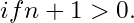
Proof.
Also if  is positive integer.
Result 3. 
For
Result 4.
Proof.

Result 5. Find 
Proof.
Linear Property.
Suppose  and  are Laplace forms of  and  respectively. Then

Where  and  are any constants.
First Shifting Theorem (First Translation)
Proof. Let 
Then, 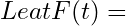


Fact: This theorem can also be restated as:
If  is the Laplace transform of  and a is any real, or complex number, then  is the Laplace transform of). That is to say,
Some examples related with the previous properties and we are going to know how to use these properties to solve a problem
Example. 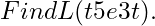
Solution. 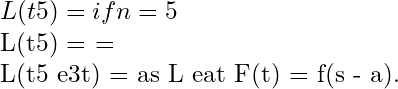

Solution. We know that,
Example. Let’s we are going to prove,
Solution. We know that 

Using the result, , we get
Theorem 4. Second shifting Theorem (Second Translatation).
Statement:- If 
then 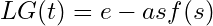
Or 
And 
Example . We are going to find Laplace transform of  where

Solution.  then

Also 
By second shifting theorem, 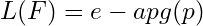

Theorem 5. Change of Scale Property.
If 


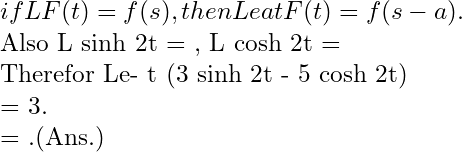
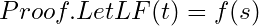
Laplace Transform of Derivatives:
An Alternate form of Theorem 6.
To express the Laplace transform of the function in terms of the Laplace transform of the function 

![In view of this L{F ' (t)} = sg(s) - G(0) = sL {G(t)} - G(0). Taking G(t) = F ' (t), we get L{F ' (t)} = sL {F ' (t)} - F ' (0) = s\[s f(s) - F (0)\] - F ' (0) L{F '' (t)} = s2 f(s) - s F(0) - F ' (0). …………………………(2)](data:image/svg+xml,%3Csvg%20xmlns='http://www.w3.org/2000/svg'%20viewBox='0%200%20774%20123'%3E%3C/svg%3E)![In view of this L{F ' (t)} = sg(s) - G(0) = sL {G(t)} - G(0). Taking G(t) = F ' (t), we get L{F ' (t)} = sL {F ' (t)} - F ' (0) = s\[s f(s) - F (0)\] - F ' (0) L{F '' (t)} = s2 f(s) - s F(0) - F ' (0). …………………………(2)](https://www.mathacademytutoring.com/wp-content/ql-cache/quicklatex.com-1ec27288e3fb547ef8cc531bf9349eed_l3.png)
Generalising the results (1) and (2), we get the required result.
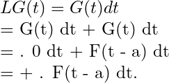
Theorem 7. Laplace Transform of Integral.

 and
 … (1)
We prove that 
From (1) it is clear that
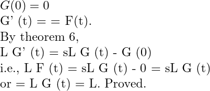

![Example. If , then. Solution. According to, we get = . Dividing by 2, we get . Example on Theorem 7 and Theorem 9: Example. We are going to find Laplace transforms of (a) (b) Solution. If L {F(t) = f(s)\], then L {1 - e- 2t} = L {1} - L {e- 2t} = ∴ L= = = = = = . ⇒ L = . Ans. (b) L(et - cos t) = ⇒ L = = = = = Example. . Solution. We know that = f(s), And L (sin at) = . Hence L (sin t) = . = = = = or, L = cos - 1 s. ∴ L cos - 1 s. Ans.](data:image/svg+xml,%3Csvg%20xmlns='http://www.w3.org/2000/svg'%20viewBox='0%200%20592%20867'%3E%3C/svg%3E)![Example. If , then. Solution. According to, we get = . Dividing by 2, we get . Example on Theorem 7 and Theorem 9: Example. We are going to find Laplace transforms of (a) (b) Solution. If L {F(t) = f(s)\], then L {1 - e- 2t} = L {1} - L {e- 2t} = ∴ L= = = = = = . ⇒ L = . Ans. (b) L(et - cos t) = ⇒ L = = = = = Example. . Solution. We know that = f(s), And L (sin at) = . Hence L (sin t) = . = = = = or, L = cos - 1 s. ∴ L cos - 1 s. Ans.](https://www.mathacademytutoring.com/wp-content/ql-cache/quicklatex.com-77a7d03761348d04d09024c087decb96_l3.png)
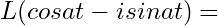
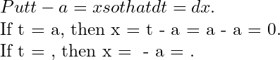
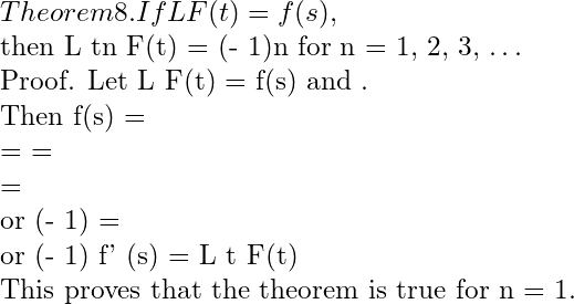
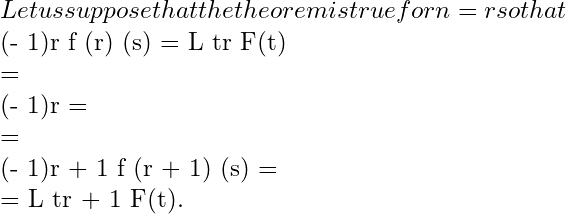
Periodic Functions :
![Theorem 10. Let a function F(t) Be period 𝜔 so that F(t + n𝜔) = F(t) for n = 1, 2, 3, … Then L{F(t)} = Proof. L{F(t)} = = = , where t = x + n𝜔 = \[… F(x + n𝜔) = F(x) for n = 1, 2, 3, …\] = = Hence, L {F(t)} = (… \< 1) Example. If F(t) = t2, 0 \< t \< 2 and F(t + 2) = F(t), then we are going to find L{F(t)}. Solution. Evidently F(t) is a periodic function with period 𝜔 = 2. L {F(t)} = (by Th. 10). = . … (i) Now, = = = = . Now (1) becomes L {F(t)} = .Ans. \<h1\>Standard Rules of Laplace Transform:\</h1\> F (t) L \[F(t)\]= f(p) tn if n + 1 \> 0 1 1/p Cos (at) p/(p2 + a2) Sin (at) a/(p2 + a2) Cosh (at) p/(p2 - a2) Sinh (at) a/(p2 - a2) eat 1/(p - a) J0(at 1/ eat F(t) f (p - a) F(at) F' (t) p f(p) - F(0) tn F(t) (1-)n tan - 1 (a / p) Some problems related with the given chart Problem 1. (a) Find the Laplace transform of t2e - at. Solution. Since L\[tn F(t)\] = (- 1)n F(p) = L\[F(t)\] = L (e - at) = . ∴ L\[ t2e - at\] = (- 1)2 = . Problem 2. We are going to find the Laplace transform of the followings : (i) 2e5t (ii) te2t (iii) sin (at) (iv) L(sin 2t . sin 3t) Solution. We know that L(eat) = … (1) and L\[tn F(t)\] = (- 1)n … (2) L(2e5t) = 2 . L(e5t) = L(te2t) = (Le2t) = = . L(sin at) = L = = = .Ans. L(sin 2t, sin 3t) = \[cos (3t - 2t) - cos (3t + 2t)\] = \[cos t - cos 5t\] = . Ans. Problem 3. Find (i) L\[F(t)\] if F(t) = 1 (ii) L(5t - 2) Solution. (i) = = = .Ans. (ii) Since L(tn) = , L(1) = . Hence L(5t - 2) = 5L(t) - 2L(t) = 5. = .Ans. Problem 4. Find L{cos2 t}, (ii) L{sin2 t}. Solution. We know that L(cos at) = , and L(sin at) = . L(cos2 t) = = = . L(sin2 t) = = = . Problem 5. We are going to show that, L{(1 + te- t)3} = + + + . Solution. We know that L{tn} = if n = 0, 1, 2, 3, …. Then L {tn eat} = . … (1) For L {eat F(t)} = s(s - a) if i{F(t)} = f(s). In view of equation (1), we shall calculate the given transform L{(1 + te- t)3} = L {1 + t3 e-3t + 3te-t + 3t2 e-2t} = L {1} + 3L {te-t} + 3L {t2 e-2t} + 3L {t3 e-3t} = = Proved. Problem 6. Evaluate Solution. Let F(t) = e-t - e-3t. Recall that L {eat} = = L {e-t - e-3t} = ∵ L = , where f(s) = L {F(t)}. This gives, L = = = or = . Putting s = 0, we get = . For log 1 = 0 or = log 3. Ans. log 3. Problem 7. Prove that = . Solution. L cos (at) = ⇒ L = = In view of this = = = = = . Proved. \<h1\>THE LAPLACE TRANSFORM\</h1\> \<h2\>Part II - The Inverse Laplace Transform\</h2\> \<h3\>DEFINITION\</h3\> If the Laplace transform of a function F(t) is f(s) i.e., L {F(t)} = f(s) then F(t) is called an Inverse Laplace transform of f(s). We also write F(t) = L- 1 {f(s)}. L- 1 is called the inverse Laplace transformation operator. Example. L{tn} = . ∴ tn = L- 1 . NULL FUNCTION Let N(t) be a function of t such that Then N(c) is called a null function. Since Laplace transform of all function is zero and hence if L {F(t) = f(s)}, then L {F(t) + N(t)} = f(s). Consequently L- 1 {f(s)} = F(t), L- 1 {f(s)} = F(t) + N(t). This implies that we can have two different functions, with the same Laplace transform. As a result of which the inverse Laplace transform of a function is not unique, if we allow null functions. Hence the inverse Laplace transform of a function is unique if we do not allow null functions which do not appear in case of physical interest. Table of Laplace Transform F (t) f(s) = L {F(t)} 1 tn , n = 0, 1, 2, … eat cos at sin at cosh at sinh at Linear Property : Theorem. If f1(s) and f2(s) are Laplace transform of F1(t) and F2(t) respectively, then L- 1 {c1 f(s) + c2 f(s)} = c1L- 1 { f1 (s)} + c2L- 2 {f2(s)} where c1 and c2 are any constants. Proof. Prove as in theorem 2 of Chapter 1, Part 1, page 10 L {c1 F1(t) + c2 F2(t)} = c1L { F1 (t)} + c2L {F2(t)} = c1 f1 (s) + c2 f2(s) or c1 F1 (t) + c2 F2(t) = L- 1 {c1 f1(s) + c2 f2(s)} or c1 L- 1 {f1(s)} + c2 L- 1 {f2(s)} = L- 1 {c1 f1(s) + c2 f2(s)}. Proved. Example . Find L- 1 . Solution. L- 1 = L- 1 + L- 1 + L- 1 = e2t + 2e- 5t + t3. Example . Find L- 1 . Solution. L- 1 = L- 1 + L- 1 + L- 1 = e2t L- 1 + e- 4t L- 1 + e- 2t L- 1 = e2t cos 5t + e- 4t cos 9t + sin 3t. Ans. Example . Evaluate L- 1 . Solution. Recall that (tn) = . ∴ L = or = L- 1 . Now L- 1 = L- 1 + L- 1 + L- 1 = e4t L- 1 + e2t L- 1 + e- 3t L- 1 = e4t + e2t sin 5t + e- 3t cos 6t. Ans. Example. Prove that L- 1 = (sin t) (sinh t). Solution. L- 1 = L- 1 = p ⟶ p + 1 p ⟶ p - 1 = = \[et sin t - e -t sin t\] = (sin t) (et - e -t) = . Example. Find Solution. = = = = = Ans. Example Find inverse Laplace transform of Solution. = = = = = . Ans. Theorem . Second Shifting Property. If , Then, where G (t) = Proof. = + = + = 0 + = = = = . Thus . ∴ = . Note: This result is also expressible as = or = F(t - a) H(t - a). Where H (t - a) is Heaviside unit step function. Example . Find the inverse Laplace transform of . Solution. say. By second shifting theorem, = = = Example. Evaluate . Solution. Let L {F(t)} = f(s) = . Then, F(t) = = = . By second shifting theorem, = = . Ans. Definition Unit Step Function : The function G(t) such that G(t) = F(t - a) where F(t - a) = 1, t \> a F(t - a) = 0, t \< a is called unit step function and is generally denoted by u(t - a). Theorem. Change of scale property. If f(s) = L{f(s)} denotes the Laplace transform of the function F(t), prove that =, a \> 0. Proof. ∵ , at = x = . For . ∴ = . Proved. Example. If cos t, then Find Solution. cos t. Writing as for s, = . Again writing a = 3, = . Ans. Example. If sin t, then Find . Solution. Here we use F . ∴ . Put a = 4, ⇒ . Ans. Theorem . Inverse Laplace transform of derivatives. If , then Proof. By theorem 8 of chapter 1, Part 1, Page 16. (Prove this) ∴ or . Proved. Example. Evaluate . Solution. Let Then . But or . Ans. Theorem. The Convolution Theorem. If then = . Proof. We have to show that L Let . Aim. L(H) = f(s) g(s) or L(H) = = or L(H) = . … (1) To change the order Limits are : t = 0, t = ∞ and u = 0, u = t. Range of integration is OAB. We want du dt. Draw an elementary strip parallel to T-axis. One end of strip lies on t = u and the other end on t = ∞. For this strip u varies from u = 0 to u = ∞. ∴ = \[Put t - u = y, dt = dy\] = = = = . THE LAPLACE TRANSFORM \<h2\>Part III - The Applications to Differential Equations\</h2\> 1.0. ARTICE Consider the differential equation … (1) Case I. When a, b are constant Here we use Theorem 6, Page 15 namely Taking Laplace transform of (1), . Let . Then . Required solution is obtained by taking the inverse Laplace transform of. Case II. When a, b are functions of t, i.e., (1) is of the type … (2) Here we use Theorem 8, Page 16, i.e., = L {tm x(n) (t)} = . Taking the Laplace transform (2), The required solution is obtained by taking inverse Laplace transform of . WORKED EXAMPLE Problem. Solve by using Laplace transformation : (D2 + 9) y = cos (2t) if y(0) = 1, y = - 1. Solution. Taking Laplace transform, we get p2 - py(0) - y'(0) + 9 = or (p2 + 9) = p + a + where y'(0) = a or = + + or = + + or = + Taking inverse Laplace transform, we get . This ⇒ ∴ . Ans. Problem. Solve , y(0) = 1, y'(0) = 1. Solution. Taking Laplace transform of the equation (2D2 + 5D + 2) y = e- 2t, we get . Putting y(0) = 1 = y'(0), we get ⇒ ⇒ = ⇒ = …(1) = = . (2) But = = . ∴ ∴ ∴ … (3) and ⇒ . … (4) Taking inverse Laplace Transform of (1) and putting values from (2), (3) and (4), we get y = + = . Ans.](data:image/svg+xml,%3Csvg%20xmlns='http://www.w3.org/2000/svg'%20viewBox='0%200%20835%2010076'%3E%3C/svg%3E)![Theorem 10. Let a function F(t) Be period 𝜔 so that F(t + n𝜔) = F(t) for n = 1, 2, 3, … Then L{F(t)} = Proof. L{F(t)} = = = , where t = x + n𝜔 = \[… F(x + n𝜔) = F(x) for n = 1, 2, 3, …\] = = Hence, L {F(t)} = (… \< 1) Example. If F(t) = t2, 0 \< t \< 2 and F(t + 2) = F(t), then we are going to find L{F(t)}. Solution. Evidently F(t) is a periodic function with period 𝜔 = 2. L {F(t)} = (by Th. 10). = . … (i) Now, = = = = . Now (1) becomes L {F(t)} = .Ans. \<h1\>Standard Rules of Laplace Transform:\</h1\> F (t) L \[F(t)\]= f(p) tn if n + 1 \> 0 1 1/p Cos (at) p/(p2 + a2) Sin (at) a/(p2 + a2) Cosh (at) p/(p2 - a2) Sinh (at) a/(p2 - a2) eat 1/(p - a) J0(at 1/ eat F(t) f (p - a) F(at) F' (t) p f(p) - F(0) tn F(t) (1-)n tan - 1 (a / p) Some problems related with the given chart Problem 1. (a) Find the Laplace transform of t2e - at. Solution. Since L\[tn F(t)\] = (- 1)n F(p) = L\[F(t)\] = L (e - at) = . ∴ L\[ t2e - at\] = (- 1)2 = . Problem 2. We are going to find the Laplace transform of the followings : (i) 2e5t (ii) te2t (iii) sin (at) (iv) L(sin 2t . sin 3t) Solution. We know that L(eat) = … (1) and L\[tn F(t)\] = (- 1)n … (2) L(2e5t) = 2 . L(e5t) = L(te2t) = (Le2t) = = . L(sin at) = L = = = .Ans. L(sin 2t, sin 3t) = \[cos (3t - 2t) - cos (3t + 2t)\] = \[cos t - cos 5t\] = . Ans. Problem 3. Find (i) L\[F(t)\] if F(t) = 1 (ii) L(5t - 2) Solution. (i) = = = .Ans. (ii) Since L(tn) = , L(1) = . Hence L(5t - 2) = 5L(t) - 2L(t) = 5. = .Ans. Problem 4. Find L{cos2 t}, (ii) L{sin2 t}. Solution. We know that L(cos at) = , and L(sin at) = . L(cos2 t) = = = . L(sin2 t) = = = . Problem 5. We are going to show that, L{(1 + te- t)3} = + + + . Solution. We know that L{tn} = if n = 0, 1, 2, 3, …. Then L {tn eat} = . … (1) For L {eat F(t)} = s(s - a) if i{F(t)} = f(s). In view of equation (1), we shall calculate the given transform L{(1 + te- t)3} = L {1 + t3 e-3t + 3te-t + 3t2 e-2t} = L {1} + 3L {te-t} + 3L {t2 e-2t} + 3L {t3 e-3t} = = Proved. Problem 6. Evaluate Solution. Let F(t) = e-t - e-3t. Recall that L {eat} = = L {e-t - e-3t} = ∵ L = , where f(s) = L {F(t)}. This gives, L = = = or = . Putting s = 0, we get = . For log 1 = 0 or = log 3. Ans. log 3. Problem 7. Prove that = . Solution. L cos (at) = ⇒ L = = In view of this = = = = = . Proved. \<h1\>THE LAPLACE TRANSFORM\</h1\> \<h2\>Part II - The Inverse Laplace Transform\</h2\> \<h3\>DEFINITION\</h3\> If the Laplace transform of a function F(t) is f(s) i.e., L {F(t)} = f(s) then F(t) is called an Inverse Laplace transform of f(s). We also write F(t) = L- 1 {f(s)}. L- 1 is called the inverse Laplace transformation operator. Example. L{tn} = . ∴ tn = L- 1 . NULL FUNCTION Let N(t) be a function of t such that Then N(c) is called a null function. Since Laplace transform of all function is zero and hence if L {F(t) = f(s)}, then L {F(t) + N(t)} = f(s). Consequently L- 1 {f(s)} = F(t), L- 1 {f(s)} = F(t) + N(t). This implies that we can have two different functions, with the same Laplace transform. As a result of which the inverse Laplace transform of a function is not unique, if we allow null functions. Hence the inverse Laplace transform of a function is unique if we do not allow null functions which do not appear in case of physical interest. Table of Laplace Transform F (t) f(s) = L {F(t)} 1 tn , n = 0, 1, 2, … eat cos at sin at cosh at sinh at Linear Property : Theorem. If f1(s) and f2(s) are Laplace transform of F1(t) and F2(t) respectively, then L- 1 {c1 f(s) + c2 f(s)} = c1L- 1 { f1 (s)} + c2L- 2 {f2(s)} where c1 and c2 are any constants. Proof. Prove as in theorem 2 of Chapter 1, Part 1, page 10 L {c1 F1(t) + c2 F2(t)} = c1L { F1 (t)} + c2L {F2(t)} = c1 f1 (s) + c2 f2(s) or c1 F1 (t) + c2 F2(t) = L- 1 {c1 f1(s) + c2 f2(s)} or c1 L- 1 {f1(s)} + c2 L- 1 {f2(s)} = L- 1 {c1 f1(s) + c2 f2(s)}. Proved. Example . Find L- 1 . Solution. L- 1 = L- 1 + L- 1 + L- 1 = e2t + 2e- 5t + t3. Example . Find L- 1 . Solution. L- 1 = L- 1 + L- 1 + L- 1 = e2t L- 1 + e- 4t L- 1 + e- 2t L- 1 = e2t cos 5t + e- 4t cos 9t + sin 3t. Ans. Example . Evaluate L- 1 . Solution. Recall that (tn) = . ∴ L = or = L- 1 . Now L- 1 = L- 1 + L- 1 + L- 1 = e4t L- 1 + e2t L- 1 + e- 3t L- 1 = e4t + e2t sin 5t + e- 3t cos 6t. Ans. Example. Prove that L- 1 = (sin t) (sinh t). Solution. L- 1 = L- 1 = p ⟶ p + 1 p ⟶ p - 1 = = \[et sin t - e -t sin t\] = (sin t) (et - e -t) = . Example. Find Solution. = = = = = Ans. Example Find inverse Laplace transform of Solution. = = = = = . Ans. Theorem . Second Shifting Property. If , Then, where G (t) = Proof. = + = + = 0 + = = = = . Thus . ∴ = . Note: This result is also expressible as = or = F(t - a) H(t - a). Where H (t - a) is Heaviside unit step function. Example . Find the inverse Laplace transform of . Solution. say. By second shifting theorem, = = = Example. Evaluate . Solution. Let L {F(t)} = f(s) = . Then, F(t) = = = . By second shifting theorem, = = . Ans. Definition Unit Step Function : The function G(t) such that G(t) = F(t - a) where F(t - a) = 1, t \> a F(t - a) = 0, t \< a is called unit step function and is generally denoted by u(t - a). Theorem. Change of scale property. If f(s) = L{f(s)} denotes the Laplace transform of the function F(t), prove that =, a \> 0. Proof. ∵ , at = x = . For . ∴ = . Proved. Example. If cos t, then Find Solution. cos t. Writing as for s, = . Again writing a = 3, = . Ans. Example. If sin t, then Find . Solution. Here we use F . ∴ . Put a = 4, ⇒ . Ans. Theorem . Inverse Laplace transform of derivatives. If , then Proof. By theorem 8 of chapter 1, Part 1, Page 16. (Prove this) ∴ or . Proved. Example. Evaluate . Solution. Let Then . But or . Ans. Theorem. The Convolution Theorem. If then = . Proof. We have to show that L Let . Aim. L(H) = f(s) g(s) or L(H) = = or L(H) = . … (1) To change the order Limits are : t = 0, t = ∞ and u = 0, u = t. Range of integration is OAB. We want du dt. Draw an elementary strip parallel to T-axis. One end of strip lies on t = u and the other end on t = ∞. For this strip u varies from u = 0 to u = ∞. ∴ = \[Put t - u = y, dt = dy\] = = = = . THE LAPLACE TRANSFORM \<h2\>Part III - The Applications to Differential Equations\</h2\> 1.0. ARTICE Consider the differential equation … (1) Case I. When a, b are constant Here we use Theorem 6, Page 15 namely Taking Laplace transform of (1), . Let . Then . Required solution is obtained by taking the inverse Laplace transform of. Case II. When a, b are functions of t, i.e., (1) is of the type … (2) Here we use Theorem 8, Page 16, i.e., = L {tm x(n) (t)} = . Taking the Laplace transform (2), The required solution is obtained by taking inverse Laplace transform of . WORKED EXAMPLE Problem. Solve by using Laplace transformation : (D2 + 9) y = cos (2t) if y(0) = 1, y = - 1. Solution. Taking Laplace transform, we get p2 - py(0) - y'(0) + 9 = or (p2 + 9) = p + a + where y'(0) = a or = + + or = + + or = + Taking inverse Laplace transform, we get . This ⇒ ∴ . Ans. Problem. Solve , y(0) = 1, y'(0) = 1. Solution. Taking Laplace transform of the equation (2D2 + 5D + 2) y = e- 2t, we get . Putting y(0) = 1 = y'(0), we get ⇒ ⇒ = ⇒ = …(1) = = . (2) But = = . ∴ ∴ ∴ … (3) and ⇒ . … (4) Taking inverse Laplace Transform of (1) and putting values from (2), (3) and (4), we get y = + = . Ans.](https://www.mathacademytutoring.com/wp-content/ql-cache/quicklatex.com-229af2f6fa852ffbb5312ca1886079cc_l3.png)
Problem . Using Laplace transform,
solve 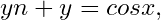 where 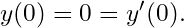
Solution. Taking Laplace transform of given question,
A few worked examples should convince the reader that the Laplace transform furnishes a useful technique for solving liner differential equations. Lastly thanks to all of you and hope you all enjoy this article. We will meet next time with a new article.
Thank You.
References/Bibliography ⟶
This is merely a brief selection. An extensive list is given in reference –
Laplace Transforms and their applications to Differential equations. – N. W. MCLACHLAN
The Laplace Transform: Theory and Applications – Joel L. Schiff
(iii) Ordinary & Partial Differential
(iv) Advanced Calculus – Davis V. Widder
[← PREVIOUS](https://www.mathacademytutoring.com/blog/compact-sets-and-continuous-functions-on-compact-sets) [NEXT →](https://www.mathacademytutoring.com/blog/how-to-integrate-the-function-explained-with-examples)
# Blog Main
#### Categories
- [Math Fun Facts](https://www.mathacademytutoring.com/category/math-fun-facts)
- [Math Learning](https://www.mathacademytutoring.com/category/math-learning)
- [Math Lecture](https://www.mathacademytutoring.com/category/math-lecture)
- [Math Resources](https://www.mathacademytutoring.com/category/math-resources)
- [Students Tips](https://www.mathacademytutoring.com/category/students-tips)
#### Recent Posts
- [How to integrate the function? Explained with examples](https://www.mathacademytutoring.com/blog/how-to-integrate-the-function-explained-with-examples)
- [Laplace Transformation](https://www.mathacademytutoring.com/blog/laplace-transformation)
- [Compact Sets and Continuous Functions on Compact Sets](https://www.mathacademytutoring.com/blog/compact-sets-and-continuous-functions-on-compact-sets)
- [Fourier Series](https://www.mathacademytutoring.com/blog/fourier-series)
- [All The Logarithm Rules You Know and Don’t Know About](https://www.mathacademytutoring.com/blog/all-the-logarithm-rules-you-know-and-dont-know-about)
#### Archives
- [October 2022](https://www.mathacademytutoring.com/blog/2022/10)
- [June 2022](https://www.mathacademytutoring.com/blog/2022/06)
- [February 2022](https://www.mathacademytutoring.com/blog/2022/02)
- [December 2021](https://www.mathacademytutoring.com/blog/2021/12)
- [November 2021](https://www.mathacademytutoring.com/blog/2021/11)
- [October 2021](https://www.mathacademytutoring.com/blog/2021/10)
- [September 2021](https://www.mathacademytutoring.com/blog/2021/09)
- [August 2021](https://www.mathacademytutoring.com/blog/2021/08)
- [June 2021](https://www.mathacademytutoring.com/blog/2021/06)
- [May 2021](https://www.mathacademytutoring.com/blog/2021/05)
- [April 2021](https://www.mathacademytutoring.com/blog/2021/04)
- [February 2021](https://www.mathacademytutoring.com/blog/2021/02)
- [January 2021](https://www.mathacademytutoring.com/blog/2021/01)
#### Categories
- [Math Fun Facts](https://www.mathacademytutoring.com/category/math-fun-facts)
- [Math Learning](https://www.mathacademytutoring.com/category/math-learning)
- [Math Lecture](https://www.mathacademytutoring.com/category/math-lecture)
- [Math Resources](https://www.mathacademytutoring.com/category/math-resources)
- [Students Tips](https://www.mathacademytutoring.com/category/students-tips)
#### Meta
- [Log in](https://www.mathacademytutoring.com/wp-login.php)
- [Entries feed](https://www.mathacademytutoring.com/feed)
- [Comments feed](https://www.mathacademytutoring.com/comments/feed)
- [WordPress.org](https://wordpress.org/)
Featured Bundles
- [Basic School Math](https://www.mathacademytutoring.com/tutoring/online-tutoring/basic-school-math)
- [College Math](https://www.mathacademytutoring.com/tutoring/online-tutoring/college-math)
- [Graduate Math](https://www.mathacademytutoring.com/tutoring/online-tutoring/graduate-math)
- [Data Science Bundle](https://www.mathacademytutoring.com/tutoring/online-tutoring/data-science-bundle)
- [Python Tutoring Online](https://www.mathacademytutoring.com/online-python-tutoring-for-data-science)
Your first session is only \$20, [Sign up here ](https://www.mathacademytutoring.com/cart/?add-to-cart=10047)


Get Online One-on-One Tutoring with the Math Pros; Basic High School, College, Graduate, Test Prep & beyond.
[](mailto:info@mathacademytutoring.com)
[\+1 (718) 864-9087](<tel:+1 (718) 864-9087>)
[](mailto:info@mathacademytutoring.com)
[info@mathacademytutoring.com](mailto:info@mathacademytutoring.com)
Page Links
- [Courses](https://www.mathacademytutoring.com/courses)
- [For Schools](https://www.mathacademytutoring.com/for-schools)
- [Testimonials](https://www.mathacademytutoring.com/testimonials)
- [Our Team](https://www.mathacademytutoring.com/our-team)
- [Tutor With Us](https://www.mathacademytutoring.com/tutor-with-us)
- [FAQ – Help](https://www.mathacademytutoring.com/faq-help)
- [Refund Policy](https://www.mathacademytutoring.com/refund-policy)
- [Privacy & Terms](https://www.mathacademytutoring.com/privacy-terms)
- [Blog](https://www.mathacademytutoring.com/blog)
- [Contact](https://www.mathacademytutoring.com/contact)
Top Courses
- [Basic School Math](https://www.mathacademytutoring.com/tutoring/online-tutoring/basic-school-math)
- [College Math](https://www.mathacademytutoring.com/tutoring/online-tutoring/college-math)
- [Graduate Math](https://www.mathacademytutoring.com/tutoring/online-tutoring/graduate-math)
- [Data Science Bundle](https://www.mathacademytutoring.com/tutoring/online-tutoring/data-science-bundle)
- [Python Tutoring Online](https://www.mathacademytutoring.com/online-python-tutoring-for-data-science)
Connect With Us
[](https://www.linkedin.com/company/math-and-science-academy-msa/) [](https://www.facebook.com/mathacademytutoring/) [](https://www.instagram.com/math_guideline/)
We Accept
   
[Privacy Policy](https://www.mathacademytutoring.com/privacy-terms) \| [Refund Policy](https://www.mathacademytutoring.com/refund-policy) \| [Sitemap](https://www.mathacademytutoring.com/blog/laplace-transformation)
Copyright © 2025 Math Academy. All Rights Reserved.
Share This
- [Facebook](http://www.facebook.com/sharer.php?u=https%3A%2F%2Fwww.mathacademytutoring.com%2Fblog%2Flaplace-transformation&t=Laplace%20Transformation)
- [LinkedIn](http://www.linkedin.com/shareArticle?mini=true&url=https%3A%2F%2Fwww.mathacademytutoring.com%2Fblog%2Flaplace-transformation&title=Laplace%20Transformation)
- [Twitter](http://twitter.com/share?text=Laplace%20Transformation&url=https%3A%2F%2Fwww.mathacademytutoring.com%2Fblog%2Flaplace-transformation)
- [Gmail](https://mail.google.com/mail/u/0/?view=cm&fs=1&su=Laplace%20Transformation&body=https%3A%2F%2Fwww.mathacademytutoring.com%2Fblog%2Flaplace-transformation&ui=2&tf=1) |
| Readable Markdown | Table of Contents
- [HISTORY](https://www.mathacademytutoring.com/blog/laplace-transformation#history)
- [INTRODUCTION](https://www.mathacademytutoring.com/blog/laplace-transformation#introduction)
- [PIECE-WISE OR SECTIONAL CONTINUITY](https://www.mathacademytutoring.com/blog/laplace-transformation#piece-wise-or-sectional-continuity)
- [FUNCTION OF EXPONENTIAL ORDER](https://www.mathacademytutoring.com/blog/laplace-transformation#function-of-exponential-order)
- [DEFINITION OF THE TRANSFORM CONCEPT](https://www.mathacademytutoring.com/blog/laplace-transformation#definition-of-the-transform-concept)
- [DEFINITION. LAPLACE TRANSFORM](https://www.mathacademytutoring.com/blog/laplace-transformation#definition-laplace-transform)
- [LAPLACE TRANSFORMS OF STANDARD FUNCTION](https://www.mathacademytutoring.com/blog/laplace-transformation#laplace-transforms-of-standard-function)
## HISTORY
Integral transformation data back to the Work of Leonard Euler (1763 & 1769), who considered them essentially in the form of the inverse Laplace transform in solving second-order, linear ordinary differential equations. Even Laplace, in his great work, “Theorie Analytique Des Probabilities”(1812), credits Euler with introducing integral transforms. It is Spitzer (1878) who attached the name of Laplace to the expression

Employed by Euler. In this form, it is substituted into the differential equation where  is the unknown function of the variable .
In the late 19th century, the Laplace transform was extended to his complex form by Poincare and Pincherle, Redis covered by Petzval, and extended to two variables by Picard, with the further investigation conducted by Abel and many others.
The first application of the modern Laplace transformations equations arose of Batemer (1910), who was working on radioactive decay

By setting

and obtaining the transformed equation. Bernstein (1920) used the expression

called it the Laplace transformation, in his work on theta functions. The modern approach was given particular impetus by Doetsch in the 1920s and 30s; he applied the Laplace transform to differential, integral, and integro-differential equations. This body of work culminated in his foundational 1937 text, “Theorie and Anwendungender Laplace Transformation.”
No account of the Laplace transformation would be complete without mention of the work of Oliver Heaviside, who produced a vast body of what is termed the “Operational Calculus”. The material is scattered throughout his three volumes, Electromagnetic Theory (1894, 1899, 1912), and bears many similarities to the Laplace transform method. Although Heaviside’s calculus was not the theory of Laplace Transformation, he did find favour with electrical engineers as a useful technique for solving their problems. Considerable research went into trying to make the Heaviside calculus rigorous and connecting it with the Laplace transform. One such effort was that of Bromwich, who, among others, discovered the Inverse Laplace Transformation\!
Where lying to the right of all singularities of the function .
## INTRODUCTION
In this article, we shall consider theoretic aspects of the Laplace transform, reserving for the application of the subject to the solution of linear differential equations. This transformation is defined by the equation;
## PIECE-WISE OR SECTIONAL CONTINUITY
A function is called sectionally continuous or piece-wise continuous in any interval if it is continuous and has finite left and right-hand limits in every subinterval as shown in the graph of the function
## FUNCTION OF EXPONENTIAL ORDER
A function is said to be of exponential order as 
if
i.e., if given a positive integer, there exists a real number 
Or
Briefly, we say that  is of exponential order.
Sometimes we write,
For example. is of exponential order as being any positive integer.
So we are going to do L’Hospital Rule where we differentiate numerator and denominator individually,
hence,
(by L. Hospital’s rule)
\=
Since.
Hence we can say that is an exponential order as.
Another example. is not of exponential order as 
Taking, 
Therefore, 
 is not of exponential order
## DEFINITION OF THE TRANSFORM CONCEPT
An improper integral of the form is called Integral Transform of  if it is convergent. Sometimes it is denoted by or Thus
The function  appearing in the integrand is called Kernel of the transform. Here’s a parameter and is independent of  may be real or complex number.
If we take
Then  becomes
This transform is known as Laplace transform.
Some examples of well-known transformations
Hankel Transform of  is
Mellin Transform of  is
Fourier transform of  is
## DEFINITION. LAPLACE TRANSFORM
Suppose is a real valued function defined over the interval 
The Laplace Transform of, denoted by, is defined as
We also write
Here L is called Laplace transformation operator. The parameter s is a real or complex number. In general, the parameter  is taken to be a real positive number. Sometimes we use symbol  for parameter .
The Laplace transform is said to exist if the integral (1) is convergent for some value of .
The operation of multiplying by  and integrating from  is called Laplace Transformation.
Now we are going to see the existence of Laplace transformation on a function
Existence Theorem of Laplace Transform.
Statement: – If is a function of class , then Laplace transform of  exists.
Or,
Suppose is piece-wise continuous in every finite interval and is of exponential order an as. Then exists , i.e., Laplace transform exists.
Proof. Let  be piece-wise continuous in every finite interval and of exponential order as 
To show that ![f(s) = L \[F(t)\] exists s \> a.](https://www.mathacademytutoring.com/wp-content/ql-cache/quicklatex.com-f62affc1953bff7c2154387381748af9_l3.png)
Let  Then
Continuity of  in the finite interval  implies that
exists. It remains to show that
exists  is of exponential order a  implies
is finite, i.e., given a number , there exists a real number 


i.e.,
can be made as small as we please choosing  sufficiently large. Hence exists 
Fact: The condition given in this part is sufficient for the existence of, but are not the necessary conditions.
## LAPLACE TRANSFORMS OF STANDARD FUNCTION
Result 1.
Proof.
Result 2. 
Proof.
Also if  is positive integer.
Result 3. 
For
Result 4.
Proof.


Result 5. Find 
Proof.


Linear Property.
Suppose  and  are Laplace forms of  and  respectively. Then

Where  and  are any constants.
First Shifting Theorem (First Translation)
Proof. Let 
Then, 


Fact: This theorem can also be restated as:
If  is the Laplace transform of  and a is any real, or complex number, then  is the Laplace transform of). That is to say,
Some examples related with the previous properties and we are going to know how to use these properties to solve a problem
Example. 
Solution. 

Solution. We know that,

Example. Let’s we are going to prove,
Solution. We know that 


Using the result, , we get
Theorem 4. Second shifting Theorem (Second Translatation).
Statement:- If 
then 
Or 
And 


Example . We are going to find Laplace transform of  where

Solution.  then

Also 
By second shifting theorem, 

Theorem 5. Change of Scale Property.
If 


Laplace Transform of Derivatives:

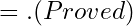
An Alternate form of Theorem 6.
To express the Laplace transform of the function in terms of the Laplace transform of the function 


![In view of this L{F ' (t)} = sg(s) - G(0) = sL {G(t)} - G(0). Taking G(t) = F ' (t), we get L{F ' (t)} = sL {F ' (t)} - F ' (0) = s\[s f(s) - F (0)\] - F ' (0) L{F '' (t)} = s2 f(s) - s F(0) - F ' (0). …………………………(2)](https://www.mathacademytutoring.com/wp-content/ql-cache/quicklatex.com-1ec27288e3fb547ef8cc531bf9349eed_l3.png)
Generalising the results (1) and (2), we get the required result.
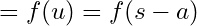
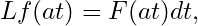
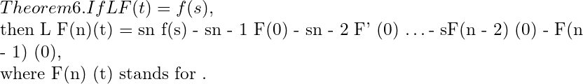
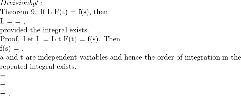
Theorem 7. Laplace Transform of Integral.

 and
 … (1)
We prove that 
From (1) it is clear that


![Example. If , then. Solution. According to, we get = . Dividing by 2, we get . Example on Theorem 7 and Theorem 9: Example. We are going to find Laplace transforms of (a) (b) Solution. If L {F(t) = f(s)\], then L {1 - e- 2t} = L {1} - L {e- 2t} = ∴ L= = = = = = . ⇒ L = . Ans. (b) L(et - cos t) = ⇒ L = = = = = Example. . Solution. We know that = f(s), And L (sin at) = . Hence L (sin t) = . = = = = or, L = cos - 1 s. ∴ L cos - 1 s. Ans.](https://www.mathacademytutoring.com/wp-content/ql-cache/quicklatex.com-77a7d03761348d04d09024c087decb96_l3.png)
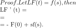
Periodic Functions :
![Theorem 10. Let a function F(t) Be period 𝜔 so that F(t + n𝜔) = F(t) for n = 1, 2, 3, … Then L{F(t)} = Proof. L{F(t)} = = = , where t = x + n𝜔 = \[… F(x + n𝜔) = F(x) for n = 1, 2, 3, …\] = = Hence, L {F(t)} = (… \< 1) Example. If F(t) = t2, 0 \< t \< 2 and F(t + 2) = F(t), then we are going to find L{F(t)}. Solution. Evidently F(t) is a periodic function with period 𝜔 = 2. L {F(t)} = (by Th. 10). = . … (i) Now, = = = = . Now (1) becomes L {F(t)} = .Ans. \<h1\>Standard Rules of Laplace Transform:\</h1\> F (t) L \[F(t)\]= f(p) tn if n + 1 \> 0 1 1/p Cos (at) p/(p2 + a2) Sin (at) a/(p2 + a2) Cosh (at) p/(p2 - a2) Sinh (at) a/(p2 - a2) eat 1/(p - a) J0(at 1/ eat F(t) f (p - a) F(at) F' (t) p f(p) - F(0) tn F(t) (1-)n tan - 1 (a / p) Some problems related with the given chart Problem 1. (a) Find the Laplace transform of t2e - at. Solution. Since L\[tn F(t)\] = (- 1)n F(p) = L\[F(t)\] = L (e - at) = . ∴ L\[ t2e - at\] = (- 1)2 = . Problem 2. We are going to find the Laplace transform of the followings : (i) 2e5t (ii) te2t (iii) sin (at) (iv) L(sin 2t . sin 3t) Solution. We know that L(eat) = … (1) and L\[tn F(t)\] = (- 1)n … (2) L(2e5t) = 2 . L(e5t) = L(te2t) = (Le2t) = = . L(sin at) = L = = = .Ans. L(sin 2t, sin 3t) = \[cos (3t - 2t) - cos (3t + 2t)\] = \[cos t - cos 5t\] = . Ans. Problem 3. Find (i) L\[F(t)\] if F(t) = 1 (ii) L(5t - 2) Solution. (i) = = = .Ans. (ii) Since L(tn) = , L(1) = . Hence L(5t - 2) = 5L(t) - 2L(t) = 5. = .Ans. Problem 4. Find L{cos2 t}, (ii) L{sin2 t}. Solution. We know that L(cos at) = , and L(sin at) = . L(cos2 t) = = = . L(sin2 t) = = = . Problem 5. We are going to show that, L{(1 + te- t)3} = + + + . Solution. We know that L{tn} = if n = 0, 1, 2, 3, …. Then L {tn eat} = . … (1) For L {eat F(t)} = s(s - a) if i{F(t)} = f(s). In view of equation (1), we shall calculate the given transform L{(1 + te- t)3} = L {1 + t3 e-3t + 3te-t + 3t2 e-2t} = L {1} + 3L {te-t} + 3L {t2 e-2t} + 3L {t3 e-3t} = = Proved. Problem 6. Evaluate Solution. Let F(t) = e-t - e-3t. Recall that L {eat} = = L {e-t - e-3t} = ∵ L = , where f(s) = L {F(t)}. This gives, L = = = or = . Putting s = 0, we get = . For log 1 = 0 or = log 3. Ans. log 3. Problem 7. Prove that = . Solution. L cos (at) = ⇒ L = = In view of this = = = = = . Proved. \<h1\>THE LAPLACE TRANSFORM\</h1\> \<h2\>Part II - The Inverse Laplace Transform\</h2\> \<h3\>DEFINITION\</h3\> If the Laplace transform of a function F(t) is f(s) i.e., L {F(t)} = f(s) then F(t) is called an Inverse Laplace transform of f(s). We also write F(t) = L- 1 {f(s)}. L- 1 is called the inverse Laplace transformation operator. Example. L{tn} = . ∴ tn = L- 1 . NULL FUNCTION Let N(t) be a function of t such that Then N(c) is called a null function. Since Laplace transform of all function is zero and hence if L {F(t) = f(s)}, then L {F(t) + N(t)} = f(s). Consequently L- 1 {f(s)} = F(t), L- 1 {f(s)} = F(t) + N(t). This implies that we can have two different functions, with the same Laplace transform. As a result of which the inverse Laplace transform of a function is not unique, if we allow null functions. Hence the inverse Laplace transform of a function is unique if we do not allow null functions which do not appear in case of physical interest. Table of Laplace Transform F (t) f(s) = L {F(t)} 1 tn , n = 0, 1, 2, … eat cos at sin at cosh at sinh at Linear Property : Theorem. If f1(s) and f2(s) are Laplace transform of F1(t) and F2(t) respectively, then L- 1 {c1 f(s) + c2 f(s)} = c1L- 1 { f1 (s)} + c2L- 2 {f2(s)} where c1 and c2 are any constants. Proof. Prove as in theorem 2 of Chapter 1, Part 1, page 10 L {c1 F1(t) + c2 F2(t)} = c1L { F1 (t)} + c2L {F2(t)} = c1 f1 (s) + c2 f2(s) or c1 F1 (t) + c2 F2(t) = L- 1 {c1 f1(s) + c2 f2(s)} or c1 L- 1 {f1(s)} + c2 L- 1 {f2(s)} = L- 1 {c1 f1(s) + c2 f2(s)}. Proved. Example . Find L- 1 . Solution. L- 1 = L- 1 + L- 1 + L- 1 = e2t + 2e- 5t + t3. Example . Find L- 1 . Solution. L- 1 = L- 1 + L- 1 + L- 1 = e2t L- 1 + e- 4t L- 1 + e- 2t L- 1 = e2t cos 5t + e- 4t cos 9t + sin 3t. Ans. Example . Evaluate L- 1 . Solution. Recall that (tn) = . ∴ L = or = L- 1 . Now L- 1 = L- 1 + L- 1 + L- 1 = e4t L- 1 + e2t L- 1 + e- 3t L- 1 = e4t + e2t sin 5t + e- 3t cos 6t. Ans. Example. Prove that L- 1 = (sin t) (sinh t). Solution. L- 1 = L- 1 = p ⟶ p + 1 p ⟶ p - 1 = = \[et sin t - e -t sin t\] = (sin t) (et - e -t) = . Example. Find Solution. = = = = = Ans. Example Find inverse Laplace transform of Solution. = = = = = . Ans. Theorem . Second Shifting Property. If , Then, where G (t) = Proof. = + = + = 0 + = = = = . Thus . ∴ = . Note: This result is also expressible as = or = F(t - a) H(t - a). Where H (t - a) is Heaviside unit step function. Example . Find the inverse Laplace transform of . Solution. say. By second shifting theorem, = = = Example. Evaluate . Solution. Let L {F(t)} = f(s) = . Then, F(t) = = = . By second shifting theorem, = = . Ans. Definition Unit Step Function : The function G(t) such that G(t) = F(t - a) where F(t - a) = 1, t \> a F(t - a) = 0, t \< a is called unit step function and is generally denoted by u(t - a). Theorem. Change of scale property. If f(s) = L{f(s)} denotes the Laplace transform of the function F(t), prove that =, a \> 0. Proof. ∵ , at = x = . For . ∴ = . Proved. Example. If cos t, then Find Solution. cos t. Writing as for s, = . Again writing a = 3, = . Ans. Example. If sin t, then Find . Solution. Here we use F . ∴ . Put a = 4, ⇒ . Ans. Theorem . Inverse Laplace transform of derivatives. If , then Proof. By theorem 8 of chapter 1, Part 1, Page 16. (Prove this) ∴ or . Proved. Example. Evaluate . Solution. Let Then . But or . Ans. Theorem. The Convolution Theorem. If then = . Proof. We have to show that L Let . Aim. L(H) = f(s) g(s) or L(H) = = or L(H) = . … (1) To change the order Limits are : t = 0, t = ∞ and u = 0, u = t. Range of integration is OAB. We want du dt. Draw an elementary strip parallel to T-axis. One end of strip lies on t = u and the other end on t = ∞. For this strip u varies from u = 0 to u = ∞. ∴ = \[Put t - u = y, dt = dy\] = = = = . THE LAPLACE TRANSFORM \<h2\>Part III - The Applications to Differential Equations\</h2\> 1.0. ARTICE Consider the differential equation … (1) Case I. When a, b are constant Here we use Theorem 6, Page 15 namely Taking Laplace transform of (1), . Let . Then . Required solution is obtained by taking the inverse Laplace transform of. Case II. When a, b are functions of t, i.e., (1) is of the type … (2) Here we use Theorem 8, Page 16, i.e., = L {tm x(n) (t)} = . Taking the Laplace transform (2), The required solution is obtained by taking inverse Laplace transform of . WORKED EXAMPLE Problem. Solve by using Laplace transformation : (D2 + 9) y = cos (2t) if y(0) = 1, y = - 1. Solution. Taking Laplace transform, we get p2 - py(0) - y'(0) + 9 = or (p2 + 9) = p + a + where y'(0) = a or = + + or = + + or = + Taking inverse Laplace transform, we get . This ⇒ ∴ . Ans. Problem. Solve , y(0) = 1, y'(0) = 1. Solution. Taking Laplace transform of the equation (2D2 + 5D + 2) y = e- 2t, we get . Putting y(0) = 1 = y'(0), we get ⇒ ⇒ = ⇒ = …(1) = = . (2) But = = . ∴ ∴ ∴ … (3) and ⇒ . … (4) Taking inverse Laplace Transform of (1) and putting values from (2), (3) and (4), we get y = + = . Ans.](https://www.mathacademytutoring.com/wp-content/ql-cache/quicklatex.com-229af2f6fa852ffbb5312ca1886079cc_l3.png)
Problem . Using Laplace transform,
solve  where 
Solution. Taking Laplace transform of given question,

A few worked examples should convince the reader that the Laplace transform furnishes a useful technique for solving liner differential equations. Lastly thanks to all of you and hope you all enjoy this article. We will meet next time with a new article.
Thank You.
References/Bibliography ⟶
This is merely a brief selection. An extensive list is given in reference –
Laplace Transforms and their applications to Differential equations. – N. W. MCLACHLAN
The Laplace Transform: Theory and Applications – Joel L. Schiff
(iii) Ordinary & Partial Differential
(iv) Advanced Calculus – Davis V. Widder |
| Shard | 10 (laksa) |
| Root Hash | 17582869072185195810 |
| Unparsed URL | com,mathacademytutoring!www,/blog/laplace-transformation s443 |