ℹ️ Skipped - page is already crawled
| Filter | Status | Condition | Details |
|---|---|---|---|
| HTTP status | PASS | download_http_code = 200 | HTTP 200 |
| Age cutoff | PASS | download_stamp > now() - 6 MONTH | 0.8 months ago |
| History drop | PASS | isNull(history_drop_reason) | No drop reason |
| Spam/ban | PASS | fh_dont_index != 1 AND ml_spam_score = 0 | ml_spam_score=0 |
| Canonical | PASS | meta_canonical IS NULL OR = '' OR = src_unparsed | Not set |
| Property | Value | |||||||||||||||
|---|---|---|---|---|---|---|---|---|---|---|---|---|---|---|---|---|
| URL | https://www.itl.nist.gov/div898/handbook/pmc/section4/pmc431.htm | |||||||||||||||
| Last Crawled | 2026-03-31 11:31:59 (24 days ago) | |||||||||||||||
| First Indexed | 2018-04-04 10:44:37 (8 years ago) | |||||||||||||||
| HTTP Status Code | 200 | |||||||||||||||
| Content | ||||||||||||||||
| Meta Title | 6.4.3.1. Single Exponential Smoothing | |||||||||||||||
| Meta Description | null | |||||||||||||||
| Meta Canonical | null | |||||||||||||||
| Boilerpipe Text | 6.
Process or Product Monitoring and Control
6.4.
Introduction to Time Series Analysis
6.4.3.
What is Exponential Smoothing?
Single Exponential Smoothing
Exponential smoothing weights past observations with exponentially
decreasing weights to forecast future values
This smoothing scheme begins by setting
S
2
to
y
1
,
where
S
i
stands for smoothed observation or EWMA, and
y
stands for the original observation.
The subscripts refer to the time periods,
1
,
2
,
…
,
n
.
For the third period,
S
3
=
α
y
2
+
(
1
−
α
)
S
2
;
and so on. There is no
S
1
;
the smoothed series starts with the smoothed version of the second observation.
For any time period
t
,
the smoothed value
S
t
is found by computing
S
t
=
α
y
t
−
1
+
(
1
−
α
)
S
t
−
1
0
<
α
≤
1
t
≥
3
.
This is the
basic equation of exponential smoothing
and the
constant or parameter
α
is called the
smoothing constant
.
Note
: There is an alternative approach to exponential smoothing
that replaces
y
t
−
1
in the basic equation with
y
t
,
the current observation. That formulation,
due to Roberts (1959), is described in the section on
EWMA control charts
.
The formulation here follows Hunter (1986).
Setting the first EWMA
The first forecast is very important
The initial EWMA plays an important role in computing all the
subsequent EWMAs. Setting
S
2
to
y
1
is one method of initialization. Another way is to set it to the target of the process.
Still another possibility would be to average the first four or five
observations.
It can also be shown that the smaller the value of
α
,
the more important is the selection of the initial EWMA. The user would
be wise to try a few methods, (assuming that the software has them
available) before finalizing the settings.
Why is it called "Exponential"?
Expand basic equation
Let us expand the basic equation by first substituting for
S
t
−
1
in the basic equation to obtain
S
t
=
α
y
t
−
1
+
(
1
−
α
)
[
α
y
t
−
2
+
(
1
−
α
)
S
t
−
2
]
=
α
y
t
−
1
+
α
(
1
−
α
)
y
t
−
2
+
(
1
−
α
)
2
S
t
−
2
.
Summation formula for basic equation
By substituting for
S
t
−
2
,
then for
S
t
−
3
,
and so forth, until we reach
S
2
(which is just
y
1
),
it can be shown that the expanding equation can be written as:
S
t
=
α
∑
i
=
1
t
−
2
(
1
−
α
)
i
−
1
y
t
−
i
+
(
1
−
α
)
t
−
2
S
2
,
t
≥
2
.
Expanded equation for
S
5
For example, the expanded equation for the smoothed value
S
5
is:
S
5
=
α
[
(
1
−
α
)
0
y
5
−
1
+
(
1
−
α
)
1
y
5
−
2
+
(
1
−
α
)
2
y
5
−
3
]
+
(
1
−
α
)
3
S
2
. | |||||||||||||||
| Markdown | 
| | |
|---|---|
| | |
| 6\.4.3.1. | Single Exponential Smoothing |
| *Exponential smoothing weights past observations with exponentially decreasing weights to forecast future values* | This smoothing scheme begins by setting S 2 to y 1, where S i stands for smoothed observation or EWMA, and y stands for the original observation. The subscripts refer to the time periods, 1 , 2 , … , n. For the third period, S 3 \= α y 2 \+ ( 1 − α ) S 2; and so on. There is no S 1; the smoothed series starts with the smoothed version of the second observation. For any time period t, the smoothed value S t is found by computing S t \= α y t − 1 \+ ( 1 − α ) S t − 1 0 \< α ≤ 1 t ≥ 3 . This is the *basic equation of exponential smoothing* and the constant or parameter α is called the *smoothing constant*.**Note**: There is an alternative approach to exponential smoothing that replaces y t − 1 in the basic equation with y t, the current observation. That formulation, due to Roberts (1959), is described in the section on [EWMA control charts](https://www.itl.nist.gov/div898/handbook/pmc/section3/pmc324.htm). The formulation here follows Hunter (1986). |
| | **Setting the first EWMA** |
| *The first forecast is very important* | The initial EWMA plays an important role in computing all the subsequent EWMAs. Setting S 2 to y 1 is one method of initialization. Another way is to set it to the target of the process. Still another possibility would be to average the first four or five observations.It can also be shown that the smaller the value of α, the more important is the selection of the initial EWMA. The user would be wise to try a few methods, (assuming that the software has them available) before finalizing the settings. |
| | **Why is it called "Exponential"?** |
| *Expand basic equation* | Let us expand the basic equation by first substituting for S t − 1 in the basic equation to obtain S t \= α y t − 1 \+ ( 1 − α ) \[ α y t − 2 \+ ( 1 − α ) S t − 2 \] \= α y t − 1 \+ α ( 1 − α ) y t − 2 \+ ( 1 − α ) 2 S t − 2 . |
| *Summation formula for basic equation* | By substituting for S t − 2, then for S t − 3, and so forth, until we reach S 2 (which is just y 1), it can be shown that the expanding equation can be written as: S t \= α ∑ i \= 1 t − 2 ( 1 − α ) i − 1 y t − i \+ ( 1 − α ) t − 2 S 2 , t ≥ 2 . |
| *Expanded equation for S 5* | For example, the expanded equation for the smoothed value S 5 is: S 5 \= α \[ ( 1 − α ) 0 y 5 − 1 \+ ( 1 − α ) 1 y 5 − 2 \+ ( 1 − α ) 2 y 5 − 3 \] \+ ( 1 − α ) 3 S 2 . |
| | | | | |
|---|---|---|---|---|
| *Illustrates exponential behavior* | This illustrates the exponential behavior. The weights, α ( 1 − α ) t decrease geometrically, and their sum is unity as shown below, using a property of geometric series: α ∑ i \= 0 t − 1 ( 1 − α ) i \= α \[ 1 − ( 1 − α ) t 1 − ( 1 − α ) \] \= 1 − ( 1 − α ) t . From the last formula we can see that the summation term shows that the contribution to the smoothed value S t becomes less at each consecutive time period. | | | |
| *Example for α \= 0\.3* | | | | |
| | Value | weight | | |
| last | y 1 | 0\.2100 | | |
| | y 2 | 0\.1470 | | |
| | y 3 | 0\.1029 | | |
| | y 4 | 0\.0720 | | |
| | **What is the "best" value for α?** | | | |
| *How do you choose the weight parameter?* | | | | |
| | | | | |
| α | ( 1 − α ) | ( 1 − α ) 2 | ( 1 − α ) 3 | ( 1 − α ) 4 |
| 0\.9 | 0\.1 | 0\.01 | 0\.001 | 0\.0001 |
| 0\.5 | 0\.5 | 0\.25 | 0\.125 | 0\.0625 |
| 0\.1 | 0\.9 | 0\.81 | 0\.729 | 0\.6561 |
| *Example* | | | | |
| Time | y t | S ( α \= 0\.1 ) | Error | Error squared |
| 1 | 71 | | | |
| 2 | 70 | 71 | \-1.00 | 1\.00 |
| 3 | 69 | 70\.9 | \-1.90 | 3\.61 |
| 4 | 68 | 70\.71 | \-2.71 | 7\.34 |
| 5 | 64 | 70\.44 | \-6.44 | 41\.47 |
| 6 | 65 | 69\.80 | \-4.80 | 23\.04 |
| 7 | 72 | 69\.32 | 2\.68 | 7\.18 |
| 8 | 78 | 69\.58 | 8\.42 | 70\.90 |
| 9 | 75 | 70\.43 | 4\.57 | 20\.88 |
| 10 | 75 | 70\.88 | 4\.12 | 16\.97 |
| 11 | 75 | 71\.29 | 3\.71 | 13\.76 |
| 12 | 70 | 71\.67 | \-1.67 | 2\.79 |
| *Calculate for different values of α* | The MSE was again calculated for α \= 0\.5 and turned out to be 16.29, so in this case we would prefer an α of 0.5. Can we do better? We could apply the proven trial-and-error method. This is an iterative procedure beginning with a range of α between 0.1 and 0.9. We determine the best initial choice for α and then search between α − Δ and α \+ Δ. We could repeat this perhaps one more time to find the best α to 3 decimal places. | | | |
| *Nonlinear optimizers can be used* | But there are better search methods, such as the Marquardt procedure. This is a nonlinear optimizer that minimizes the sum of squares of residuals. In general, most well designed statistical software programs should be able to find the value of α that minimizes the MSE. | | | |
| *Sample plot showing smoothed data for 2 values of α* | 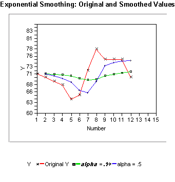 | | | |

- [Site Privacy](https://www.nist.gov/privacy-policy)
- [Accessibility](https://www.nist.gov/oism/accessibility)
- [Privacy Program](https://www.nist.gov/privacy)
- [Copyrights](https://www.nist.gov/oism/copyrights)
- [Vulnerability Disclosure](https://www.commerce.gov/vulnerability-disclosure-policy)
- [No Fear Act Policy](https://www.nist.gov/no-fear-act-policy)
- [FOIA](https://www.nist.gov/foia)
- [Environmental Policy](https://www.nist.gov/environmental-policy-statement)
- [Scientific Integrity](https://www.nist.gov/summary-report-scientific-integrity)
- [Information Quality Standards](https://www.nist.gov/nist-information-quality-standards)
- [Commerce.gov](https://www.commerce.gov/)
- [Science.gov](https://www.science.gov/)
- [USA.gov](https://www.usa.gov/)
- [Vote.gov](https://vote.gov/)
[](https://www.nist.gov/ "National Institute of Standards and Technology") | |||||||||||||||
| Readable Markdown | null | |||||||||||||||
| ML Classification | ||||||||||||||||
| ML Categories |
Raw JSON{
"/Science": 803,
"/Science/Mathematics": 355,
"/Science/Mathematics/Statistics": 320,
"/Computers_and_Electronics": 198,
"/Computers_and_Electronics/Software": 156
} | |||||||||||||||
| ML Page Types |
Raw JSON{
"/Article": 807,
"/Article/Tutorial_or_Guide": 765
} | |||||||||||||||
| ML Intent Types |
Raw JSON{
"Informational": 999
} | |||||||||||||||
| Content Metadata | ||||||||||||||||
| Language | null | |||||||||||||||
| Author | null | |||||||||||||||
| Publish Time | not set | |||||||||||||||
| Original Publish Time | 2018-04-04 10:44:37 (8 years ago) | |||||||||||||||
| Republished | No | |||||||||||||||
| Word Count (Total) | 1,142 | |||||||||||||||
| Word Count (Content) | 569 | |||||||||||||||
| Links | ||||||||||||||||
| External Links | 5 | |||||||||||||||
| Internal Links | 27 | |||||||||||||||
| Technical SEO | ||||||||||||||||
| Meta Nofollow | No | |||||||||||||||
| Meta Noarchive | No | |||||||||||||||
| JS Rendered | Yes | |||||||||||||||
| Redirect Target | null | |||||||||||||||
| Performance | ||||||||||||||||
| Download Time (ms) | 157 | |||||||||||||||
| TTFB (ms) | 150 | |||||||||||||||
| Download Size (bytes) | 4,989 | |||||||||||||||
| Shard | 183 (laksa) | |||||||||||||||
| Root Hash | 4377278747177273583 | |||||||||||||||
| Unparsed URL | gov,nist!itl,www,/div898/handbook/pmc/section4/pmc431.htm s443 | |||||||||||||||