ℹ️ Skipped - page is already crawled
| Filter | Status | Condition | Details |
|---|---|---|---|
| HTTP status | PASS | download_http_code = 200 | HTTP 200 |
| Age cutoff | PASS | download_stamp > now() - 6 MONTH | 0 months ago |
| History drop | PASS | isNull(history_drop_reason) | No drop reason |
| Spam/ban | PASS | fh_dont_index != 1 AND ml_spam_score = 0 | ml_spam_score=0 |
| Canonical | PASS | meta_canonical IS NULL OR = '' OR = src_unparsed | Not set |
| Property | Value |
|---|---|
| URL | https://www.electrical4u.com/laplace-transformation/ |
| Last Crawled | 2026-04-14 19:36:53 (20 hours ago) |
| First Indexed | 2017-02-28 22:01:05 (9 years ago) |
| HTTP Status Code | 200 |
| Meta Title | Laplace Transform Table, Formula, Examples & Properties |
| Meta Description | Laplace transformation is a technique for solving differential equations. Here differential equation of time domain form is first transformed to algebraic equation of frequency domain form. After solving the algebraic equation in frequency domain, the result then is finally transformed to time domain form to achieve the ultimate solution of… |
| Meta Canonical | null |
| Boilerpipe Text | Contents
💡
Key learnings:
Laplace Transform Definition
: The Laplace transform is a mathematical technique that converts a time-domain function into a frequency-domain function, simplifying the solving of differential equations.
Solving Process
: By transforming equations into the frequency domain, the Laplace transform simplifies complex differential calculations into more manageable algebraic forms.
Inverse Transformation
: The inverse Laplace transform allows the conversion of data from the frequency domain back to the original time-domain form, ensuring practical application of results.
Crucial Properties
: Understanding properties like linearity and time shifting is essential for effectively using Laplace transforms in system analysis and control.
Real-World Applications
: The Laplace transform is invaluable in engineering, particularly in designing and controlling systems where dynamic behavior modeling is required.
Laplace transformation
is a technique for solving differential equations. Here differential equation of time domain form is first transformed to algebraic equation of frequency domain form. After solving the algebraic equation in frequency domain, the result then is finally transformed to time domain form to achieve the ultimate solution of the differential equation. In other words it can be said that the Laplace transformation is nothing but a shortcut method of solving differential equation.
In this article, we will be discussing Laplace transforms and how they are used to solve differential equations. They also provide a method to form a transfer function for an input-output system, but this shall not be discussed here. They provide the basic building blocks for control engineering, using block diagrams, etc.
Many kinds of transformations already exist but Laplace transforms and
Fourier transforms
are the most well known. The Laplace transforms is usually used to simplify a differential equation into a simple and solvable algebra problem. Even when the algebra becomes a little complex, it is still easier to solve than solving a differential equation.
There is always a table that is available to the engineer that contains information on the Laplace transforms. An example of
Laplace transform table
has been made below. We will come to know about the Laplace transform of various common functions from the following table .
Laplace Transform Definition
When learning the Laplace transform, it’s important to understand not just the tables – but the formula too.
To understand the Laplace transform formula: First Let f(t) be the function of t, time for all t ≥ 0
Then the Laplace transform of f(t), F(s) can be defined as
Provided that the integral exists. Where the Laplace Operator, s = σ + jω; will be real or complex j = √(-1)
Disadvantages of the Laplace Transformation Method
While powerful, the Laplace transform has limitations, such as being applicable only to differential equations with known constants. Without these constants, the method cannot be used, and alternative solutions must be sought.
History of Laplace Transforms
The Laplace transform, named after the French mathematician and astronomer Pierre Simon Laplace, converts functions into different mathematical domains to solve otherwise intractable problems.
He used a similar transform on his additions to the probability theory. It became popular after World War Two. This transform was made popular by Oliver Heaviside, an English Electrical Engineer. Other famous scientists such as Niels Abel, Mathias Lerch, and Thomas Bromwich used it in the 19th century.
The complete history of the Laplace Transforms can be tracked a little more to the past, more specifically 1744. This is when another great mathematician called Leonhard Euler was researching on other types of integrals. Euler however did not pursue it very far and left it. An admirer of Euler called Joseph Lagrange; made some modifications to Euler’s work and did further work. LaGrange’s work got Laplace’s attention 38 years later, in 1782 where he continued to pick up where Euler left off. But it was not 3 years later; in 1785 where Laplace had a stroke of genius and changed the way we solve differential equations forever. He continued to work on it and continued to unlock the true power of the Laplace transform until 1809, where he started to use infinity as a integral condition.
Method of Laplace Transform
In control system engineering, the Laplace transform is crucial for analyzing time functions. The inverse Laplace transform is equally important for deriving time-domain functions from their frequency-domain forms, with several properties beneficial for linear systems analysis.
Linearity, Differentiation, integration, multiplication, frequency shifting, time scaling, time shifting, convolution, conjugation, periodic function. There are two very important theorems associated with control systems. These are :
Initial value theorem
(IVT)
Final value theorem
(FVT)
The Laplace transform is performed on a number of functions, which are – impulse, unit impulse, step, unit step, shifted unit step, ramp, exponential decay, sine, cosine, hyperbolic sine, hyperbolic cosine, natural logarithm, Bessel function. But the greatest advantage of applying the Laplace transform is solving higher order differential equations easily by converting into algebraic equations.
There are certain steps which need to be followed in order to do a Laplace transform of a time function. In order to transform a given function of time f(t) into its corresponding Laplace transform, we have to follow the following steps:
First multiply f(t) by e
-st
, s being a complex number (s = σ + j ω).
Integrate this product w.r.t time with limits as zero and infinity. This integration results in Laplace transformation of f(t), which is denoted by F(s).
The time function f(t) is obtained back from the Laplace transform by a process called inverse Laplace transformation and denoted by £
-1
Laplace Transform Properties
The main properties of Laplace Transform can be summarized as follows:
Linearity:
Let C
1
, C
2
be constants. f(t), g(t) be the functions of time, t, then
First shifting Theorem:
Change of scale property:
Differentiation:
Integration:
Time Shifting:
If L{f(t) } = F(s), then the Laplace Transform of f(t) after the delay of time, T is equal to the product of Laplace Transform of f(t) and e
-st
that is
Where, u(t-T) denotes unit step function.
Product:
If L{f(t) }=F(s), then the product of two functions, f
1
(t) and f
2
(t) is
Final Value Theorem:
This theorem is applicable in the analysis and design of feedback control system, as Laplace Transform gives solution at initial conditions
Initial Value Theorem:
Let us examine the Laplace transformation methods of a simple function f(t) = e
αt
for better understanding the matter.
Comparing the above solution, we can write,
Similarly, by putting α = 0, we get,
Similarly, by putting α = jω, we get,
And thus,
Let us examine another
example of Laplace transformation
methods for the function
Again the Laplace transformation form of e
t
is,
This Laplace form can be rewritten as
Now from the definition of power series we get,
Laplace Transform Examples
Solve the equation using
Laplace Transforms
,
Using the table above, the equation can be converted into Laplace form:
Using the data that has been given in the question the Laplace form can be simplified.
Dividing by (s
2
+ 3s + 2) gives
This can be solved using partial fractions, which is easier than solving it in its previous form. Firstly, the denominator needs to be factorized.
Cross-multiplying gives:
Next the coefficients A and B need to be found
Substituting in the equation:
Then using the table that was provided above, that equation can be converted back into normal form.
Examples to try yourself
Calculate and write out the inverse Laplace transformation of the following, it is recommended to find a table with the Laplace conversions online:
Solutions:
Let’s dig in a bit more into some worked laplace transform examples:
1) Where, F(s) is the Laplace form of a time domain function f(t). Find the expiration of f(t).
Solution
Now, Inverse Laplace Transformation of F(s), is
2) Find Inverse Laplace Transformation function of
Solution
Now,
Hence,
3) Solve the differential equation
Solution
As we know that, Laplace transformation of
4) Solve the differential equation,
Solution
As we know that,
5) For circuit below, calculate the initial charging current of capacitor using Laplace Transform technique.
Solution
The above figure can be redrawn in Laplace form,
Now, initial charging current,
6) Solve the
electric circuit
by using Laplace transformation for final steady-state current
Solution
The above circuit can be analyzed by using
Kirchhoff Voltage Law
and then we get
Final value of steady-state current is
7) A system is represented by the relation
Where, R(s) is the Laplace form of unit step function. Find the value of x(t) at t → ∞.
As R(s) is the Laplace form of unit step function, it can be written as
Solution
8) Find f(t), f
‘
(t) and f
“
(t) for a time domain function f(t). The Laplace Transformation form of the function is given as
By applying initial value theorem, we get,
Applying Initial Value Theorem, we get,
9) The Laplace Transform of f(t) is given by,
Find the final value of the equation using final value theorem as well as the conventional method of finding the final value.
Solution
Hence it is proved that from both of the methods the final value of the function becomes same.
10) Find the Inverse Laplace Transformation of function,
Solution
F(s) can be rewritten as,
11) Find the Inverse Laplace transformation of
Solution
F(s) can be rewritten as,
12) Find the Inverse Laplace transformation of
Solution
F(s) can be rewritten as,
13) Express the differential equation in Laplace transformation form
Solution
14) Express the differential equation in Laplace transformation form
Solution
Where are Laplace Transforms used in Real Life?
Originating from Lerch’s Cancellation Law, the
Laplace Transform
converts time-domain functions into simpler algebraic equations in the frequency domain, which are easily solvable. These solutions are then converted back to the time domain using the Inverse Laplace Transform.
This transform is most commonly used for control systems, as briefly mentioned above. The transforms are used to study and analyze systems such as ventilation, heating and air conditions, etc. These systems are used in every single modern day construction and building.
Laplace transforms are also important for process controls. It aids in variable analysis which when altered produce the required results. An example of this can be found in experiments to do with heat.
Apart from these two examples, Laplace transforms are used in a lot of engineering applications and is a very useful method. It is useful in both electronic and mechanical engineering.
The control action for a dynamic control system whether electrical, mechanical, thermal, hydraulic, etc. can be represented by a differential equation. The system differential equation is derived according to physical laws governing is a system. In order to facilitate the solution of a differential equation describing a control system, the equation is transformed into an algebraic form. This transformation is done with the help of the
Laplace transformation
technique, that is the time domain differential equation is converted into a frequency domain algebraic equation.
An interesting analogy that may help in understanding Laplace is this. Imagine you come across an English poem which you do not understand. However, you have a Spanish friend who is excellent at making sense of these poems. So you translate this poem to Spanish and send it to him, he then in turn explains this poem in Spanish and sends it back to you. You understand the Spanish explanation and are then able to transfer the meaning of the poem back to English and thus understand the English poem. |
| Markdown | [Skip to content](https://www.electrical4u.com/laplace-transformation/#content "Skip to content")
[](https://www.electrical4u.com/)
Menu
- [📝 MCQ](https://www.electrical4u.com/electrical-engineering-objective-questions-mcq/)
- [💡 Basics](https://www.electrical4u.com/laplace-transformation/)
- [Basic Electrical](https://www.electrical4u.com/electrical-engineering-articles/basic-electrical/)
- [Circuit Theory](https://www.electrical4u.com/electrical-engineering-articles/circuit-theory/)
- [Electrical Laws](https://www.electrical4u.com/electrical-engineering-articles/electrical-laws/)
- [Engineering Materials](https://www.electrical4u.com/electrical-engineering-articles/engineering-material/)
- [Batteries](https://www.electrical4u.com/electrical-engineering-articles/batteries/)
- [Illumination](https://www.electrical4u.com/electrical-engineering-articles/illumination-engineering/)
- [Physics](https://www.electrical4u.com/electrical-engineering-articles/physics/)
- [⚡️ Power Systems](https://www.electrical4u.com/laplace-transformation/)
- [Generation](https://www.electrical4u.com/electrical-engineering-articles/generation/)
- [Transmission](https://www.electrical4u.com/electrical-engineering-articles/transmission/)
- [Distribution](https://www.electrical4u.com/electrical-engineering-articles/distribution/)
- [Switchgear](https://www.electrical4u.com/electrical-engineering-articles/switchgear/)
- [Protection](https://www.electrical4u.com/electrical-engineering-articles/protection/)
- [Measurement](https://www.electrical4u.com/electrical-engineering-articles/measurement/)
- [Control Systems](https://www.electrical4u.com/electrical-engineering-articles/control-system/)
- [Utilities](https://www.electrical4u.com/electrical-engineering-articles/utilities/)
- [Electrical Safety](https://www.electrical4u.com/electrical-engineering-articles/safety/)
- [🤖 Machines](https://www.electrical4u.com/laplace-transformation/)
- [Transformers](https://www.electrical4u.com/electrical-engineering-articles/transformer/)
- [Electric Motors](https://www.electrical4u.com/electrical-engineering-articles/electric-motor/)
- [Generators](https://www.electrical4u.com/electrical-engineering-articles/generator/)
- [Electrical Drives](https://www.electrical4u.com/electrical-engineering-articles/electrical-drives/)
- [📱 Electronics](https://www.electrical4u.com/laplace-transformation/)
- [Electronic Devices](https://www.electrical4u.com/electrical-engineering-articles/electronics-devices/)
- [Signal Processing](https://www.electrical4u.com/electrical-engineering-articles/signal-processing/)
- [Power Electronics](https://www.electrical4u.com/electrical-engineering-articles/power-electronics/)
- [Digital Electronics](https://www.electrical4u.com/electrical-engineering-articles/digital-electronics/)
- [Biomedical](https://www.electrical4u.com/electrical-engineering-articles/biomedical-instrumentation/)
- [Subscribe ✉️](https://www.electrical4u.com/)
[](https://www.electrical4u.com/ "Electrical4U")
Menu
- [📝 MCQ](https://www.electrical4u.com/electrical-engineering-objective-questions-mcq/)
- [💡 Basics](https://www.electrical4u.com/laplace-transformation/)
- [Basic Electrical](https://www.electrical4u.com/electrical-engineering-articles/basic-electrical/)
- [Circuit Theory](https://www.electrical4u.com/electrical-engineering-articles/circuit-theory/)
- [Electrical Laws](https://www.electrical4u.com/electrical-engineering-articles/electrical-laws/)
- [Engineering Materials](https://www.electrical4u.com/electrical-engineering-articles/engineering-material/)
- [Batteries](https://www.electrical4u.com/electrical-engineering-articles/batteries/)
- [Illumination](https://www.electrical4u.com/electrical-engineering-articles/illumination-engineering/)
- [Physics](https://www.electrical4u.com/electrical-engineering-articles/physics/)
- [⚡️ Power Systems](https://www.electrical4u.com/laplace-transformation/)
- [Generation](https://www.electrical4u.com/electrical-engineering-articles/generation/)
- [Transmission](https://www.electrical4u.com/electrical-engineering-articles/transmission/)
- [Distribution](https://www.electrical4u.com/electrical-engineering-articles/distribution/)
- [Switchgear](https://www.electrical4u.com/electrical-engineering-articles/switchgear/)
- [Protection](https://www.electrical4u.com/electrical-engineering-articles/protection/)
- [Measurement](https://www.electrical4u.com/electrical-engineering-articles/measurement/)
- [Control Systems](https://www.electrical4u.com/electrical-engineering-articles/control-system/)
- [Utilities](https://www.electrical4u.com/electrical-engineering-articles/utilities/)
- [Electrical Safety](https://www.electrical4u.com/electrical-engineering-articles/safety/)
- [🤖 Machines](https://www.electrical4u.com/laplace-transformation/)
- [Transformers](https://www.electrical4u.com/electrical-engineering-articles/transformer/)
- [Electric Motors](https://www.electrical4u.com/electrical-engineering-articles/electric-motor/)
- [Generators](https://www.electrical4u.com/electrical-engineering-articles/generator/)
- [Electrical Drives](https://www.electrical4u.com/electrical-engineering-articles/electrical-drives/)
- [📱 Electronics](https://www.electrical4u.com/laplace-transformation/)
- [Electronic Devices](https://www.electrical4u.com/electrical-engineering-articles/electronics-devices/)
- [Signal Processing](https://www.electrical4u.com/electrical-engineering-articles/signal-processing/)
- [Power Electronics](https://www.electrical4u.com/electrical-engineering-articles/power-electronics/)
- [Digital Electronics](https://www.electrical4u.com/electrical-engineering-articles/digital-electronics/)
- [Biomedical](https://www.electrical4u.com/electrical-engineering-articles/biomedical-instrumentation/)
- [Subscribe ✉️](https://www.electrical4u.com/)
# Laplace Transform Table, Formula, Examples & Properties
April 20, 2024
February 24, 2012
by [Electrical4U](https://www.electrical4u.com/author/electrical4u/ "View all posts by Electrical4U")

Contents
- [Laplace Transform Table](https://www.electrical4u.com/laplace-transformation/#Laplace-Transform-Table "Laplace Transform Table")
- [Laplace Transform Definition](https://www.electrical4u.com/laplace-transformation/#Laplace-Transform-Definition "Laplace Transform Definition")
- [Disadvantages of the Laplace Transformation Method](https://www.electrical4u.com/laplace-transformation/#Disadvantages-of-the-Laplace-Transformation-Method "Disadvantages of the Laplace Transformation Method")
- [History of Laplace Transforms](https://www.electrical4u.com/laplace-transformation/#History-of-Laplace-Transforms "History of Laplace Transforms")
- [Method of Laplace Transform](https://www.electrical4u.com/laplace-transformation/#Method-of-Laplace-Transform "Method of Laplace Transform")
- [Laplace Transform Properties](https://www.electrical4u.com/laplace-transformation/#Laplace-Transform-Properties "Laplace Transform Properties")
- [Laplace Transform Examples](https://www.electrical4u.com/laplace-transformation/#Laplace-Transform-Examples "Laplace Transform Examples")
- [Where are Laplace Transforms used in Real Life?](https://www.electrical4u.com/laplace-transformation/#Where-are-Laplace-Transforms-used-in-Real-Life "Where are Laplace Transforms used in Real Life?")
💡
Key learnings:
- **Laplace Transform Definition**: The Laplace transform is a mathematical technique that converts a time-domain function into a frequency-domain function, simplifying the solving of differential equations.
- **Solving Process**: By transforming equations into the frequency domain, the Laplace transform simplifies complex differential calculations into more manageable algebraic forms.
- **Inverse Transformation**: The inverse Laplace transform allows the conversion of data from the frequency domain back to the original time-domain form, ensuring practical application of results.
- **Crucial Properties**: Understanding properties like linearity and time shifting is essential for effectively using Laplace transforms in system analysis and control.
- **Real-World Applications**: The Laplace transform is invaluable in engineering, particularly in designing and controlling systems where dynamic behavior modeling is required.
**Laplace transformation** is a technique for solving differential equations. Here differential equation of time domain form is first transformed to algebraic equation of frequency domain form. After solving the algebraic equation in frequency domain, the result then is finally transformed to time domain form to achieve the ultimate solution of the differential equation. In other words it can be said that the Laplace transformation is nothing but a shortcut method of solving differential equation.
In this article, we will be discussing Laplace transforms and how they are used to solve differential equations. They also provide a method to form a transfer function for an input-output system, but this shall not be discussed here. They provide the basic building blocks for control engineering, using block diagrams, etc.
Many kinds of transformations already exist but Laplace transforms and [Fourier transforms](https://www.electrical4u.com/fourier-series-and-fourier-transform/) are the most well known. The Laplace transforms is usually used to simplify a differential equation into a simple and solvable algebra problem. Even when the algebra becomes a little complex, it is still easier to solve than solving a differential equation.
## Laplace Transform Table
There is always a table that is available to the engineer that contains information on the Laplace transforms. An example of **Laplace transform table** has been made below. We will come to know about the Laplace transform of various common functions from the following table .


## Laplace Transform Definition
When learning the Laplace transform, it’s important to understand not just the tables – but the formula too.
To understand the Laplace transform formula: First Let f(t) be the function of t, time for all t ≥ 0
Then the Laplace transform of f(t), F(s) can be defined as

Provided that the integral exists. Where the Laplace Operator, s = σ + jω; will be real or complex j = √(-1)
## Disadvantages of the Laplace Transformation Method
While powerful, the Laplace transform has limitations, such as being applicable only to differential equations with known constants. Without these constants, the method cannot be used, and alternative solutions must be sought.
## History of Laplace Transforms
The Laplace transform, named after the French mathematician and astronomer Pierre Simon Laplace, converts functions into different mathematical domains to solve otherwise intractable problems.
He used a similar transform on his additions to the probability theory. It became popular after World War Two. This transform was made popular by Oliver Heaviside, an English Electrical Engineer. Other famous scientists such as Niels Abel, Mathias Lerch, and Thomas Bromwich used it in the 19th century.
The complete history of the Laplace Transforms can be tracked a little more to the past, more specifically 1744. This is when another great mathematician called Leonhard Euler was researching on other types of integrals. Euler however did not pursue it very far and left it. An admirer of Euler called Joseph Lagrange; made some modifications to Euler’s work and did further work. LaGrange’s work got Laplace’s attention 38 years later, in 1782 where he continued to pick up where Euler left off. But it was not 3 years later; in 1785 where Laplace had a stroke of genius and changed the way we solve differential equations forever. He continued to work on it and continued to unlock the true power of the Laplace transform until 1809, where he started to use infinity as a integral condition.
## Method of Laplace Transform
In control system engineering, the Laplace transform is crucial for analyzing time functions. The inverse Laplace transform is equally important for deriving time-domain functions from their frequency-domain forms, with several properties beneficial for linear systems analysis.
Linearity, Differentiation, integration, multiplication, frequency shifting, time scaling, time shifting, convolution, conjugation, periodic function. There are two very important theorems associated with control systems. These are :
1. [Initial value theorem](https://www.electrical4u.com/initial-value-theorem-of-laplace-transform/) (IVT)
2. [Final value theorem](https://www.electrical4u.com/final-value-theorem-of-laplace-transform/) (FVT)
The Laplace transform is performed on a number of functions, which are – impulse, unit impulse, step, unit step, shifted unit step, ramp, exponential decay, sine, cosine, hyperbolic sine, hyperbolic cosine, natural logarithm, Bessel function. But the greatest advantage of applying the Laplace transform is solving higher order differential equations easily by converting into algebraic equations.
There are certain steps which need to be followed in order to do a Laplace transform of a time function. In order to transform a given function of time f(t) into its corresponding Laplace transform, we have to follow the following steps:
- First multiply f(t) by e\-st, s being a complex number (s = σ + j ω).
- Integrate this product w.r.t time with limits as zero and infinity. This integration results in Laplace transformation of f(t), which is denoted by F(s).

The time function f(t) is obtained back from the Laplace transform by a process called inverse Laplace transformation and denoted by £\-1

## Laplace Transform Properties
The main properties of Laplace Transform can be summarized as follows:
Linearity: Let C1, C2 be constants. f(t), g(t) be the functions of time, t, then

First shifting Theorem:

Change of scale property:

Differentiation:

Integration:

Time Shifting:
If L{f(t) } = F(s), then the Laplace Transform of f(t) after the delay of time, T is equal to the product of Laplace Transform of f(t) and e\-st that is

Where, u(t-T) denotes unit step function.
Product:
If L{f(t) }=F(s), then the product of two functions, f1 (t) and f2 (t) is

Final Value Theorem:

This theorem is applicable in the analysis and design of feedback control system, as Laplace Transform gives solution at initial conditions
Initial Value Theorem:

Let us examine the Laplace transformation methods of a simple function f(t) = eαt for better understanding the matter.

Comparing the above solution, we can write,

Similarly, by putting α = 0, we get,

Similarly, by putting α = jω, we get,


And thus,

Let us examine another [example of Laplace transformation](https://www.electrical4u.com/laplace-transformation/) methods for the function


Again the Laplace transformation form of et is,

This Laplace form can be rewritten as

Now from the definition of power series we get,


## Laplace Transform Examples
Solve the equation using **Laplace Transforms**,

Using the table above, the equation can be converted into Laplace form:

Using the data that has been given in the question the Laplace form can be simplified.

Dividing by (s2 + 3s + 2) gives

This can be solved using partial fractions, which is easier than solving it in its previous form. Firstly, the denominator needs to be factorized.

Cross-multiplying gives:

Next the coefficients A and B need to be found

Substituting in the equation:

Then using the table that was provided above, that equation can be converted back into normal form.
Examples to try yourself
Calculate and write out the inverse Laplace transformation of the following, it is recommended to find a table with the Laplace conversions online:

Solutions:

Let’s dig in a bit more into some worked laplace transform examples:
1\) Where, F(s) is the Laplace form of a time domain function f(t). Find the expiration of f(t).

Solution

Now, Inverse Laplace Transformation of F(s), is

2\) Find Inverse Laplace Transformation function of

Solution

Now,


Hence,

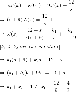
3\) Solve the differential equation

Solution
As we know that, Laplace transformation of


4\) Solve the differential equation,

Solution
As we know that,


5\) For circuit below, calculate the initial charging current of capacitor using Laplace Transform technique.

Solution
The above figure can be redrawn in Laplace form,


Now, initial charging current,

6\) Solve the [electric circuit](https://www.electrical4u.com/electric-circuit-or-electrical-network/) by using Laplace transformation for final steady-state current

Solution
The above circuit can be analyzed by using [Kirchhoff Voltage Law](https://www.electrical4u.com/kirchhoff-current-law-and-kirchhoff-voltage-law/) and then we get

Final value of steady-state current is

7\) A system is represented by the relation

Where, R(s) is the Laplace form of unit step function. Find the value of x(t) at t → ∞.
As R(s) is the Laplace form of unit step function, it can be written as
Solution

8\) Find f(t), f‘(t) and f“(t) for a time domain function f(t). The Laplace Transformation form of the function is given as

By applying initial value theorem, we get,


Applying Initial Value Theorem, we get,

9\) The Laplace Transform of f(t) is given by,

Find the final value of the equation using final value theorem as well as the conventional method of finding the final value.
Solution


Hence it is proved that from both of the methods the final value of the function becomes same.
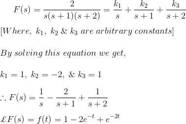
10\) Find the Inverse Laplace Transformation of function,

Solution
F(s) can be rewritten as,


11\) Find the Inverse Laplace transformation of

Solution
F(s) can be rewritten as,

12\) Find the Inverse Laplace transformation of

Solution
F(s) can be rewritten as,
13\) Express the differential equation in Laplace transformation form

Solution

14\) Express the differential equation in Laplace transformation form

Solution


## Where are Laplace Transforms used in Real Life?
Originating from Lerch’s Cancellation Law, the **Laplace Transform** converts time-domain functions into simpler algebraic equations in the frequency domain, which are easily solvable. These solutions are then converted back to the time domain using the Inverse Laplace Transform.
This transform is most commonly used for control systems, as briefly mentioned above. The transforms are used to study and analyze systems such as ventilation, heating and air conditions, etc. These systems are used in every single modern day construction and building.
Laplace transforms are also important for process controls. It aids in variable analysis which when altered produce the required results. An example of this can be found in experiments to do with heat.
Apart from these two examples, Laplace transforms are used in a lot of engineering applications and is a very useful method. It is useful in both electronic and mechanical engineering.
The control action for a dynamic control system whether electrical, mechanical, thermal, hydraulic, etc. can be represented by a differential equation. The system differential equation is derived according to physical laws governing is a system. In order to facilitate the solution of a differential equation describing a control system, the equation is transformed into an algebraic form. This transformation is done with the help of the **Laplace transformation** technique, that is the time domain differential equation is converted into a frequency domain algebraic equation.
An interesting analogy that may help in understanding Laplace is this. Imagine you come across an English poem which you do not understand. However, you have a Spanish friend who is excellent at making sense of these poems. So you translate this poem to Spanish and send it to him, he then in turn explains this poem in Spanish and sends it back to you. You understand the Spanish explanation and are then able to transfer the meaning of the poem back to English and thus understand the English poem.

About Electrical4U
Electrical4U is dedicated to the teaching and sharing of all things related to electrical and electronics engineering.
[...](https://www.electrical4u.com/author/electrical4u/ "Read more")
### Leave a Comment [Cancel reply](https://www.electrical4u.com/laplace-transformation/#respond)
Recent Posts
[Electric Current: What is it? (Formula, Units, AC vs DC)](https://www.electrical4u.com/electric-current-and-theory-of-electricity/)
[Voltage: What is it? (Definition, Formula And How To Measure Potential Difference)](https://www.electrical4u.com/voltage-or-electric-potential-difference/)
[Programmable Logic Controllers (PLCs): Basics, Types & Applications](https://www.electrical4u.com/programmable-logic-controllers/)
[Diode: Definition, Symbol, and Types of Diodes](https://www.electrical4u.com/diode-working-principle-and-types-of-diode/)
[Thermistor: Definition, Uses & How They Work](https://www.electrical4u.com/thermistor/)
[Half Wave Rectifier Circuit Diagram & Working Principle](https://www.electrical4u.com/half-wave-rectifiers/)
[Lenz’s Law of Electromagnetic Induction: Definition & Formula](https://www.electrical4u.com/lenz-law-of-electromagnetic-induction/)
[](https://www.electrical4u.com/best-electrical-engineering-books/)
[](https://www.electrical4u.com/electrical-engineering-app/)
Please feel free to [contact us](https://www.electrical4u.com/about/) if you’d like to request a specific topic. [Click here](https://www.electrical4u.com/privacy-policy/) to see our privacy policy.
We are a participant in the Amazon Services LLC Associates Program, an affiliate advertising program designed to provide a means for us to earn fees by linking to Amazon.com and affiliated sites. [Full disclaimer here](https://www.electrical4u.com/disclaimer/).
© 2025 [Electrical4U](https://www.electrical4u.com/) |
| Readable Markdown | Contents
💡
Key learnings:
- **Laplace Transform Definition**: The Laplace transform is a mathematical technique that converts a time-domain function into a frequency-domain function, simplifying the solving of differential equations.
- **Solving Process**: By transforming equations into the frequency domain, the Laplace transform simplifies complex differential calculations into more manageable algebraic forms.
- **Inverse Transformation**: The inverse Laplace transform allows the conversion of data from the frequency domain back to the original time-domain form, ensuring practical application of results.
- **Crucial Properties**: Understanding properties like linearity and time shifting is essential for effectively using Laplace transforms in system analysis and control.
- **Real-World Applications**: The Laplace transform is invaluable in engineering, particularly in designing and controlling systems where dynamic behavior modeling is required.
**Laplace transformation** is a technique for solving differential equations. Here differential equation of time domain form is first transformed to algebraic equation of frequency domain form. After solving the algebraic equation in frequency domain, the result then is finally transformed to time domain form to achieve the ultimate solution of the differential equation. In other words it can be said that the Laplace transformation is nothing but a shortcut method of solving differential equation.
In this article, we will be discussing Laplace transforms and how they are used to solve differential equations. They also provide a method to form a transfer function for an input-output system, but this shall not be discussed here. They provide the basic building blocks for control engineering, using block diagrams, etc.
Many kinds of transformations already exist but Laplace transforms and [Fourier transforms](https://www.electrical4u.com/fourier-series-and-fourier-transform/) are the most well known. The Laplace transforms is usually used to simplify a differential equation into a simple and solvable algebra problem. Even when the algebra becomes a little complex, it is still easier to solve than solving a differential equation.
There is always a table that is available to the engineer that contains information on the Laplace transforms. An example of **Laplace transform table** has been made below. We will come to know about the Laplace transform of various common functions from the following table .


## Laplace Transform Definition
When learning the Laplace transform, it’s important to understand not just the tables – but the formula too.
To understand the Laplace transform formula: First Let f(t) be the function of t, time for all t ≥ 0
Then the Laplace transform of f(t), F(s) can be defined as

Provided that the integral exists. Where the Laplace Operator, s = σ + jω; will be real or complex j = √(-1)
## Disadvantages of the Laplace Transformation Method
While powerful, the Laplace transform has limitations, such as being applicable only to differential equations with known constants. Without these constants, the method cannot be used, and alternative solutions must be sought.
## History of Laplace Transforms
The Laplace transform, named after the French mathematician and astronomer Pierre Simon Laplace, converts functions into different mathematical domains to solve otherwise intractable problems.
He used a similar transform on his additions to the probability theory. It became popular after World War Two. This transform was made popular by Oliver Heaviside, an English Electrical Engineer. Other famous scientists such as Niels Abel, Mathias Lerch, and Thomas Bromwich used it in the 19th century.
The complete history of the Laplace Transforms can be tracked a little more to the past, more specifically 1744. This is when another great mathematician called Leonhard Euler was researching on other types of integrals. Euler however did not pursue it very far and left it. An admirer of Euler called Joseph Lagrange; made some modifications to Euler’s work and did further work. LaGrange’s work got Laplace’s attention 38 years later, in 1782 where he continued to pick up where Euler left off. But it was not 3 years later; in 1785 where Laplace had a stroke of genius and changed the way we solve differential equations forever. He continued to work on it and continued to unlock the true power of the Laplace transform until 1809, where he started to use infinity as a integral condition.
## Method of Laplace Transform
In control system engineering, the Laplace transform is crucial for analyzing time functions. The inverse Laplace transform is equally important for deriving time-domain functions from their frequency-domain forms, with several properties beneficial for linear systems analysis.
Linearity, Differentiation, integration, multiplication, frequency shifting, time scaling, time shifting, convolution, conjugation, periodic function. There are two very important theorems associated with control systems. These are :
1. [Initial value theorem](https://www.electrical4u.com/initial-value-theorem-of-laplace-transform/) (IVT)
2. [Final value theorem](https://www.electrical4u.com/final-value-theorem-of-laplace-transform/) (FVT)
The Laplace transform is performed on a number of functions, which are – impulse, unit impulse, step, unit step, shifted unit step, ramp, exponential decay, sine, cosine, hyperbolic sine, hyperbolic cosine, natural logarithm, Bessel function. But the greatest advantage of applying the Laplace transform is solving higher order differential equations easily by converting into algebraic equations.
There are certain steps which need to be followed in order to do a Laplace transform of a time function. In order to transform a given function of time f(t) into its corresponding Laplace transform, we have to follow the following steps:
- First multiply f(t) by e\-st, s being a complex number (s = σ + j ω).
- Integrate this product w.r.t time with limits as zero and infinity. This integration results in Laplace transformation of f(t), which is denoted by F(s).

The time function f(t) is obtained back from the Laplace transform by a process called inverse Laplace transformation and denoted by £\-1

## Laplace Transform Properties
The main properties of Laplace Transform can be summarized as follows:
Linearity: Let C1, C2 be constants. f(t), g(t) be the functions of time, t, then

First shifting Theorem:

Change of scale property:

Differentiation:

Integration:

Time Shifting:
If L{f(t) } = F(s), then the Laplace Transform of f(t) after the delay of time, T is equal to the product of Laplace Transform of f(t) and e\-st that is

Where, u(t-T) denotes unit step function.
Product:
If L{f(t) }=F(s), then the product of two functions, f1 (t) and f2 (t) is

Final Value Theorem:

This theorem is applicable in the analysis and design of feedback control system, as Laplace Transform gives solution at initial conditions
Initial Value Theorem:

Let us examine the Laplace transformation methods of a simple function f(t) = eαt for better understanding the matter.

Comparing the above solution, we can write,

Similarly, by putting α = 0, we get,

Similarly, by putting α = jω, we get,


And thus,

Let us examine another [example of Laplace transformation](https://www.electrical4u.com/laplace-transformation/) methods for the function


Again the Laplace transformation form of et is,

This Laplace form can be rewritten as

Now from the definition of power series we get,


## Laplace Transform Examples
Solve the equation using **Laplace Transforms**,

Using the table above, the equation can be converted into Laplace form:

Using the data that has been given in the question the Laplace form can be simplified.

Dividing by (s2 + 3s + 2) gives

This can be solved using partial fractions, which is easier than solving it in its previous form. Firstly, the denominator needs to be factorized.

Cross-multiplying gives:

Next the coefficients A and B need to be found

Substituting in the equation:

Then using the table that was provided above, that equation can be converted back into normal form.
Examples to try yourself
Calculate and write out the inverse Laplace transformation of the following, it is recommended to find a table with the Laplace conversions online:

Solutions:

Let’s dig in a bit more into some worked laplace transform examples:
1\) Where, F(s) is the Laplace form of a time domain function f(t). Find the expiration of f(t).

Solution

Now, Inverse Laplace Transformation of F(s), is

2\) Find Inverse Laplace Transformation function of

Solution

Now,


Hence,

3\) Solve the differential equation

Solution
As we know that, Laplace transformation of


4\) Solve the differential equation,

Solution
As we know that,


5\) For circuit below, calculate the initial charging current of capacitor using Laplace Transform technique.

Solution
The above figure can be redrawn in Laplace form,


Now, initial charging current,

6\) Solve the [electric circuit](https://www.electrical4u.com/electric-circuit-or-electrical-network/) by using Laplace transformation for final steady-state current

Solution
The above circuit can be analyzed by using [Kirchhoff Voltage Law](https://www.electrical4u.com/kirchhoff-current-law-and-kirchhoff-voltage-law/) and then we get

Final value of steady-state current is

7\) A system is represented by the relation

Where, R(s) is the Laplace form of unit step function. Find the value of x(t) at t → ∞.
As R(s) is the Laplace form of unit step function, it can be written as
Solution

8\) Find f(t), f‘(t) and f“(t) for a time domain function f(t). The Laplace Transformation form of the function is given as

By applying initial value theorem, we get,


Applying Initial Value Theorem, we get,

9\) The Laplace Transform of f(t) is given by,

Find the final value of the equation using final value theorem as well as the conventional method of finding the final value.
Solution


Hence it is proved that from both of the methods the final value of the function becomes same.
10\) Find the Inverse Laplace Transformation of function,

Solution
F(s) can be rewritten as,


11\) Find the Inverse Laplace transformation of

Solution
F(s) can be rewritten as,

12\) Find the Inverse Laplace transformation of

Solution
F(s) can be rewritten as,

13\) Express the differential equation in Laplace transformation form

Solution

14\) Express the differential equation in Laplace transformation form

Solution


## Where are Laplace Transforms used in Real Life?
Originating from Lerch’s Cancellation Law, the **Laplace Transform** converts time-domain functions into simpler algebraic equations in the frequency domain, which are easily solvable. These solutions are then converted back to the time domain using the Inverse Laplace Transform.
This transform is most commonly used for control systems, as briefly mentioned above. The transforms are used to study and analyze systems such as ventilation, heating and air conditions, etc. These systems are used in every single modern day construction and building.
Laplace transforms are also important for process controls. It aids in variable analysis which when altered produce the required results. An example of this can be found in experiments to do with heat.
Apart from these two examples, Laplace transforms are used in a lot of engineering applications and is a very useful method. It is useful in both electronic and mechanical engineering.
The control action for a dynamic control system whether electrical, mechanical, thermal, hydraulic, etc. can be represented by a differential equation. The system differential equation is derived according to physical laws governing is a system. In order to facilitate the solution of a differential equation describing a control system, the equation is transformed into an algebraic form. This transformation is done with the help of the **Laplace transformation** technique, that is the time domain differential equation is converted into a frequency domain algebraic equation.
An interesting analogy that may help in understanding Laplace is this. Imagine you come across an English poem which you do not understand. However, you have a Spanish friend who is excellent at making sense of these poems. So you translate this poem to Spanish and send it to him, he then in turn explains this poem in Spanish and sends it back to you. You understand the Spanish explanation and are then able to transfer the meaning of the poem back to English and thus understand the English poem. |
| Shard | 192 (laksa) |
| Root Hash | 15046430122061128792 |
| Unparsed URL | com,electrical4u!www,/laplace-transformation/ s443 |