ℹ️ Skipped - page is already crawled
| Filter | Status | Condition | Details |
|---|---|---|---|
| HTTP status | PASS | download_http_code = 200 | HTTP 200 |
| Age cutoff | PASS | download_stamp > now() - 6 MONTH | 0 months ago |
| History drop | PASS | isNull(history_drop_reason) | No drop reason |
| Spam/ban | PASS | fh_dont_index != 1 AND ml_spam_score = 0 | ml_spam_score=0 |
| Canonical | PASS | meta_canonical IS NULL OR = '' OR = src_unparsed | Not set |
| Property | Value | ||||||||||||||||||
|---|---|---|---|---|---|---|---|---|---|---|---|---|---|---|---|---|---|---|---|
| URL | https://www.datacamp.com/tutorial/tensorflow-tutorial | ||||||||||||||||||
| Last Crawled | 2026-04-23 13:18:29 (9 hours ago) | ||||||||||||||||||
| First Indexed | 2022-04-15 02:55:30 (4 years ago) | ||||||||||||||||||
| HTTP Status Code | 200 | ||||||||||||||||||
| Content | |||||||||||||||||||
| Meta Title | TensorFlow Tutorial For Beginners | DataCamp | ||||||||||||||||||
| Meta Description | In this TensorFlow beginner tutorial, you'll learn how to build a neural network step-by-step and how to train, evaluate and optimize it. | ||||||||||||||||||
| Meta Canonical | null | ||||||||||||||||||
| Boilerpipe Text | Deep learning is a subfield of machine learning that is a set of algorithms that is inspired by the structure and function of the brain.
TensorFlow is the second machine learning framework that Google created and used to design, build, and train deep learning models. You can use the TensorFlow library do to numerical computations, which in itself doesn’t seem all too special, but these computations are done with data flow graphs. In these graphs, nodes represent mathematical operations, while the edges represent the data, which usually are multidimensional data arrays or tensors, that are communicated between these edges.
You see? The name “TensorFlow” is derived from the operations which neural networks perform on multidimensional data arrays or tensors! It’s literally a flow of tensors. For now, this is all you need to know about tensors, but you’ll go deeper into this in the next sections!
Today’s TensorFlow tutorial for beginners will introduce you to performing deep learning in an interactive way:
You’ll first learn more about
tensors
;
Then, the tutorial you’ll briefly go over some of the ways that you can
install TensorFlow
on your system so that you’re able to get started and load data in your workspace;
After this, you’ll go over some of the
TensorFlow basics
: you’ll see how you can easily get started with simple computations.
After this, you get started on the real work: you’ll load in data on
Belgian traffic signs
and
exploring
it with simple statistics and plotting.
In your exploration, you’ll see that there is a need to
manipulate your data
in such a way that you can feed it to your model. That’s why you’ll take the time to rescale your images and convert them to grayscale.
Next, you can finally get started on
your neural network model
! You’ll build up your model layer per layer;
Once the architecture is set up, you can use it to
train your model interactively
and to eventually also
evaluate
it by feeding some test data to it.
Lastly, you’ll get some pointers for
further
improvements that you can do to the model you just constructed and how you can continue your learning with TensorFlow.
Download the notebook of this tutorial
here
.
Also, you could be interested in a course on
Deep Learning in Python
, DataCamp's
Keras tutorial
or the
keras with R tutorial
.
Introducing Tensors
To understand tensors well, it’s good to have some working knowledge of linear algebra and vector calculus. You already read in the introduction that tensors are implemented in TensorFlow as multidimensional data arrays, but some more introduction is maybe needed in order to completely grasp tensors and their use in machine learning.
Plane Vectors
Before you go into plane vectors, it’s a good idea to shortly revise the concept of “vectors”; Vectors are special types of matrices, which are rectangular arrays of numbers. Because vectors are ordered collections of numbers, they are often seen as column matrices: they have just one column and a certain number of rows. In other terms, you could also consider vectors as scalar magnitudes that have been given a direction.
Remember
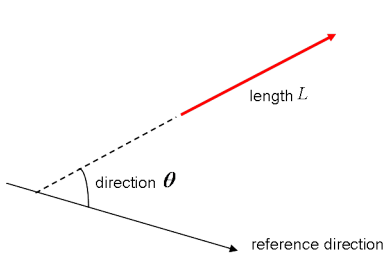
: an example of a scalar is “5 meters” or “60 m/sec”, while a vector is, for example, “5 meters north” or “60 m/sec East”. The difference between these two is obviously that the vector has a direction. Nevertheless, these examples that you have seen up until now might seem far off from the vectors that you might encounter when you’re working with machine learning problems. This is normal; The length of a mathematical vector is a pure number: it is absolute. The direction, on the other hand, is relative: it is measured relative to some reference direction and has units of radians or degrees. You usually assume that the direction is positive and in counterclockwise rotation from the reference direction.
Visually, of course, you represent vectors as arrows, as you can see in the picture above. This means that you can consider vectors also as arrows that have direction and length. The direction is indicated by the arrow’s head, while the length is indicated by the length of the arrow.
So what about plane vectors then?
Plane vectors are the most straightforward setup of tensors. They are much like regular vectors as you have seen above, with the sole difference that they find themselves in a vector space. To understand this better, let’s start with an example: you have a vector that is
2 X 1
. This means that the vector belongs to the set of real numbers that come paired two at a time. Or, stated differently, they are part of two-space. In such cases, you can represent vectors on the coordinate
(x,y)
plane with arrows or rays.
Working from this coordinate plane in a standard position where vectors have their endpoint at the origin
(0,0)
, you can derive the
x
coordinate by looking at the first row of the vector, while you’ll find the
y
coordinate in the second row. Of course, this standard position doesn’t always need to be maintained: vectors can move parallel to themselves in the plane without experiencing changes.
Note
that similarly, for vectors that are of size
3 X 1
, you talk about the three-space. You can represent the vector as a three-dimensional figure with arrows pointing to positions in the vectors pace: they are drawn on the standard
x
,
y
and
z
axes.
It’s nice to have these vectors and to represent them on the coordinate plane, but in essence, you have these vectors so that you can perform operations on them and one thing that can help you in doing this is by expressing your vectors as bases or unit vectors.
Unit vectors are vectors with a magnitude of one. You’ll often recognize the unit vector by a lowercase letter with a circumflex, or “hat”. Unit vectors will come in convenient if you want to express a 2-D or 3-D vector as a sum of two or three orthogonal components, such as the x− and y−axes, or the z−axis.
And when you are talking about expressing one vector, for example, as sums of components, you’ll see that you’re talking about component vectors, which are two or more vectors whose sum is that given vector.
Tip
: watch
this video
, which explains what tensors are with the help of simple household objects!
Tensors
Next to plane vectors, also covectors and linear operators are two other cases that all three together have one thing in common: they are specific cases of tensors. You still remember how a vector was characterized in the previous section as scalar magnitudes that have been given a direction. A tensor, then, is the mathematical representation of a physical entity that may be characterized by magnitude and
multiple
directions.
And, just like you represent a scalar with a single number and a vector with a sequence of three numbers in a 3-dimensional space, for example, a tensor can be represented by an array of 3R numbers in a 3-dimensional space.
The “R” in this notation represents the rank of the tensor: this means that in a 3-dimensional space, a second-rank tensor can be represented by 3 to the power of 2 or 9 numbers. In an N-dimensional space, scalars will still require only one number, while vectors will require N numbers, and tensors will require N^R numbers. This explains why you often hear that scalars are tensors of rank 0: since they have no direction, you can represent them with one number.
With this in mind, it’s relatively easy to recognize scalars, vectors, and tensors and to set them apart: scalars can be represented by a single number, vectors by an ordered set of numbers, and tensors by an array of numbers.
What makes tensors so unique is the combination of components and basis vectors: basis vectors transform one way between reference frames and the components transform in just such a way as to keep the combination between components and basis vectors the same.
Installing TensorFlow
Now that you know more about TensorFlow, it’s time to get started and install the library. Here, it’s good to know that TensorFlow provides APIs for Python, C++, Haskell, Java, Go, Rust, and there’s also a third-party package for R called
tensorflow
.
Tip
: if you want to know more about deep learning packages in R, consider checking out DataCamp’s
keras: Deep Learning in R Tutorial
.
In this tutorial, you will download a version of TensorFlow that will enable you to write the code for your deep learning project in Python. On the
TensorFlow installation webpage
, you’ll see some of the most common ways and latest instructions to install TensorFlow using
virtualenv
,
pip
, Docker and lastly, there are also some of the other ways of installing TensorFlow on your personal computer.
Note
You can also install TensorFlow with Conda if you’re working on Windows. However, since the installation of TensorFlow is community supported, it’s best to check the
official installation instructions
.
Now that you have gone through the installation process, it’s time to double check that you have installed TensorFlow correctly by importing it into your workspace under the alias
tf
:
import
tensorflow
as
tf
Was this AI assistant helpful?
Note
that the alias that you used in the line of code above is sort of a convention - It’s used to ensure that you remain consistent with other developers that are using TensorFlow in data science projects on the one hand, and with open-source TensorFlow projects on the other hand.
Getting Started with TensorFlow: Basics
You’ll generally write TensorFlow programs, which you run as a chunk; This is at first sight kind of contradictory when you’re working with Python. However, if you would like, you can also use TensorFlow’s Interactive Session, which you can use to work more interactively with the library. This is especially handy when you’re used to working with IPython.
For this tutorial, you’ll focus on the second option: this will help you to get kickstarted with deep learning in TensorFlow. But before you go any further into this, let’s first try out some minor stuff before you start with the heavy lifting.
First, import the
tensorflow
library under the alias
tf
, as you have seen in the previous section. Then initialize two variables that are actually constants. Pass an array of four numbers to the
constant
(
)
function.
Note
that you could potentially also pass in an integer, but that more often than not, you’ll find yourself working with arrays. As you saw in the introduction, tensors are all about arrays! So make sure that you pass in an array :) Next, you can use
multiply
(
)
to multiply your two variables. Store the result in the
result
variable. Lastly, print out the
result
with the help of the
print
(
)
function.
script.py
7
IPython Shell
Note
that you have defined constants in the DataCamp Light code chunk above. However, there are two other types of values that you can potentially use, namely
placeholders
, which are values that are unassigned and that will be initialized by the session when you run it. Like the name already gave away, it’s just a placeholder for a tensor that will always be fed when the session is run; There are also
Variables
, which are values that can change. The constants, as you might have already gathered, are values that don’t change.
The result of the lines of code is an abstract tensor in the computation graph. However, contrary to what you might expect, the
result
doesn’t actually get calculated. It just defined the model, but no process ran to calculate the result. You can see this in the print-out: there’s not really a result that you want to see (namely, 30). This means that TensorFlow has a lazy evaluation!
However, if you do want to see the result, you have to run this code in an interactive session. You can do this in a few ways, as is demonstrated in the DataCamp Light code chunks below:
script.py
10
IPython Shell
Note
that you can also use the following lines of code to start up an interactive Session, run the
result
and close the Session automatically again after printing the
output
:
script.py
8
IPython Shell
In the code chunks above you have just defined a default Session, but it’s also good to know that you can pass in options as well. You can, for example, specify the
config
argument and then use the
ConfigProto
protocol buffer to add configuration options for your session.
For example, if you add
config
=
tf
.
ConfigProto
(
log_device_placement
=
True
)
Was this AI assistant helpful?
to your Session, you make sure that you log the GPU or CPU device that is assigned to an operation. You will then get information which devices are used in the session for each operation. You could use the following configuration session also, for example, when you use soft constraints for the device placement:
config
=
tf
.
ConfigProto
(
allow_soft_placement
=
True
)
Was this AI assistant helpful?
Now that you’ve got TensorFlow installed and imported into your workspace and you’ve gone through the basics of working with this package, it’s time to leave this aside for a moment and turn your attention to your data. Just like always, you’ll first take your time to explore and understand your data better before you start modeling your neural network.
Belgian Traffic Signs: Background
Even though traffic is a topic that is generally known amongst you all, it doesn’t hurt going briefly over the observations that are included in this dataset to see if you understand everything before you start. In essence, in this section, you’ll get up to speed with the domain knowledge that you need to have to go further with this tutorial.
Of course, because I’m Belgian, I’ll make sure you’ll also get some anecdotes :)
Belgian traffic signs are usually in Dutch and French. This is good to know, but for the dataset that you’ll be working with, it’s not too important!
There are six categories of traffic signs in Belgium: warning signs, priority signs, prohibitory signs, mandatory signs, signs related to parking and standing still on the road and, lastly, designatory signs.
On January 1st, 2017, more than 30,000 traffic signs were removed from Belgian roads. These were all prohibitory signs relating to speed.
Talking about removal, the overwhelming presence of traffic signs has been an ongoing discussion in Belgium (and by extension, the entire European Union).
Loading and Exploring the Data
Now that you have gathered some more background information, it’s time to download the dataset
here
. You should get the two zip files listed next to "BelgiumTS for Classification (cropped images), which are called "BelgiumTSC_Training" and "BelgiumTSC_Testing".
Tip
: if you have downloaded the files or will do so after completing this tutorial, take a look at the folder structure of the data that you’ve downloaded! You’ll see that the testing, as well as the training data folders, contain 61 subfolders, which are the 62 types of traffic signs that you’ll use for classification in this tutorial. Additionally, you’ll find that the files have the file extension
.
ppm
or Portable Pixmap Format. You have downloaded images of the traffic signs!
Let’s get started with importing the data into your workspace. Let’s start with the lines of code that appear below the User-Defined Function (UDF)
load_data
(
)
:
First, set your
ROOT_PATH
. This path is the one where you have made the directory with your training and test data.
Next, you can add the specific paths to your
ROOT_PATH
with the help of the
join
(
)
function. You store these two specific paths in
train_data_directory
and
test_data_directory
.
You see that after, you can call the
load_data
(
)
function and pass in the
train_data_directory
to it.
Now, the
load_data
(
)
function itself starts off by gathering all the subdirectories that are present in the
train_data_directory
; It does so with the help of list comprehension, which is quite a natural way of constructing lists - it basically says that, if you find something in the
train_data_directory
, you’ll double check whether this is a directory, and if it is one, you’ll add it to your list.
Remember
that each subdirectory represents a label.
Next, you have to loop through the subdirectories. You first initialize two lists,
labels
and
images
. Next, you gather the paths of the subdirectories and the file names of the images that are stored in these subdirectories. After, you can collect the data in the two lists with the help of the
append
(
)
function.
def
load_data
(
data_directory
)
:
directories
=
[
d
for
d
in
os
.
listdir
(
data_directory
)
if
os
.
path
.
isdir
(
os
.
path
.
join
(
data_directory
,
d
)
)
]
labels
=
[
]
images
=
[
]
for
d
in
directories
:
label_directory
=
os
.
path
.
join
(
data_directory
,
d
)
file_names
=
[
os
.
path
.
join
(
label_directory
,
f
)
for
f
in
os
.
listdir
(
label_directory
)
if
f
.
endswith
(
".ppm"
)
]
for
f
in
file_names
:
images
.
append
(
skimage
.
data
.
imread
(
f
)
)
labels
.
append
(
int
(
d
)
)
return
images
,
labels
ROOT_PATH
=
"/your/root/path"
train_data_directory
=
os
.
path
.
join
(
ROOT_PATH
,
"TrafficSigns/Training"
)
test_data_directory
=
os
.
path
.
join
(
ROOT_PATH
,
"TrafficSigns/Testing"
)
images
,
labels
=
load_data
(
train_data_directory
)
Was this AI assistant helpful?
Note
that in the above code chunk, the training and test data are located in folders named "Training" and "Testing", which are both subdirectories of another directory "TrafficSigns". On a local machine, this could look something like "/Users/Name/Downloads/TrafficSigns", with then two subfolders called "Training" and "Testing".
Tip
: review how to write functions in Python with DataCamp's
Python Functions Tutorial
.
Traffic Sign Statistics
With your data loaded in, it’s time for some data inspection! You can start with a pretty simple analysis with the help of the
ndim
and
size
attributes of the
images
array:
Note that the
images
and
labels
variables are lists, so you might need to use
np
.
array
(
)
to convert the variables to an array in your own workspace. This has been done for you here!
script.py
5
IPython Shell
Note
that the
images
[
0
]
that you printed out is, in fact, one single image that is represented by arrays in arrays! This might seem counterintuitive at first, but it’s something that you’ll get used to as you go further into working with images in machine learning or deep learning applications.
Next, you can also take a small look at the
labels
, but you shouldn’t see too many surprises at this point:
script.py
5
IPython Shell
These numbers already give you some insights into how successful your import was and the exact size of your data. At first sight, everything has been executed the way you expected it to, and you see that the size of the array is considerable if you take into account that you’re dealing with arrays within arrays.
Tip
try adding the following attributes to your arrays to get more information about the memory layout, the length of one array element in bytes and the total consumed bytes by the array’s elements with the
flags
,
itemsize
, and
nbytes
attributes. You can test this out in the IPython console in the DataCamp Light chunk above!
Next, you can also take a look at the distribution of the traffic signs:
script.py
5
IPython Shell
Awesome job! Now let’s take a closer look at the histogram that you made!
You clearly see that not all types of traffic signs are equally represented in the dataset. This is something that you’ll deal with later when you’re manipulating the data before you start modeling your neural network.
At first sight, you see that there are labels that are more heavily present in the dataset than others: the labels 22, 32, 38, and 61 definitely jump out. At this point, it’s nice to keep this in mind, but you’ll definitely go further into this in the next section!
Visualizing the Traffic Signs
The previous, small analyses or checks have already given you some idea of the data that you’re working with, but when your data mostly consists of images, the step that you should take to explore your data is by visualizing it.
Let’s check out some random traffic signs:
First, make sure that you import the
pyplot
module of the
matplotlib
package under the common alias
plt
.
Then, you’re going to make a list with 4 random numbers. These will be used to select traffic signs from the
images
array that you have just inspected in the previous section. In this case, you go for
300
,
2250
,
3650
and
4000
.
Next, you’ll say that for every element in the length of that list, so from 0 to 4, you’re going to create subplots without axes (so that they don’t go running with all the attention and your focus is solely on the images!). In these subplots, you’re going to show a specific image from the
images
array that is in accordance with the number at the index
i
. In the first loop, you’ll pass
300
to
images
[
]
, in the second round
2250
, and so on. Lastly, you’ll adjust the subplots so that there’s enough width in between them.
The last thing that remains is to show your plot with the help of the
show
(
)
function!
There you go:
# Import the `pyplot` module of `matplotlib`
import
matplotlib
.
pyplot
as
plt
# Determine the (random) indexes of the images that you want to see
traffic_signs
=
[
300
,
2250
,
3650
,
4000
]
# Fill out the subplots with the random images that you defined
for
i
in
range
(
len
(
traffic_signs
)
)
:
plt
.
subplot
(
1
,
4
,
i
+
1
)
plt
.
axis
(
'off'
)
plt
.
imshow
(
images
[
traffic_signs
[
i
]
]
)
plt
.
subplots_adjust
(
wspace
=
0.5
)
plt
.
show
(
)
Was this AI assistant helpful?
As you guessed by the 62 labels that are included in this dataset, the signs are different from each other.
But what else do you notice? Take another close look at the images below:
These four images are not of the same size!
You can obviously toy around with the numbers that are contained in the
traffic_signs
list and follow up more thoroughly on this observation, but be as it may, this is an important observation which you will need to take into account when you start working more towards manipulating your data so that you can feed it to the neural network.
Let’s confirm the hypothesis of the differing sizes by printing the shape, the minimum and maximum values of the specific images that you have included into the subplots.
The code below heavily resembles the one that you used to create the above plot, but differs in the fact that here, you’ll alternate sizes and images instead of plotting just the images next to each other:
# Import `matplotlib`
import
matplotlib
.
pyplot
as
plt
# Determine the (random) indexes of the images
traffic_signs
=
[
300
,
2250
,
3650
,
4000
]
# Fill out the subplots with the random images and add shape, min and max values
for
i
in
range
(
len
(
traffic_signs
)
)
:
plt
.
subplot
(
1
,
4
,
i
+
1
)
plt
.
axis
(
'off'
)
plt
.
imshow
(
images
[
traffic_signs
[
i
]
]
)
plt
.
subplots_adjust
(
wspace
=
0.5
)
plt
.
show
(
)
print
(
"shape: {0}, min: {1}, max: {2}"
.
format
(
images
[
traffic_signs
[
i
]
]
.
shape
,
images
[
traffic_signs
[
i
]
]
.
min
(
)
,
images
[
traffic_signs
[
i
]
]
.
max
(
)
)
)
Was this AI assistant helpful?
Note
how you use the
format
(
)
method on the string
"shape: {0}, min: {1}, max: {2}"
to fill out the arguments
{
0
}
,
{
1
}
, and
{
2
}
that you defined.
Now that you have seen loose images, you might also want to revisit the histogram that you printed out in the first steps of your data exploration; You can easily do this by plotting an overview of all the 62 classes and one image that belongs to each class:
# Import the `pyplot` module as `plt`
import
matplotlib
.
pyplot
as
plt
# Get the unique labels
unique_labels
=
set
(
labels
)
# Initialize the figure
plt
.
figure
(
figsize
=
(
15
,
15
)
)
# Set a counter
i
=
1
# For each unique label,
for
label
in
unique_labels
:
# You pick the first image for each label
image
=
images
[
labels
.
index
(
label
)
]
# Define 64 subplots
plt
.
subplot
(
8
,
8
,
i
)
# Don't include axes
plt
.
axis
(
'off'
)
# Add a title to each subplot
plt
.
title
(
"Label {0} ({1})"
.
format
(
label
,
labels
.
count
(
label
)
)
)
# Add 1 to the counter
i
+=
1
# And you plot this first image
plt
.
imshow
(
image
)
# Show the plot
plt
.
show
(
)
Was this AI assistant helpful?
Note
that even though you define 64 subplots, not all of them will show images (as there are only 62 labels!). Note also that again, you don’t include any axes to make sure that the readers’ attention doesn’t dwell far from the main topic: the traffic signs!
As you mostly guessed in the histogram above, there are considerably more traffic signs with labels 22, 32, 38, and 61. This hypothesis is now confirmed in this plot: you see that there are 375 instances with label 22, 316 instances with label 32, 285 instances with label 38 and, lastly, 282 instances with label 61.
One of the most interesting questions that you could ask yourself now is whether there’s a connection between all of these instances - maybe all of them are designatory signs?
Let’s take a closer look: you see that label 22 and 32 are prohibitory signs, but that labels 38 and 61 are designatory and a prioritory signs, respectively. This means that there’s not an immediate connection between these four, except for the fact that half of the signs that have a substantial presence in the dataset is of the prohibitory kind.
Feature Extraction
Now that you have thoroughly explored your data, it’s time to get your hands dirty! Let’s recap briefly what you discovered to make sure that you don’t forget any steps in the manipulation:
The size of the images was unequal;
There are 62 labels or target values (as your labels start at 0 and end at 61);
The distribution of the traffic sign values is pretty unequal; There wasn’t really any connection between the signs that were heavily present in the dataset.
Now that you have a clear idea of what you need to improve, you can start with manipulating your data in such a way that it’s ready to be fed to the neural network or whichever model you want to feed it too. Let’s start first with extracting some features - you’ll rescale the images, and you’ll convert the images that are held in the
images
array to grayscale. You’ll do this color conversion mainly because the color matters less in classification questions like the one you’re trying to answer now. For detection, however, the color does play a big part! So in those cases, it’s not needed to do that conversion!
Rescaling Images
To tackle the differing image sizes, you’re going to rescale the images; You can easily do this with the help of the
skimage
or Scikit-Image library, which is a collection of algorithms for image processing.
In this case, the
transform
module will come in handy, as it offers you a
resize
(
)
function; You’ll see that you make use of list comprehension (again!) to resize each image to 28 by 28 pixels. Once again, you see that the way you actually form the list: for every image that you find in the
images
array, you’ll perform the transformation operation that you borrow from the
skimage
library. Finally, you store the result in the
images28
variable:
# Import the `transform` module from `skimage`
from
skimage
import
transform
# Rescale the images in the `images` array
images28
=
[
transform
.
resize
(
image
,
(
28
,
28
)
)
for
image
in
images
]
Was this AI assistant helpful?
This was fairly easy wasn’t it?
Note
that the images are now four-dimensional: if you convert
images28
to an array and if you concatenate the attribute
shape
to it, you’ll see that the printout tells you that
images28
’s dimensions are
(
4575
,
28
,
28
,
3
)
. The images are 784-dimensional (because your images are 28 by 28 pixels).
You can check the result of the rescaling operation by re-using the code that you used above to plot the 4 random images with the help of the
traffic_signs
variable. Just don’t forget to change all references to
images
to
images28
.
Check out the result here:
Note
that because you rescaled, your
min
and
max
values have also changed; They seem to be all in the same ranges now, which is really great because then you don’t necessarily need to normalize your data!
Image Conversion to Grayscale
As said in the introduction to this section of the tutorial, the color in the pictures matters less when you’re trying to answer a classification question. That’s why you’ll also go through the trouble of converting the images to grayscale.
Note
, however, that you can also test out on your own what would happen to the final results of your model if you don’t follow through with this specific step.
Just like with the rescaling, you can again count on the Scikit-Image library to help you out; In this case, it’s the
color
module with its
rgb2gray
(
)
function that you need to use to get where you need to be.
That’s going to be nice and easy!
However, don’t forget to convert the
images28
variable back to an array, as the
rgb2gray
(
)
function does expect an array as an argument.
# Import `rgb2gray` from `skimage.color`
from
skimage
.
color
import
rgb2gray
# Convert `images28` to an array
images28
=
np
.
array
(
images28
)
# Convert `images28` to grayscale
images28
=
rgb2gray
(
images28
)
Was this AI assistant helpful?
Double check the result of your grayscale conversion by plotting some of the images; Here, you can again re-use and slightly adapt some of the code to show the adjusted images:
import
matplotlib
.
pyplot
as
plt
traffic_signs
=
[
300
,
2250
,
3650
,
4000
]
for
i
in
range
(
len
(
traffic_signs
)
)
:
plt
.
subplot
(
1
,
4
,
i
+
1
)
plt
.
axis
(
'off'
)
plt
.
imshow
(
images28
[
traffic_signs
[
i
]
]
,
cmap
=
"gray"
)
plt
.
subplots_adjust
(
wspace
=
0.5
)
# Show the plot
plt
.
show
(
)
Was this AI assistant helpful?
Note
that you indeed have to specify the color map or
cmap
and set it to
"gray"
to plot the images in grayscale. That is because
imshow
(
)
by default uses, by default, a heatmap-like color map. Read more
here
.
Tip
: since you have been re-using this function quite a bit in this tutorial, you might look into how you can make it into a function :)
These two steps are very basic ones; Other operations that you could have tried out on your data include data augmentation (rotating, blurring, shifting, changing brightness,…). If you want, you could also set up an entire pipeline of data manipulation operations through which you send your images.
Deep Learning with TensorFlow
Now that you have explored and manipulated your data, it’s time to construct your neural network architecture with the help of the TensorFlow package!
Modeling the Neural Network
Just like you might have done with Keras, it’s time to build up your neural network, layer by layer.
If you haven’t done so already, import
tensorflow
into your workspace under the conventional alias
tf
. Then, you can initialize the Graph with the help of
Graph
(
)
. You use this function to define the computation.
Note
that with the Graph, you don’t compute anything, because it doesn’t hold any values. It just defines the operations that you want to be running later.
In this case, you set up a default context with the help of
as_default
(
)
, which returns a context manager that makes this specific Graph the default graph. You use this method if you want to create multiple graphs in the same process: with this function, you have a global default graph to which all operations will be added if you don’t explicitly create a new graph.
Next, you’re ready to add operations to your graph. As you might remember from working with Keras, you build up your model, and then in compiling it, you define a loss function, an optimizer, and a metric. This now all happens in one step when you work with TensorFlow:
First, you define placeholders for inputs and labels because you won’t put in the “real” data yet.
Remember
that placeholders are values that are unassigned and that will be initialized by the session when you run it. So when you finally run the session, these placeholders will get the values of your dataset that you pass in the
run
(
)
function!
Then, you build up the network. You first start by flattening the input with the help of the
flatten
(
)
function, which will give you an array of shape
[
None
,
784
]
instead of the
[
None
,
28
,
28
]
, which is the shape of your grayscale images.
After you have flattened the input, you construct a fully connected layer that generates logits of size
[
None
,
62
]
. Logits is the function operates on the unscaled output of previous layers, and that uses the relative scale to understand the units is linear.
With the multi-layer perceptron built out, you can define the loss function. The choice for a loss function depends on the task that you have at hand: in this case, you make use of
sparse_softmax_cross_entropy_with_logits
(
)
Was this AI assistant helpful?
This computes sparse softmax cross entropy between logits and labels. In other words, it measures the probability error in discrete classification tasks in which the classes are mutually exclusive. This means that each entry is in exactly one class. Here, a traffic sign can only have one single label.
Remember
that, while regression is used to predict continuous values, classification is used to predict discrete values or classes of data points. You wrap this function with
reduce_mean
(
)
, which computes the mean of elements across dimensions of a tensor.
You also want to define a training optimizer; Some of the most popular optimization algorithms used are the Stochastic Gradient Descent (SGD), ADAM and RMSprop. Depending on whichever algorithm you choose, you’ll need to tune certain parameters, such as learning rate or momentum. In this case, you pick the ADAM optimizer, for which you define the learning rate at
0.001
.
Lastly, you initialize the operations to execute before going over to the training.
# Import `tensorflow`
import
tensorflow
as
tf
# Initialize placeholders
x
=
tf
.
placeholder
(
dtype
=
tf
.
float32
,
shape
=
[
None
,
28
,
28
]
)
y
=
tf
.
placeholder
(
dtype
=
tf
.
int32
,
shape
=
[
None
]
)
# Flatten the input data
images_flat
=
tf
.
contrib
.
layers
.
flatten
(
x
)
# Fully connected layer
logits
=
tf
.
contrib
.
layers
.
fully_connected
(
images_flat
,
62
,
tf
.
nn
.
relu
)
# Define a loss function
loss
=
tf
.
reduce_mean
(
tf
.
nn
.
sparse_softmax_cross_entropy_with_logits
(
labels
=
y
,
logits
=
logits
)
)
# Define an optimizer
train_op
=
tf
.
train
.
AdamOptimizer
(
learning_rate
=
0.001
)
.
minimize
(
loss
)
# Convert logits to label indexes
correct_pred
=
tf
.
argmax
(
logits
,
1
)
# Define an accuracy metric
accuracy
=
tf
.
reduce_mean
(
tf
.
cast
(
correct_pred
,
tf
.
float32
)
)
Was this AI assistant helpful?
You have now successfully created your first neural network with TensorFlow!
If you want, you can also print out the values of (most of) the variables to get a quick recap or checkup of what you have just coded up:
print
(
"images_flat: "
,
images_flat
)
print
(
"logits: "
,
logits
)
print
(
"loss: "
,
loss
)
print
(
"predicted_labels: "
,
correct_pred
)
Was this AI assistant helpful?
Tip
: if you see an error like “
module
'pandas'
has no attribute
'computation'
”, consider upgrading the packages
dask
by running
pip install
-
-
upgrade dask
in your command line. See
this StackOverflow post
for more information.
Running the Neural Network
Now that you have built up your model layer by layer, it’s time to actually run it! To do this, you first need to initialize a session with the help of
Session
(
)
to which you can pass your
graph
that you defined in the previous section. Next, you can run the session with
run
(
)
, to which you pass the initialized operations in the form of the
init
variable that you also defined in the previous section.
Next, you can use this initialized session to start epochs or training loops. In this case, you pick
201
because you want to be able to register the last
loss_value
; In the loop, you run the session with the training optimizer and the loss (or accuracy) metric that you defined in the previous section. You also pass a
feed_dict
argument, with which you feed data to the model. After every 10 epochs, you’ll get a log that gives you more insights into the loss or cost of the model.
As you have seen in the section on the TensorFlow basics, there is no need to close the session manually; this is done for you. However, if you want to try out a different setup, you probably will need to do so with
sess
.
close
(
)
if you have defined your session as
sess
, like in the code chunk below:
tf
.
set_random_seed
(
1234
)
sess
=
tf
.
Session
(
)
sess
.
run
(
tf
.
global_variables_initializer
(
)
)
for
i
in
range
(
201
)
:
print
(
'EPOCH'
,
i
)
_
,
accuracy_val
=
sess
.
run
(
[
train_op
,
accuracy
]
,
feed_dict
=
{
x
:
images28
,
y
:
labels
}
)
if
i
%
10
==
0
:
print
(
"Loss: "
,
loss
)
print
(
'DONE WITH EPOCH'
)
Was this AI assistant helpful?
Remember
that you can also run the following piece of code, but that one will immediately close the session afterward, just like you saw in the introduction of this tutorial:
tf
.
set_random_seed
(
1234
)
with
tf
.
Session
(
)
as
sess
:
sess
.
run
(
tf
.
global_variables_initializer
(
)
)
for
i
in
range
(
201
)
:
_
,
loss_value
=
sess
.
run
(
[
train_op
,
loss
]
,
feed_dict
=
{
x
:
images28
,
y
:
labels
}
)
if
i
%
10
==
0
:
print
(
"Loss: "
,
loss
)
Was this AI assistant helpful?
Note
that you make use of
global_variables_initializer
(
)
because the
initialize_all_variables
(
)
function is deprecated.
You have now successfully trained your model! That wasn’t too hard, was it?
Evaluating your Neural Network
You’re not entirely there yet; You still need to evaluate your neural network. In this case, you can already try to get a glimpse of well your model performs by picking 10 random images and by comparing the predicted labels with the real labels.
You can first print them out, but why not use
matplotlib
to plot the traffic signs themselves and make a visual comparison?
# Import `matplotlib`
import
matplotlib
.
pyplot
as
plt
import
random
# Pick 10 random images
sample_indexes
=
random
.
sample
(
range
(
len
(
images28
)
)
,
10
)
sample_images
=
[
images28
[
i
]
for
i
in
sample_indexes
]
sample_labels
=
[
labels
[
i
]
for
i
in
sample_indexes
]
# Run the "correct_pred" operation
predicted
=
sess
.
run
(
[
correct_pred
]
,
feed_dict
=
{
x
:
sample_images
}
)
[
0
]
# Print the real and predicted labels
print
(
sample_labels
)
print
(
predicted
)
# Display the predictions and the ground truth visually.
fig
=
plt
.
figure
(
figsize
=
(
10
,
10
)
)
for
i
in
range
(
len
(
sample_images
)
)
:
truth
=
sample_labels
[
i
]
prediction
=
predicted
[
i
]
plt
.
subplot
(
5
,
2
,
1
+
i
)
plt
.
axis
(
'off'
)
color
=
'green'
if
truth
==
prediction
else
'red'
plt
.
text
(
40
,
10
,
"Truth: {0}\nPrediction: {1}"
.
format
(
truth
,
prediction
)
,
fontsize
=
12
,
color
=
color
)
plt
.
imshow
(
sample_images
[
i
]
,
cmap
=
"gray"
)
plt
.
show
(
)
Was this AI assistant helpful?
However, only looking at random images don’t give you many insights into how well your model actually performs. That’s why you’ll load in the test data.
Note
that you make use of the
load_data
(
)
function, which you defined at the start of this tutorial.
# Import `skimage`
from
skimage
import
transform
# Load the test data
test_images
,
test_labels
=
load_data
(
test_data_directory
)
# Transform the images to 28 by 28 pixels
test_images28
=
[
transform
.
resize
(
image
,
(
28
,
28
)
)
for
image
in
test_images
]
# Convert to grayscale
from
skimage
.
color
import
rgb2gray
test_images28
=
rgb2gray
(
np
.
array
(
test_images28
)
)
# Run predictions against the full test set.
predicted
=
sess
.
run
(
[
correct_pred
]
,
feed_dict
=
{
x
:
test_images28
}
)
[
0
]
# Calculate correct matches
match_count
=
sum
(
[
int
(
y
==
y_
)
for
y
,
y_
in
zip
(
test_labels
,
predicted
)
]
)
# Calculate the accuracy
accuracy
=
match_count
/
len
(
test_labels
)
# Print the accuracy
print
(
"Accuracy: {:.3f}"
.
format
(
accuracy
)
)
Was this AI assistant helpful?
Remember
to close off the session with
sess
.
close
(
)
in case you didn't use the
with
tf
.
Session
(
)
as
sess
:
to start your TensorFlow session.
Where to Go Next?
If you want to continue working with this dataset and the model that you have put together in this tutorial, try out the following things:
Apply regularized LDA on the data before you feed it to your model. This is a suggestion that comes from
one of the original papers
, written by the researchers that gathered and analyzed this dataset.
You could also, as said in the tutorial itself, also look at some other data augmentation operations that you can perform on the traffic sign images. Additionally, you could also try to tweak this network further; The one that you have created now was fairly simple.
Early stopping: Keep track of the training and testing error while you train the neural network. Stop training when both errors go down and then suddenly go back up - this is a sign that the neural network has started to overfit the training data.
Play around with the optimizers.
Make sure to check out the
Machine Learning With TensorFlow
book, written by Nishant Shukla.
Tip
also check out the
TensorFlow Playground
and the
TensorBoard
.
If you want to keep on working with images, definitely check out DataCamp’s
scikit-learn tutorial
, which tackles the MNIST dataset with the help of
PCA
, K-Means and Support Vector Machines (SVMs). Or take a look at other tutorials such as
this one
that uses the Belgian traffic signs dataset. | ||||||||||||||||||
| Markdown | [ Last chance! **50% off** DataCamp Premium Sale ends in 0d14h41m26s Buy Now](https://www.datacamp.com/promo/flash-sale-apr-26)
[Skip to main content](https://www.datacamp.com/tutorial/tensorflow-tutorial#main)
EN
[English](https://www.datacamp.com/tutorial/tensorflow-tutorial)[Español](https://www.datacamp.com/es/tutorial/tensorflow-tutorial)[Português](https://www.datacamp.com/pt/tutorial/tensorflow-tutorial)[DeutschBeta](https://www.datacamp.com/de/tutorial/tensorflow-tutorial)[FrançaisBeta](https://www.datacamp.com/fr/tutorial/tensorflow-tutorial)[ItalianoBeta](https://www.datacamp.com/it/tutorial/tensorflow-tutorial)[TürkçeBeta](https://www.datacamp.com/tr/tutorial/tensorflow-tutorial)[Bahasa IndonesiaBeta](https://www.datacamp.com/id/tutorial/tensorflow-tutorial)[Tiếng ViệtBeta](https://www.datacamp.com/vi/tutorial/tensorflow-tutorial)[NederlandsBeta](https://www.datacamp.com/nl/tutorial/tensorflow-tutorial)[हिन्दीBeta](https://www.datacamp.com/hi/tutorial/tensorflow-tutorial)[日本語Beta](https://www.datacamp.com/ja/tutorial/tensorflow-tutorial)[한국어Beta](https://www.datacamp.com/ko/tutorial/tensorflow-tutorial)[PolskiBeta](https://www.datacamp.com/pl/tutorial/tensorflow-tutorial)[RomânăBeta](https://www.datacamp.com/ro/tutorial/tensorflow-tutorial)[РусскийBeta](https://www.datacamp.com/ru/tutorial/tensorflow-tutorial)[SvenskaBeta](https://www.datacamp.com/sv/tutorial/tensorflow-tutorial)[ไทยBeta](https://www.datacamp.com/th/tutorial/tensorflow-tutorial)[中文(简体)Beta](https://www.datacamp.com/zh/tutorial/tensorflow-tutorial)
***
[More Information](https://support.datacamp.com/hc/en-us/articles/21821832799255-Languages-Available-on-DataCamp)
[Found an Error?]()
[Log in](https://www.datacamp.com/users/sign_in?redirect=%2Ftutorial%2Ftensorflow-tutorial)[Get Started](https://www.datacamp.com/users/sign_up?redirect=%2Ftutorial%2Ftensorflow-tutorial)
Tutorials
[Blogs](https://www.datacamp.com/blog)
[Tutorials](https://www.datacamp.com/tutorial)
[docs](https://www.datacamp.com/doc)
[Podcasts](https://www.datacamp.com/podcast)
[Cheat Sheets](https://www.datacamp.com/cheat-sheet)
[code-alongs](https://www.datacamp.com/code-along)
[Newsletter](https://dcthemedian.substack.com/)
Category
Category
Technologies
Discover content by tools and technology
[AI Agents](https://www.datacamp.com/tutorial/category/ai-agents)[AI News](https://www.datacamp.com/tutorial/category/ai-news)[Artificial Intelligence](https://www.datacamp.com/tutorial/category/ai)[AWS](https://www.datacamp.com/tutorial/category/aws)[Azure](https://www.datacamp.com/tutorial/category/microsoft-azure)[Business Intelligence](https://www.datacamp.com/tutorial/category/learn-business-intelligence)[ChatGPT](https://www.datacamp.com/tutorial/category/chatgpt)[Databricks](https://www.datacamp.com/tutorial/category/databricks)[dbt](https://www.datacamp.com/tutorial/category/dbt)[Docker](https://www.datacamp.com/tutorial/category/docker)[Excel](https://www.datacamp.com/tutorial/category/excel)[Generative AI](https://www.datacamp.com/tutorial/category/generative-ai)[Git](https://www.datacamp.com/tutorial/category/git)[Google Cloud Platform](https://www.datacamp.com/tutorial/category/google-cloud-platform)[Hugging Face](https://www.datacamp.com/tutorial/category/Hugging-Face)[Java](https://www.datacamp.com/tutorial/category/java)[Julia](https://www.datacamp.com/tutorial/category/julia)[Kafka](https://www.datacamp.com/tutorial/category/apache-kafka)[Kubernetes](https://www.datacamp.com/tutorial/category/kubernetes)[Large Language Models](https://www.datacamp.com/tutorial/category/large-language-models)[MongoDB](https://www.datacamp.com/tutorial/category/mongodb)[MySQL](https://www.datacamp.com/tutorial/category/mysql)[NoSQL](https://www.datacamp.com/tutorial/category/nosql)[OpenAI](https://www.datacamp.com/tutorial/category/OpenAI)[PostgreSQL](https://www.datacamp.com/tutorial/category/postgresql)[Power BI](https://www.datacamp.com/tutorial/category/power-bi)[PySpark](https://www.datacamp.com/tutorial/category/pyspark)[Python](https://www.datacamp.com/tutorial/category/python)[R](https://www.datacamp.com/tutorial/category/r-programming)[Scala](https://www.datacamp.com/tutorial/category/scala)[Snowflake](https://www.datacamp.com/tutorial/category/snowflake)[Spreadsheets](https://www.datacamp.com/tutorial/category/spreadsheets)[SQL](https://www.datacamp.com/tutorial/category/sql)[SQLite](https://www.datacamp.com/tutorial/category/sqlite)[Tableau](https://www.datacamp.com/tutorial/category/tableau)
Category
Topics
Discover content by data science topics
[AI for Business](https://www.datacamp.com/tutorial/category/ai-for-business)[Big Data](https://www.datacamp.com/tutorial/category/big-data)[Career Services](https://www.datacamp.com/tutorial/category/career-services)[Cloud](https://www.datacamp.com/tutorial/category/cloud)[Data Analysis](https://www.datacamp.com/tutorial/category/data-analysis)[Data Engineering](https://www.datacamp.com/tutorial/category/data-engineering)[Data Literacy](https://www.datacamp.com/tutorial/category/data-literacy)[Data Science](https://www.datacamp.com/tutorial/category/data-science)[Data Visualization](https://www.datacamp.com/tutorial/category/data-visualization)[DataLab](https://www.datacamp.com/tutorial/category/datalab)[Deep Learning](https://www.datacamp.com/tutorial/category/deep-learning)[Machine Learning](https://www.datacamp.com/tutorial/category/machine-learning)[MLOps](https://www.datacamp.com/tutorial/category/mlops)[Natural Language Processing](https://www.datacamp.com/tutorial/category/natural-language-processing)[Vector Databases](https://www.datacamp.com/tutorial/category/vector-databases)
[Browse Courses](https://www.datacamp.com/courses-all)
category
1. [Home](https://www.datacamp.com/)
2. [Tutorials](https://www.datacamp.com/tutorial)
3. [Python](https://www.datacamp.com/tutorial/category/python)
# TensorFlow Tutorial For Beginners
Learn how to build a neural network and how to train, evaluate and optimize it with TensorFlow
Contents
Jan 16, 2019 · 15 min read
Contents
- [Introducing Tensors](https://www.datacamp.com/tutorial/tensorflow-tutorial#introducing-tensors-tound)
- [Plane Vectors](https://www.datacamp.com/tutorial/tensorflow-tutorial#plane-vectors-befor)
- [Tensors](https://www.datacamp.com/tutorial/tensorflow-tutorial#tensors-nextt)
- [Installing TensorFlow](https://www.datacamp.com/tutorial/tensorflow-tutorial#installing-tensorflow-nowth)
- [Getting Started with TensorFlow: Basics](https://www.datacamp.com/tutorial/tensorflow-tutorial#getting-started-with-tensorflow:-basics-you%E2%80%99l)
- [Belgian Traffic Signs: Background](https://www.datacamp.com/tutorial/tensorflow-tutorial#belgian-traffic-signs:-background-event)
- [Loading and Exploring the Data](https://www.datacamp.com/tutorial/tensorflow-tutorial#loading-and-exploring-the-data-nowth)
- [Traffic Sign Statistics](https://www.datacamp.com/tutorial/tensorflow-tutorial#traffic-sign-statistics-withy)
- [Visualizing the Traffic Signs](https://www.datacamp.com/tutorial/tensorflow-tutorial#visualizing-the-traffic-signs-thepr)
- [Feature Extraction](https://www.datacamp.com/tutorial/tensorflow-tutorial#feature-extraction-nowth)
- [Deep Learning with TensorFlow](https://www.datacamp.com/tutorial/tensorflow-tutorial#deep-learning-with-tensorflow-nowth)
- [Modeling the Neural Network](https://www.datacamp.com/tutorial/tensorflow-tutorial#modeling-the-neural-network-justl)
- [Running the Neural Network](https://www.datacamp.com/tutorial/tensorflow-tutorial#running-the-neural-network-nowth)
- [Evaluating your Neural Network](https://www.datacamp.com/tutorial/tensorflow-tutorial#evaluating-your-neural-network-you%E2%80%99r)
- [Where to Go Next?](https://www.datacamp.com/tutorial/tensorflow-tutorial#where-to-go-next?-ifyou)
## Training more people?
Get your team access to the full DataCamp for business platform.
[For Business](https://www.datacamp.com/business)For a bespoke solution [book a demo](https://www.datacamp.com/business/demo-2).

Deep learning is a subfield of machine learning that is a set of algorithms that is inspired by the structure and function of the brain.
TensorFlow is the second machine learning framework that Google created and used to design, build, and train deep learning models. You can use the TensorFlow library do to numerical computations, which in itself doesn’t seem all too special, but these computations are done with data flow graphs. In these graphs, nodes represent mathematical operations, while the edges represent the data, which usually are multidimensional data arrays or tensors, that are communicated between these edges.
You see? The name “TensorFlow” is derived from the operations which neural networks perform on multidimensional data arrays or tensors! It’s literally a flow of tensors. For now, this is all you need to know about tensors, but you’ll go deeper into this in the next sections\!
Today’s TensorFlow tutorial for beginners will introduce you to performing deep learning in an interactive way:
- You’ll first learn more about [tensors](https://www.datacamp.com/tutorial/tensorflow-tutorial#introducing-tensors);
- Then, the tutorial you’ll briefly go over some of the ways that you can [install TensorFlow](https://www.datacamp.com/tutorial/tensorflow-tutorial#installing-tensorflow) on your system so that you’re able to get started and load data in your workspace;
- After this, you’ll go over some of the [TensorFlow basics](https://www.datacamp.com/tutorial/tensorflow-tutorial#getting-started-with-tensorflow:-basics): you’ll see how you can easily get started with simple computations.
- After this, you get started on the real work: you’ll load in data on [Belgian traffic signs](https://www.datacamp.com/tutorial/tensorflow-tutorial#belgian-traffic-signs:-background) and [exploring](https://www.datacamp.com/tutorial/tensorflow-tutorial#loading-and-exploring-the-data) it with simple statistics and plotting.
- In your exploration, you’ll see that there is a need to [manipulate your data](https://www.datacamp.com/tutorial/tensorflow-tutorial#feature-extraction) in such a way that you can feed it to your model. That’s why you’ll take the time to rescale your images and convert them to grayscale.
- Next, you can finally get started on [your neural network model](https://www.datacamp.com/tutorial/tensorflow-tutorial#deep-learning-with-tensorflow)! You’ll build up your model layer per layer;
- Once the architecture is set up, you can use it to [train your model interactively](https://www.datacamp.com/tutorial/tensorflow-tutorial#running-the-neural-network) and to eventually also [evaluate](https://www.datacamp.com/tutorial/tensorflow-tutorial#evaluating-your-neural-network) it by feeding some test data to it.
- Lastly, you’ll get some pointers for [further](https://www.datacamp.com/tutorial/tensorflow-tutorial#where-to-go-next?) improvements that you can do to the model you just constructed and how you can continue your learning with TensorFlow.
Download the notebook of this tutorial [here](https://github.com/datacamp/datacamp-community-tutorials).
Also, you could be interested in a course on [Deep Learning in Python](https://www.datacamp.com/courses/deep-learning-in-python), DataCamp's [Keras tutorial](https://www.datacamp.com/tutorial/deep-learning-python) or the [keras with R tutorial](https://www.datacamp.com/tutorial/keras-r-deep-learning).
## Introducing Tensors
To understand tensors well, it’s good to have some working knowledge of linear algebra and vector calculus. You already read in the introduction that tensors are implemented in TensorFlow as multidimensional data arrays, but some more introduction is maybe needed in order to completely grasp tensors and their use in machine learning.
### Plane Vectors
Before you go into plane vectors, it’s a good idea to shortly revise the concept of “vectors”; Vectors are special types of matrices, which are rectangular arrays of numbers. Because vectors are ordered collections of numbers, they are often seen as column matrices: they have just one column and a certain number of rows. In other terms, you could also consider vectors as scalar magnitudes that have been given a direction.
**Remember**: an example of a scalar is “5 meters” or “60 m/sec”, while a vector is, for example, “5 meters north” or “60 m/sec East”. The difference between these two is obviously that the vector has a direction. Nevertheless, these examples that you have seen up until now might seem far off from the vectors that you might encounter when you’re working with machine learning problems. This is normal; The length of a mathematical vector is a pure number: it is absolute. The direction, on the other hand, is relative: it is measured relative to some reference direction and has units of radians or degrees. You usually assume that the direction is positive and in counterclockwise rotation from the reference direction.
Visually, of course, you represent vectors as arrows, as you can see in the picture above. This means that you can consider vectors also as arrows that have direction and length. The direction is indicated by the arrow’s head, while the length is indicated by the length of the arrow.
So what about plane vectors then?
Plane vectors are the most straightforward setup of tensors. They are much like regular vectors as you have seen above, with the sole difference that they find themselves in a vector space. To understand this better, let’s start with an example: you have a vector that is *2 X 1*. This means that the vector belongs to the set of real numbers that come paired two at a time. Or, stated differently, they are part of two-space. In such cases, you can represent vectors on the coordinate *(x,y)* plane with arrows or rays.
Working from this coordinate plane in a standard position where vectors have their endpoint at the origin *(0,0)*, you can derive the *x* coordinate by looking at the first row of the vector, while you’ll find the *y* coordinate in the second row. Of course, this standard position doesn’t always need to be maintained: vectors can move parallel to themselves in the plane without experiencing changes.
**Note** that similarly, for vectors that are of size *3 X 1*, you talk about the three-space. You can represent the vector as a three-dimensional figure with arrows pointing to positions in the vectors pace: they are drawn on the standard *x*, *y* and *z* axes.
It’s nice to have these vectors and to represent them on the coordinate plane, but in essence, you have these vectors so that you can perform operations on them and one thing that can help you in doing this is by expressing your vectors as bases or unit vectors.
Unit vectors are vectors with a magnitude of one. You’ll often recognize the unit vector by a lowercase letter with a circumflex, or “hat”. Unit vectors will come in convenient if you want to express a 2-D or 3-D vector as a sum of two or three orthogonal components, such as the x− and y−axes, or the z−axis.
And when you are talking about expressing one vector, for example, as sums of components, you’ll see that you’re talking about component vectors, which are two or more vectors whose sum is that given vector.
**Tip**: watch [this video](https://www.youtube.com/watch?v=f5liqUk0ZTw), which explains what tensors are with the help of simple household objects\!
### Tensors
Next to plane vectors, also covectors and linear operators are two other cases that all three together have one thing in common: they are specific cases of tensors. You still remember how a vector was characterized in the previous section as scalar magnitudes that have been given a direction. A tensor, then, is the mathematical representation of a physical entity that may be characterized by magnitude and *multiple* directions.
And, just like you represent a scalar with a single number and a vector with a sequence of three numbers in a 3-dimensional space, for example, a tensor can be represented by an array of 3R numbers in a 3-dimensional space.
The “R” in this notation represents the rank of the tensor: this means that in a 3-dimensional space, a second-rank tensor can be represented by 3 to the power of 2 or 9 numbers. In an N-dimensional space, scalars will still require only one number, while vectors will require N numbers, and tensors will require N^R numbers. This explains why you often hear that scalars are tensors of rank 0: since they have no direction, you can represent them with one number.
With this in mind, it’s relatively easy to recognize scalars, vectors, and tensors and to set them apart: scalars can be represented by a single number, vectors by an ordered set of numbers, and tensors by an array of numbers.
What makes tensors so unique is the combination of components and basis vectors: basis vectors transform one way between reference frames and the components transform in just such a way as to keep the combination between components and basis vectors the same.
## Installing TensorFlow
Now that you know more about TensorFlow, it’s time to get started and install the library. Here, it’s good to know that TensorFlow provides APIs for Python, C++, Haskell, Java, Go, Rust, and there’s also a third-party package for R called `tensorflow`.
**Tip**: if you want to know more about deep learning packages in R, consider checking out DataCamp’s [keras: Deep Learning in R Tutorial](https://www.datacamp.com/tutorial/keras-r-deep-learning).
In this tutorial, you will download a version of TensorFlow that will enable you to write the code for your deep learning project in Python. On the [TensorFlow installation webpage](https://www.tensorflow.org/install), you’ll see some of the most common ways and latest instructions to install TensorFlow using `virtualenv`, `pip`, Docker and lastly, there are also some of the other ways of installing TensorFlow on your personal computer.
**Note** You can also install TensorFlow with Conda if you’re working on Windows. However, since the installation of TensorFlow is community supported, it’s best to check the [official installation instructions](https://www.tensorflow.org/install/install_windows).
Now that you have gone through the installation process, it’s time to double check that you have installed TensorFlow correctly by importing it into your workspace under the alias `tf`:
```
import tensorflow as tfPowered ByWas this AI assistant helpful? Yes No
```
**Note** that the alias that you used in the line of code above is sort of a convention - It’s used to ensure that you remain consistent with other developers that are using TensorFlow in data science projects on the one hand, and with open-source TensorFlow projects on the other hand.
## Getting Started with TensorFlow: Basics
You’ll generally write TensorFlow programs, which you run as a chunk; This is at first sight kind of contradictory when you’re working with Python. However, if you would like, you can also use TensorFlow’s Interactive Session, which you can use to work more interactively with the library. This is especially handy when you’re used to working with IPython.
For this tutorial, you’ll focus on the second option: this will help you to get kickstarted with deep learning in TensorFlow. But before you go any further into this, let’s first try out some minor stuff before you start with the heavy lifting.
First, import the `tensorflow` library under the alias `tf`, as you have seen in the previous section. Then initialize two variables that are actually constants. Pass an array of four numbers to the `constant()` function.
**Note** that you could potentially also pass in an integer, but that more often than not, you’ll find yourself working with arrays. As you saw in the introduction, tensors are all about arrays! So make sure that you pass in an array :) Next, you can use `multiply()` to multiply your two variables. Store the result in the `result` variable. Lastly, print out the `result` with the help of the `print()` function.
- script.py
7
XXXXXXXXXXXXXXXXXXXXXXXXXXXXXXXXXXXXXXXXXXXXXXXXXX
- IPython Shell
1
In \[1\]:
XXXXXXXXXXXXXXXXXXXXXXXXXXXXXXXXXXXXXXXXXXXXXXXXXX
Run
**Note** that you have defined constants in the DataCamp Light code chunk above. However, there are two other types of values that you can potentially use, namely [placeholders](https://www.tensorflow.org/api_docs/python/tf/placeholder), which are values that are unassigned and that will be initialized by the session when you run it. Like the name already gave away, it’s just a placeholder for a tensor that will always be fed when the session is run; There are also [Variables](https://www.tensorflow.org/api_docs/python/tf/Variable), which are values that can change. The constants, as you might have already gathered, are values that don’t change.
The result of the lines of code is an abstract tensor in the computation graph. However, contrary to what you might expect, the `result` doesn’t actually get calculated. It just defined the model, but no process ran to calculate the result. You can see this in the print-out: there’s not really a result that you want to see (namely, 30). This means that TensorFlow has a lazy evaluation\!
However, if you do want to see the result, you have to run this code in an interactive session. You can do this in a few ways, as is demonstrated in the DataCamp Light code chunks below:
- script.py
10
XXXXXXXXXXXXXXXXXXXXXXXXXXXXXXXXXXXXXXXXXXXXXXXXXX
- IPython Shell
1
In \[1\]:
XXXXXXXXXXXXXXXXXXXXXXXXXXXXXXXXXXXXXXXXXXXXXXXXXX
Run
**Note** that you can also use the following lines of code to start up an interactive Session, run the `result` and close the Session automatically again after printing the `output`:
- script.py
8
\# Multiply
XXXXXXXXXXXXXXXXXXXXXXXXXXXXXXXXXXXXXXXXXXXXXXXXXX
- IPython Shell
1
In \[1\]:
XXXXXXXXXXXXXXXXXXXXXXXXXXXXXXXXXXXXXXXXXXXXXXXXXX
Run
In the code chunks above you have just defined a default Session, but it’s also good to know that you can pass in options as well. You can, for example, specify the `config` argument and then use the `ConfigProto` protocol buffer to add configuration options for your session.
For example, if you add
```
config=tf.ConfigProto(log_device_placement=True)Powered ByWas this AI assistant helpful? Yes No
```
to your Session, you make sure that you log the GPU or CPU device that is assigned to an operation. You will then get information which devices are used in the session for each operation. You could use the following configuration session also, for example, when you use soft constraints for the device placement:
```
config=tf.ConfigProto(allow_soft_placement=True)Powered ByWas this AI assistant helpful? Yes No
```
Now that you’ve got TensorFlow installed and imported into your workspace and you’ve gone through the basics of working with this package, it’s time to leave this aside for a moment and turn your attention to your data. Just like always, you’ll first take your time to explore and understand your data better before you start modeling your neural network.
## Belgian Traffic Signs: Background
Even though traffic is a topic that is generally known amongst you all, it doesn’t hurt going briefly over the observations that are included in this dataset to see if you understand everything before you start. In essence, in this section, you’ll get up to speed with the domain knowledge that you need to have to go further with this tutorial.
Of course, because I’m Belgian, I’ll make sure you’ll also get some anecdotes :)
- Belgian traffic signs are usually in Dutch and French. This is good to know, but for the dataset that you’ll be working with, it’s not too important\!
- There are six categories of traffic signs in Belgium: warning signs, priority signs, prohibitory signs, mandatory signs, signs related to parking and standing still on the road and, lastly, designatory signs.
- On January 1st, 2017, more than 30,000 traffic signs were removed from Belgian roads. These were all prohibitory signs relating to speed.
- Talking about removal, the overwhelming presence of traffic signs has been an ongoing discussion in Belgium (and by extension, the entire European Union).
## Loading and Exploring the Data
Now that you have gathered some more background information, it’s time to download the dataset [here](http://btsd.ethz.ch/shareddata). You should get the two zip files listed next to "BelgiumTS for Classification (cropped images), which are called "BelgiumTSC\_Training" and "BelgiumTSC\_Testing".
**Tip**: if you have downloaded the files or will do so after completing this tutorial, take a look at the folder structure of the data that you’ve downloaded! You’ll see that the testing, as well as the training data folders, contain 61 subfolders, which are the 62 types of traffic signs that you’ll use for classification in this tutorial. Additionally, you’ll find that the files have the file extension `.ppm` or Portable Pixmap Format. You have downloaded images of the traffic signs\!
Let’s get started with importing the data into your workspace. Let’s start with the lines of code that appear below the User-Defined Function (UDF) `load_data()`:
- First, set your `ROOT_PATH`. This path is the one where you have made the directory with your training and test data.
- Next, you can add the specific paths to your `ROOT_PATH` with the help of the `join()` function. You store these two specific paths in `train_data_directory` and `test_data_directory`.
- You see that after, you can call the `load_data()` function and pass in the `train_data_directory` to it.
- Now, the `load_data()` function itself starts off by gathering all the subdirectories that are present in the `train_data_directory`; It does so with the help of list comprehension, which is quite a natural way of constructing lists - it basically says that, if you find something in the `train_data_directory`, you’ll double check whether this is a directory, and if it is one, you’ll add it to your list. **Remember** that each subdirectory represents a label.
- Next, you have to loop through the subdirectories. You first initialize two lists, `labels` and `images`. Next, you gather the paths of the subdirectories and the file names of the images that are stored in these subdirectories. After, you can collect the data in the two lists with the help of the `append()` function.
```
Powered ByWas this AI assistant helpful? Yes No
```
**Note** that in the above code chunk, the training and test data are located in folders named "Training" and "Testing", which are both subdirectories of another directory "TrafficSigns". On a local machine, this could look something like "/Users/Name/Downloads/TrafficSigns", with then two subfolders called "Training" and "Testing".
**Tip**: review how to write functions in Python with DataCamp's [Python Functions Tutorial](https://www.datacamp.com/tutorial/functions-python-tutorial).
### Traffic Sign Statistics
With your data loaded in, it’s time for some data inspection! You can start with a pretty simple analysis with the help of the `ndim` and `size` attributes of the `images` array:
Note that the `images` and `labels` variables are lists, so you might need to use `np.array()` to convert the variables to an array in your own workspace. This has been done for you here\!
- script.py
5
print(images.size)
XXXXXXXXXXXXXXXXXXXXXXXXXXXXXXXXXXXXXXXXXXXXXXXXXX
- IPython Shell
1
In \[1\]:
XXXXXXXXXXXXXXXXXXXXXXXXXXXXXXXXXXXXXXXXXXXXXXXXXX
Run
**Note** that the `images[0]` that you printed out is, in fact, one single image that is represented by arrays in arrays! This might seem counterintuitive at first, but it’s something that you’ll get used to as you go further into working with images in machine learning or deep learning applications.
Next, you can also take a small look at the `labels`, but you shouldn’t see too many surprises at this point:
- script.py
5
print(labels.size)
XXXXXXXXXXXXXXXXXXXXXXXXXXXXXXXXXXXXXXXXXXXXXXXXXX
- IPython Shell
1
In \[1\]:
XXXXXXXXXXXXXXXXXXXXXXXXXXXXXXXXXXXXXXXXXXXXXXXXXX
Run
These numbers already give you some insights into how successful your import was and the exact size of your data. At first sight, everything has been executed the way you expected it to, and you see that the size of the array is considerable if you take into account that you’re dealing with arrays within arrays.
**Tip** try adding the following attributes to your arrays to get more information about the memory layout, the length of one array element in bytes and the total consumed bytes by the array’s elements with the `flags`, `itemsize`, and `nbytes` attributes. You can test this out in the IPython console in the DataCamp Light chunk above\!
Next, you can also take a look at the distribution of the traffic signs:
- script.py
5
plt.hist(labels, 62)
XXXXXXXXXXXXXXXXXXXXXXXXXXXXXXXXXXXXXXXXXXXXXXXXXX
- IPython Shell
1
In \[1\]:
XXXXXXXXXXXXXXXXXXXXXXXXXXXXXXXXXXXXXXXXXXXXXXXXXX
Run
Awesome job! Now let’s take a closer look at the histogram that you made\!
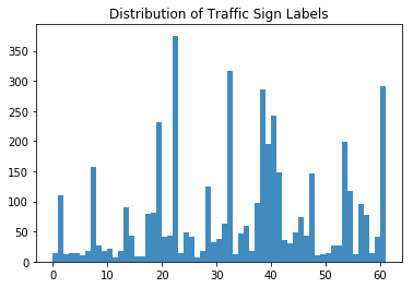
You clearly see that not all types of traffic signs are equally represented in the dataset. This is something that you’ll deal with later when you’re manipulating the data before you start modeling your neural network.
At first sight, you see that there are labels that are more heavily present in the dataset than others: the labels 22, 32, 38, and 61 definitely jump out. At this point, it’s nice to keep this in mind, but you’ll definitely go further into this in the next section\!
### Visualizing the Traffic Signs
The previous, small analyses or checks have already given you some idea of the data that you’re working with, but when your data mostly consists of images, the step that you should take to explore your data is by visualizing it.
Let’s check out some random traffic signs:
- First, make sure that you import the `pyplot` module of the `matplotlib` package under the common alias `plt`.
- Then, you’re going to make a list with 4 random numbers. These will be used to select traffic signs from the `images` array that you have just inspected in the previous section. In this case, you go for `300`, `2250`, `3650` and `4000`.
- Next, you’ll say that for every element in the length of that list, so from 0 to 4, you’re going to create subplots without axes (so that they don’t go running with all the attention and your focus is solely on the images!). In these subplots, you’re going to show a specific image from the `images` array that is in accordance with the number at the index `i`. In the first loop, you’ll pass `300` to `images[]`, in the second round `2250`, and so on. Lastly, you’ll adjust the subplots so that there’s enough width in between them.
- The last thing that remains is to show your plot with the help of the `show()` function\!
There you go:
```
Powered ByWas this AI assistant helpful? Yes No
```
As you guessed by the 62 labels that are included in this dataset, the signs are different from each other.
But what else do you notice? Take another close look at the images below:
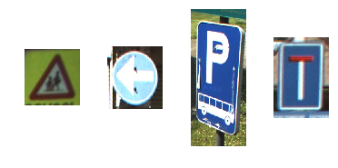
These four images are not of the same size\!
You can obviously toy around with the numbers that are contained in the `traffic_signs` list and follow up more thoroughly on this observation, but be as it may, this is an important observation which you will need to take into account when you start working more towards manipulating your data so that you can feed it to the neural network.
Let’s confirm the hypothesis of the differing sizes by printing the shape, the minimum and maximum values of the specific images that you have included into the subplots.
The code below heavily resembles the one that you used to create the above plot, but differs in the fact that here, you’ll alternate sizes and images instead of plotting just the images next to each other:
```
Powered ByWas this AI assistant helpful? Yes No
```
**Note** how you use the `format()` method on the string `"shape: {0}, min: {1}, max: {2}"` to fill out the arguments `{0}`, `{1}`, and `{2}` that you defined.
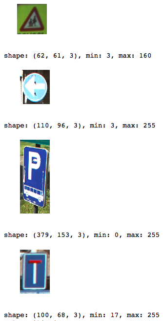
Now that you have seen loose images, you might also want to revisit the histogram that you printed out in the first steps of your data exploration; You can easily do this by plotting an overview of all the 62 classes and one image that belongs to each class:
```
Powered ByWas this AI assistant helpful? Yes No
```
**Note** that even though you define 64 subplots, not all of them will show images (as there are only 62 labels!). Note also that again, you don’t include any axes to make sure that the readers’ attention doesn’t dwell far from the main topic: the traffic signs\!
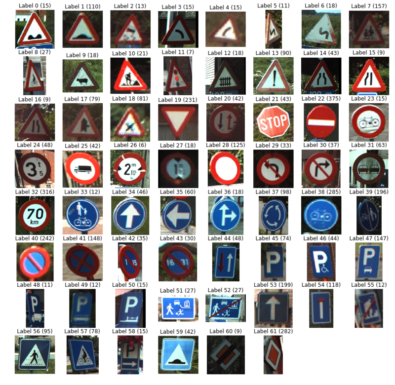
As you mostly guessed in the histogram above, there are considerably more traffic signs with labels 22, 32, 38, and 61. This hypothesis is now confirmed in this plot: you see that there are 375 instances with label 22, 316 instances with label 32, 285 instances with label 38 and, lastly, 282 instances with label 61.
One of the most interesting questions that you could ask yourself now is whether there’s a connection between all of these instances - maybe all of them are designatory signs?
Let’s take a closer look: you see that label 22 and 32 are prohibitory signs, but that labels 38 and 61 are designatory and a prioritory signs, respectively. This means that there’s not an immediate connection between these four, except for the fact that half of the signs that have a substantial presence in the dataset is of the prohibitory kind.
[](https://www.datacamp.com/learn/python)
## Feature Extraction
Now that you have thoroughly explored your data, it’s time to get your hands dirty! Let’s recap briefly what you discovered to make sure that you don’t forget any steps in the manipulation:
- The size of the images was unequal;
- There are 62 labels or target values (as your labels start at 0 and end at 61);
- The distribution of the traffic sign values is pretty unequal; There wasn’t really any connection between the signs that were heavily present in the dataset.
Now that you have a clear idea of what you need to improve, you can start with manipulating your data in such a way that it’s ready to be fed to the neural network or whichever model you want to feed it too. Let’s start first with extracting some features - you’ll rescale the images, and you’ll convert the images that are held in the `images` array to grayscale. You’ll do this color conversion mainly because the color matters less in classification questions like the one you’re trying to answer now. For detection, however, the color does play a big part! So in those cases, it’s not needed to do that conversion\!
#### Rescaling Images
To tackle the differing image sizes, you’re going to rescale the images; You can easily do this with the help of the `skimage` or Scikit-Image library, which is a collection of algorithms for image processing.
In this case, the `transform` module will come in handy, as it offers you a `resize()` function; You’ll see that you make use of list comprehension (again!) to resize each image to 28 by 28 pixels. Once again, you see that the way you actually form the list: for every image that you find in the `images` array, you’ll perform the transformation operation that you borrow from the `skimage` library. Finally, you store the result in the `images28` variable:
```
Powered ByWas this AI assistant helpful? Yes No
```
This was fairly easy wasn’t it?
**Note** that the images are now four-dimensional: if you convert `images28` to an array and if you concatenate the attribute `shape` to it, you’ll see that the printout tells you that `images28`’s dimensions are `(4575, 28, 28, 3)`. The images are 784-dimensional (because your images are 28 by 28 pixels).
You can check the result of the rescaling operation by re-using the code that you used above to plot the 4 random images with the help of the `traffic_signs` variable. Just don’t forget to change all references to `images` to `images28`.
Check out the result here:
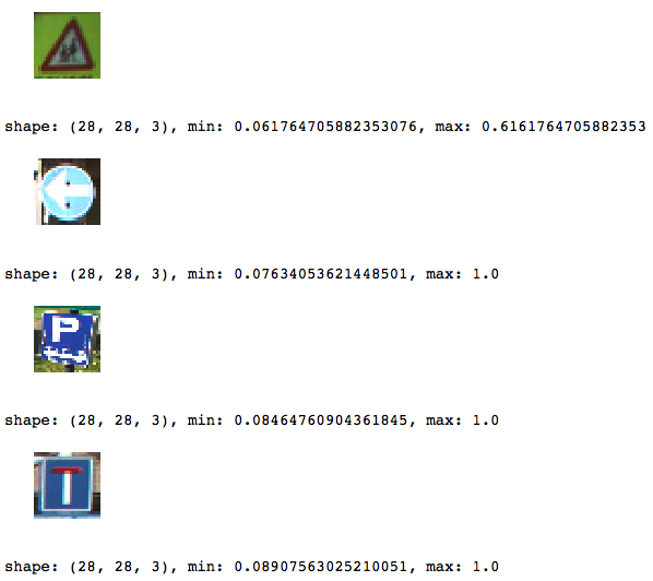
**Note** that because you rescaled, your `min` and `max` values have also changed; They seem to be all in the same ranges now, which is really great because then you don’t necessarily need to normalize your data\!
#### Image Conversion to Grayscale
As said in the introduction to this section of the tutorial, the color in the pictures matters less when you’re trying to answer a classification question. That’s why you’ll also go through the trouble of converting the images to grayscale.
**Note**, however, that you can also test out on your own what would happen to the final results of your model if you don’t follow through with this specific step.
Just like with the rescaling, you can again count on the Scikit-Image library to help you out; In this case, it’s the `color` module with its `rgb2gray()` function that you need to use to get where you need to be.
That’s going to be nice and easy\!
However, don’t forget to convert the `images28` variable back to an array, as the `rgb2gray()` function does expect an array as an argument.
```
Powered ByWas this AI assistant helpful? Yes No
```
Double check the result of your grayscale conversion by plotting some of the images; Here, you can again re-use and slightly adapt some of the code to show the adjusted images:
```
Powered ByWas this AI assistant helpful? Yes No
```
**Note** that you indeed have to specify the color map or `cmap` and set it to `"gray"` to plot the images in grayscale. That is because `imshow()` by default uses, by default, a heatmap-like color map. Read more [here](https://stackoverflow.com/questions/39805697/skimage-why-does-rgb2gray-from-skimage-color-result-in-a-colored-image).
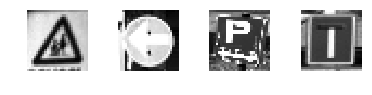
**Tip**: since you have been re-using this function quite a bit in this tutorial, you might look into how you can make it into a function :)
These two steps are very basic ones; Other operations that you could have tried out on your data include data augmentation (rotating, blurring, shifting, changing brightness,…). If you want, you could also set up an entire pipeline of data manipulation operations through which you send your images.
## Deep Learning with TensorFlow
Now that you have explored and manipulated your data, it’s time to construct your neural network architecture with the help of the TensorFlow package\!
### Modeling the Neural Network
Just like you might have done with Keras, it’s time to build up your neural network, layer by layer.
If you haven’t done so already, import `tensorflow` into your workspace under the conventional alias `tf`. Then, you can initialize the Graph with the help of `Graph()`. You use this function to define the computation. **Note** that with the Graph, you don’t compute anything, because it doesn’t hold any values. It just defines the operations that you want to be running later.
In this case, you set up a default context with the help of `as_default()`, which returns a context manager that makes this specific Graph the default graph. You use this method if you want to create multiple graphs in the same process: with this function, you have a global default graph to which all operations will be added if you don’t explicitly create a new graph.
Next, you’re ready to add operations to your graph. As you might remember from working with Keras, you build up your model, and then in compiling it, you define a loss function, an optimizer, and a metric. This now all happens in one step when you work with TensorFlow:
- - First, you define placeholders for inputs and labels because you won’t put in the “real” data yet. **Remember** that placeholders are values that are unassigned and that will be initialized by the session when you run it. So when you finally run the session, these placeholders will get the values of your dataset that you pass in the `run()` function\!
- Then, you build up the network. You first start by flattening the input with the help of the `flatten()` function, which will give you an array of shape `[None, 784]` instead of the `[None, 28, 28]`, which is the shape of your grayscale images.
- After you have flattened the input, you construct a fully connected layer that generates logits of size `[None, 62]`. Logits is the function operates on the unscaled output of previous layers, and that uses the relative scale to understand the units is linear.
- With the multi-layer perceptron built out, you can define the loss function. The choice for a loss function depends on the task that you have at hand: in this case, you make use of
```
sparse_softmax_cross_entropy_with_logits()Powered ByWas this AI assistant helpful? Yes No
```
- This computes sparse softmax cross entropy between logits and labels. In other words, it measures the probability error in discrete classification tasks in which the classes are mutually exclusive. This means that each entry is in exactly one class. Here, a traffic sign can only have one single label. **Remember** that, while regression is used to predict continuous values, classification is used to predict discrete values or classes of data points. You wrap this function with `reduce_mean()`, which computes the mean of elements across dimensions of a tensor.
- You also want to define a training optimizer; Some of the most popular optimization algorithms used are the Stochastic Gradient Descent (SGD), ADAM and RMSprop. Depending on whichever algorithm you choose, you’ll need to tune certain parameters, such as learning rate or momentum. In this case, you pick the ADAM optimizer, for which you define the learning rate at `0.001`.
- Lastly, you initialize the operations to execute before going over to the training.
```
Powered ByWas this AI assistant helpful? Yes No
```
You have now successfully created your first neural network with TensorFlow\!
If you want, you can also print out the values of (most of) the variables to get a quick recap or checkup of what you have just coded up:
```
Powered ByWas this AI assistant helpful? Yes No
```
**Tip**: if you see an error like “`module 'pandas' has no attribute 'computation'`”, consider upgrading the packages `dask` by running `pip install --upgrade dask` in your command line. See [this StackOverflow post](https://stackoverflow.com/questions/43833081/attributeerror-module-object-has-no-attribute-computation) for more information.
### Running the Neural Network
Now that you have built up your model layer by layer, it’s time to actually run it! To do this, you first need to initialize a session with the help of `Session()` to which you can pass your `graph` that you defined in the previous section. Next, you can run the session with `run()`, to which you pass the initialized operations in the form of the `init` variable that you also defined in the previous section.
Next, you can use this initialized session to start epochs or training loops. In this case, you pick `201` because you want to be able to register the last `loss_value`; In the loop, you run the session with the training optimizer and the loss (or accuracy) metric that you defined in the previous section. You also pass a `feed_dict` argument, with which you feed data to the model. After every 10 epochs, you’ll get a log that gives you more insights into the loss or cost of the model.
As you have seen in the section on the TensorFlow basics, there is no need to close the session manually; this is done for you. However, if you want to try out a different setup, you probably will need to do so with `sess.close()` if you have defined your session as `sess`, like in the code chunk below:
```
Powered ByWas this AI assistant helpful? Yes No
```
**Remember** that you can also run the following piece of code, but that one will immediately close the session afterward, just like you saw in the introduction of this tutorial:
```
Powered ByWas this AI assistant helpful? Yes No
```
**Note** that you make use of `global_variables_initializer()` because the `initialize_all_variables()` function is deprecated.
You have now successfully trained your model! That wasn’t too hard, was it?
### Evaluating your Neural Network
You’re not entirely there yet; You still need to evaluate your neural network. In this case, you can already try to get a glimpse of well your model performs by picking 10 random images and by comparing the predicted labels with the real labels.
You can first print them out, but why not use `matplotlib` to plot the traffic signs themselves and make a visual comparison?
```
Powered ByWas this AI assistant helpful? Yes No
```
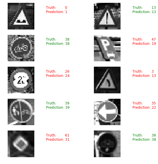
However, only looking at random images don’t give you many insights into how well your model actually performs. That’s why you’ll load in the test data.
**Note** that you make use of the `load_data()` function, which you defined at the start of this tutorial.
```
Powered ByWas this AI assistant helpful? Yes No
```
**Remember** to close off the session with `sess.close()` in case you didn't use the `with tf.Session() as sess:` to start your TensorFlow session.
## Where to Go Next?
If you want to continue working with this dataset and the model that you have put together in this tutorial, try out the following things:
- Apply regularized LDA on the data before you feed it to your model. This is a suggestion that comes from [one of the original papers](http://btsd.ethz.ch/shareddata/publications/Mathias-IJCNN-2013.pdf), written by the researchers that gathered and analyzed this dataset.
- You could also, as said in the tutorial itself, also look at some other data augmentation operations that you can perform on the traffic sign images. Additionally, you could also try to tweak this network further; The one that you have created now was fairly simple.
- Early stopping: Keep track of the training and testing error while you train the neural network. Stop training when both errors go down and then suddenly go back up - this is a sign that the neural network has started to overfit the training data.
- Play around with the optimizers.
Make sure to check out the [Machine Learning With TensorFlow](https://www.manning.com/books/machine-learning-with-tensorflow) book, written by Nishant Shukla.
**Tip** also check out the [TensorFlow Playground](http://playground.tensorflow.org/#activation=tanh&batchSize=10&dataset=circle®Dataset=reg-plane&learningRate=0.03®ularizationRate=0&noise=0&networkShape=4,2&seed=0.90110&showTestData=false&discretize=false&percTrainData=50&x=true&y=true&xTimesY=false&xSquared=false&ySquared=false&cosX=false&sinX=false&cosY=false&sinY=false&collectStats=false&problem=classification&initZero=false&hideText=false) and the [TensorBoard](https://www.tensorflow.org/get_started/summaries_and_tensorboard).
If you want to keep on working with images, definitely check out DataCamp’s [scikit-learn tutorial](https://www.datacamp.com/tutorial/machine-learning-python), which tackles the MNIST dataset with the help of [PCA](https://www.datacamp.com/tutorial/principal-component-analysis-in-python), K-Means and Support Vector Machines (SVMs). Or take a look at other tutorials such as [this one](https://github.com/waleedka/traffic-signs-tensorflow/blob/master/notebook1.ipynb) that uses the Belgian traffic signs dataset.
Topics
[Python](https://www.datacamp.com/tutorial/category/python)
[Artificial Intelligence](https://www.datacamp.com/tutorial/category/ai)
[Machine Learning](https://www.datacamp.com/tutorial/category/machine-learning)
[Deep Learning](https://www.datacamp.com/tutorial/category/deep-learning)
***
[Karlijn Willems](https://www.datacamp.com/portfolio/karlijn)Former Data Journalist at DataCamp \| Manager at NextWave Consulting
***
Topics
[Python](https://www.datacamp.com/tutorial/category/python)
[Artificial Intelligence](https://www.datacamp.com/tutorial/category/ai)
[Machine Learning](https://www.datacamp.com/tutorial/category/machine-learning)
[Deep Learning](https://www.datacamp.com/tutorial/category/deep-learning)

[Convolutional Neural Networks (CNN) with TensorFlow Tutorial](https://www.datacamp.com/tutorial/cnn-tensorflow-python)
[TensorBoard Tutorial](https://www.datacamp.com/tutorial/tensorboard-tutorial)
[Keras Tutorial: Deep Learning in Python](https://www.datacamp.com/tutorial/deep-learning-python)
[Investigating Tensors with PyTorch](https://www.datacamp.com/tutorial/investigating-tensors-pytorch)
[PyTorch CNN Tutorial: Build and Train Convolutional Neural Networks in Python](https://www.datacamp.com/tutorial/pytorch-cnn-tutorial)
[Metaflow Tutorial for Beginners: Build and Scale Data Workflows](https://www.datacamp.com/tutorial/metaflow)
Learn more about Python and Deep Learning
Course
### [Advanced Deep Learning with Keras](https://www.datacamp.com/courses/advanced-deep-learning-with-keras)
4 hr
34\.8K
Learn how to develop deep learning models with Keras.
[See Details](https://www.datacamp.com/courses/advanced-deep-learning-with-keras)
[Start Course](https://www.datacamp.com/users/sign_up?redirect=%2Fcourses%2Fadvanced-deep-learning-with-keras%2Fcontinue)
Course
### [Image Modeling with Keras](https://www.datacamp.com/courses/image-modeling-with-keras)
4 hr
39\.4K
Learn to conduct image analysis using Keras with Python by constructing, training, and evaluating convolutional neural networks.
[See Details](https://www.datacamp.com/courses/image-modeling-with-keras)
[Start Course](https://www.datacamp.com/users/sign_up?redirect=%2Fcourses%2Fimage-modeling-with-keras%2Fcontinue)
Course
### [Introduction to TensorFlow in Python](https://www.datacamp.com/courses/introduction-to-tensorflow-in-python)
4 hr
55\.8K
Learn the fundamentals of neural networks and how to build deep learning models using TensorFlow.
[See Details](https://www.datacamp.com/courses/introduction-to-tensorflow-in-python)
[Start Course](https://www.datacamp.com/users/sign_up?redirect=%2Fcourses%2Fintroduction-to-tensorflow-in-python%2Fcontinue)
[See More](https://www.datacamp.com/category/python)
Related
[TutorialConvolutional Neural Networks (CNN) with TensorFlow Tutorial](https://www.datacamp.com/tutorial/cnn-tensorflow-python)
Learn how to construct and implement Convolutional Neural Networks (CNNs) in Python with Tensorflow Framework 2
[](https://www.datacamp.com/portfolio/keitazoumana)
Zoumana Keita
[TutorialTensorBoard Tutorial](https://www.datacamp.com/tutorial/tensorboard-tutorial)
Visualize the training parameters, metrics, hyperparameters or any statistics of your neural network with TensorBoard\!
[](https://www.datacamp.com/portfolio/thushv)
Thushan Ganegedara
[TutorialKeras Tutorial: Deep Learning in Python](https://www.datacamp.com/tutorial/deep-learning-python)
This Keras tutorial introduces you to deep learning in Python: learn to preprocess your data, model, evaluate and optimize neural networks.
[](https://www.datacamp.com/portfolio/karlijn)
Karlijn Willems
[TutorialInvestigating Tensors with PyTorch](https://www.datacamp.com/tutorial/investigating-tensors-pytorch)
In this tutorial, you'll learn about Tensors, PyTorch, and how to create a simple neural network with PyTorch.
[](https://www.datacamp.com/portfolio/spsayakpaul)
Sayak Paul
[TutorialPyTorch CNN Tutorial: Build and Train Convolutional Neural Networks in Python](https://www.datacamp.com/tutorial/pytorch-cnn-tutorial)
Learn how to construct and implement Convolutional Neural Networks (CNNs) in Python with PyTorch.
[](https://www.datacamp.com/portfolio/jcanalesluna)
Javier Canales Luna
[TutorialMetaflow Tutorial for Beginners: Build and Scale Data Workflows](https://www.datacamp.com/tutorial/metaflow)
This beginner-friendly tutorial will guide you through the fundamentals of Metaflow. Learn how the framework simplifies building and scaling data science workflows.
[](https://www.datacamp.com/portfolio/kurtispykes)
Kurtis Pykes
[See More](https://www.datacamp.com/tutorial/category/python)
[See More](https://www.datacamp.com/tutorial/category/python)
## Grow your data skills with DataCamp for Mobile
Make progress on the go with our mobile courses and daily 5-minute coding challenges.
[Download on the App Store](https://datacamp.onelink.me/xztQ/45dozwue?deep_link_sub1=%7B%22src_url%22%3A%22https%3A%2F%2Fwww.datacamp.com%2Ftutorial%2Ftensorflow-tutorial%22%7D)[Get it on Google Play](https://datacamp.onelink.me/xztQ/go2f19ij?deep_link_sub1=%7B%22src_url%22%3A%22https%3A%2F%2Fwww.datacamp.com%2Ftutorial%2Ftensorflow-tutorial%22%7D)
**Learn**
[Learn Python](https://www.datacamp.com/blog/how-to-learn-python-expert-guide)[Learn AI](https://www.datacamp.com/blog/how-to-learn-ai)[Learn Power BI](https://www.datacamp.com/learn/power-bi)[Learn Data Engineering](https://www.datacamp.com/category/data-engineering)[Assessments](https://www.datacamp.com/signal)[Career Tracks](https://www.datacamp.com/tracks/career)[Skill Tracks](https://www.datacamp.com/tracks/skill)[Courses](https://www.datacamp.com/courses-all)[Data Science Roadmap](https://www.datacamp.com/blog/data-science-roadmap)
**Data Courses**
[Python Courses](https://www.datacamp.com/category/python)[R Courses](https://www.datacamp.com/category/r)[SQL Courses](https://www.datacamp.com/category/sql)[Power BI Courses](https://www.datacamp.com/category/power-bi)[Tableau Courses](https://www.datacamp.com/category/tableau)[Alteryx Courses](https://www.datacamp.com/category/alteryx)[Azure Courses](https://www.datacamp.com/category/azure)[AWS Courses](https://www.datacamp.com/category/aws)[Google Cloud Courses](https://www.datacamp.com/category/google-cloud)[Google Sheets Courses](https://www.datacamp.com/category/google-sheets)[Excel Courses](https://www.datacamp.com/category/excel)[AI Courses](https://www.datacamp.com/category/artificial-intelligence)[Data Analysis Courses](https://www.datacamp.com/category/data-analysis)[Data Visualization Courses](https://www.datacamp.com/category/data-visualization)[Machine Learning Courses](https://www.datacamp.com/category/machine-learning)[Data Engineering Courses](https://www.datacamp.com/category/data-engineering)[Probability & Statistics Courses](https://www.datacamp.com/category/probability-and-statistics)
**DataLab**
[Get Started](https://www.datacamp.com/datalab)[Pricing](https://www.datacamp.com/datalab/pricing)[Security](https://www.datacamp.com/datalab/security)[Documentation](https://datalab-docs.datacamp.com/)
**Certification**
[Certifications](https://www.datacamp.com/certification)[Data Scientist](https://www.datacamp.com/certification/data-scientist)[Data Analyst](https://www.datacamp.com/certification/data-analyst)[Data Engineer](https://www.datacamp.com/certification/data-engineer)[SQL Associate](https://www.datacamp.com/certification/sql-associate)[Power BI Data Analyst](https://www.datacamp.com/certification/data-analyst-in-power-bi)[Tableau Certified Data Analyst](https://www.datacamp.com/certification/data-analyst-in-tableau)[Azure Fundamentals](https://www.datacamp.com/certification/azure-fundamentals)[AI Fundamentals](https://www.datacamp.com/certification/ai-fundamentals)
**Resources**
[Resource Center](https://www.datacamp.com/resources)[Upcoming Events](https://www.datacamp.com/webinars)[Blog](https://www.datacamp.com/blog)[Code-Alongs](https://www.datacamp.com/code-along)[Tutorials](https://www.datacamp.com/tutorial)[Docs](https://www.datacamp.com/doc)[Open Source](https://www.datacamp.com/open-source)[RDocumentation](https://www.rdocumentation.org/)[Book a Demo with DataCamp for Business](https://www.datacamp.com/business/demo)[Data Portfolio](https://www.datacamp.com/data-portfolio)
**Plans**
[Pricing](https://www.datacamp.com/pricing)[For Students](https://www.datacamp.com/pricing/student)[For Business](https://www.datacamp.com/business)[For Universities](https://www.datacamp.com/universities)[Discounts, Promos & Sales](https://www.datacamp.com/promo)[Expense DataCamp](https://www.datacamp.com/expense)[DataCamp Donates](https://www.datacamp.com/donates)
**For Business**
[Business Pricing](https://www.datacamp.com/business/compare-plans)[Teams Plan](https://www.datacamp.com/business/learn-teams)[Data & AI Unlimited Plan](https://www.datacamp.com/business/data-unlimited)[Customer Stories](https://www.datacamp.com/business/customer-stories)[Partner Program](https://www.datacamp.com/business/partner-program)
**About**
[About Us](https://www.datacamp.com/about)[Learner Stories](https://www.datacamp.com/stories)[Careers](https://www.datacamp.com/careers)[Become an Instructor](https://www.datacamp.com/learn/create)[Press](https://www.datacamp.com/press)[Leadership](https://www.datacamp.com/about/leadership)[Contact Us](https://support.datacamp.com/hc/en-us/articles/360021185634)[DataCamp Español](https://www.datacamp.com/es)[DataCamp Português](https://www.datacamp.com/pt)[DataCamp Deutsch](https://www.datacamp.com/de)[DataCamp Français](https://www.datacamp.com/fr)
**Support**
[Help Center](https://support.datacamp.com/hc/en-us)[Become an Affiliate](https://www.datacamp.com/affiliates)
[Facebook](https://www.facebook.com/datacampinc/)
[Twitter](https://twitter.com/datacamp)
[LinkedIn](https://www.linkedin.com/school/datacampinc/)
[YouTube](https://www.youtube.com/channel/UC79Gv3mYp6zKiSwYemEik9A)
[Instagram](https://www.instagram.com/datacamp/)
[Privacy Policy](https://www.datacamp.com/privacy-policy)[Cookie Notice](https://www.datacamp.com/cookie-notice)[Do Not Sell My Personal Information](https://www.datacamp.com/do-not-sell-my-personal-information)[Accessibility](https://www.datacamp.com/accessibility)[Security](https://www.datacamp.com/security)[Terms of Use](https://www.datacamp.com/terms-of-use)
© 2026 DataCamp, Inc. All Rights Reserved. | ||||||||||||||||||
| Readable Markdown |  Deep learning is a subfield of machine learning that is a set of algorithms that is inspired by the structure and function of the brain. TensorFlow is the second machine learning framework that Google created and used to design, build, and train deep learning models. You can use the TensorFlow library do to numerical computations, which in itself doesn’t seem all too special, but these computations are done with data flow graphs. In these graphs, nodes represent mathematical operations, while the edges represent the data, which usually are multidimensional data arrays or tensors, that are communicated between these edges. You see? The name “TensorFlow” is derived from the operations which neural networks perform on multidimensional data arrays or tensors! It’s literally a flow of tensors. For now, this is all you need to know about tensors, but you’ll go deeper into this in the next sections\! Today’s TensorFlow tutorial for beginners will introduce you to performing deep learning in an interactive way: You’ll first learn more about [tensors](https://www.datacamp.com/tutorial/tensorflow-tutorial#introducing-tensors); Then, the tutorial you’ll briefly go over some of the ways that you can [install TensorFlow](https://www.datacamp.com/tutorial/tensorflow-tutorial#installing-tensorflow) on your system so that you’re able to get started and load data in your workspace; After this, you’ll go over some of the [TensorFlow basics](https://www.datacamp.com/tutorial/tensorflow-tutorial#getting-started-with-tensorflow:-basics): you’ll see how you can easily get started with simple computations. After this, you get started on the real work: you’ll load in data on [Belgian traffic signs](https://www.datacamp.com/tutorial/tensorflow-tutorial#belgian-traffic-signs:-background) and [exploring](https://www.datacamp.com/tutorial/tensorflow-tutorial#loading-and-exploring-the-data) it with simple statistics and plotting. In your exploration, you’ll see that there is a need to [manipulate your data](https://www.datacamp.com/tutorial/tensorflow-tutorial#feature-extraction) in such a way that you can feed it to your model. That’s why you’ll take the time to rescale your images and convert them to grayscale. Next, you can finally get started on [your neural network model](https://www.datacamp.com/tutorial/tensorflow-tutorial#deep-learning-with-tensorflow)! You’ll build up your model layer per layer; Once the architecture is set up, you can use it to [train your model interactively](https://www.datacamp.com/tutorial/tensorflow-tutorial#running-the-neural-network) and to eventually also [evaluate](https://www.datacamp.com/tutorial/tensorflow-tutorial#evaluating-your-neural-network) it by feeding some test data to it. Lastly, you’ll get some pointers for [further](https://www.datacamp.com/tutorial/tensorflow-tutorial#where-to-go-next?) improvements that you can do to the model you just constructed and how you can continue your learning with TensorFlow. Download the notebook of this tutorial [here](https://github.com/datacamp/datacamp-community-tutorials). Also, you could be interested in a course on [Deep Learning in Python](https://www.datacamp.com/courses/deep-learning-in-python), DataCamp's [Keras tutorial](https://www.datacamp.com/tutorial/deep-learning-python) or the [keras with R tutorial](https://www.datacamp.com/tutorial/keras-r-deep-learning). Introducing Tensors To understand tensors well, it’s good to have some working knowledge of linear algebra and vector calculus. You already read in the introduction that tensors are implemented in TensorFlow as multidimensional data arrays, but some more introduction is maybe needed in order to completely grasp tensors and their use in machine learning. Plane Vectors Before you go into plane vectors, it’s a good idea to shortly revise the concept of “vectors”; Vectors are special types of matrices, which are rectangular arrays of numbers. Because vectors are ordered collections of numbers, they are often seen as column matrices: they have just one column and a certain number of rows. In other terms, you could also consider vectors as scalar magnitudes that have been given a direction. **Remember**: an example of a scalar is “5 meters” or “60 m/sec”, while a vector is, for example, “5 meters north” or “60 m/sec East”. The difference between these two is obviously that the vector has a direction. Nevertheless, these examples that you have seen up until now might seem far off from the vectors that you might encounter when you’re working with machine learning problems. This is normal; The length of a mathematical vector is a pure number: it is absolute. The direction, on the other hand, is relative: it is measured relative to some reference direction and has units of radians or degrees. You usually assume that the direction is positive and in counterclockwise rotation from the reference direction.  Visually, of course, you represent vectors as arrows, as you can see in the picture above. This means that you can consider vectors also as arrows that have direction and length. The direction is indicated by the arrow’s head, while the length is indicated by the length of the arrow. So what about plane vectors then? Plane vectors are the most straightforward setup of tensors. They are much like regular vectors as you have seen above, with the sole difference that they find themselves in a vector space. To understand this better, let’s start with an example: you have a vector that is *2 X 1*. This means that the vector belongs to the set of real numbers that come paired two at a time. Or, stated differently, they are part of two-space. In such cases, you can represent vectors on the coordinate *(x,y)* plane with arrows or rays. Working from this coordinate plane in a standard position where vectors have their endpoint at the origin *(0,0)*, you can derive the *x* coordinate by looking at the first row of the vector, while you’ll find the *y* coordinate in the second row. Of course, this standard position doesn’t always need to be maintained: vectors can move parallel to themselves in the plane without experiencing changes. **Note** that similarly, for vectors that are of size *3 X 1*, you talk about the three-space. You can represent the vector as a three-dimensional figure with arrows pointing to positions in the vectors pace: they are drawn on the standard *x*, *y* and *z* axes. It’s nice to have these vectors and to represent them on the coordinate plane, but in essence, you have these vectors so that you can perform operations on them and one thing that can help you in doing this is by expressing your vectors as bases or unit vectors. Unit vectors are vectors with a magnitude of one. You’ll often recognize the unit vector by a lowercase letter with a circumflex, or “hat”. Unit vectors will come in convenient if you want to express a 2-D or 3-D vector as a sum of two or three orthogonal components, such as the x− and y−axes, or the z−axis. And when you are talking about expressing one vector, for example, as sums of components, you’ll see that you’re talking about component vectors, which are two or more vectors whose sum is that given vector. **Tip**: watch [this video](https://www.youtube.com/watch?v=f5liqUk0ZTw), which explains what tensors are with the help of simple household objects\! Tensors Next to plane vectors, also covectors and linear operators are two other cases that all three together have one thing in common: they are specific cases of tensors. You still remember how a vector was characterized in the previous section as scalar magnitudes that have been given a direction. A tensor, then, is the mathematical representation of a physical entity that may be characterized by magnitude and *multiple* directions. And, just like you represent a scalar with a single number and a vector with a sequence of three numbers in a 3-dimensional space, for example, a tensor can be represented by an array of 3R numbers in a 3-dimensional space. The “R” in this notation represents the rank of the tensor: this means that in a 3-dimensional space, a second-rank tensor can be represented by 3 to the power of 2 or 9 numbers. In an N-dimensional space, scalars will still require only one number, while vectors will require N numbers, and tensors will require N^R numbers. This explains why you often hear that scalars are tensors of rank 0: since they have no direction, you can represent them with one number. With this in mind, it’s relatively easy to recognize scalars, vectors, and tensors and to set them apart: scalars can be represented by a single number, vectors by an ordered set of numbers, and tensors by an array of numbers. What makes tensors so unique is the combination of components and basis vectors: basis vectors transform one way between reference frames and the components transform in just such a way as to keep the combination between components and basis vectors the same. Installing TensorFlow Now that you know more about TensorFlow, it’s time to get started and install the library. Here, it’s good to know that TensorFlow provides APIs for Python, C++, Haskell, Java, Go, Rust, and there’s also a third-party package for R called `tensorflow`. **Tip**: if you want to know more about deep learning packages in R, consider checking out DataCamp’s [keras: Deep Learning in R Tutorial](https://www.datacamp.com/tutorial/keras-r-deep-learning). In this tutorial, you will download a version of TensorFlow that will enable you to write the code for your deep learning project in Python. On the [TensorFlow installation webpage](https://www.tensorflow.org/install), you’ll see some of the most common ways and latest instructions to install TensorFlow using `virtualenv`, `pip`, Docker and lastly, there are also some of the other ways of installing TensorFlow on your personal computer. **Note** You can also install TensorFlow with Conda if you’re working on Windows. However, since the installation of TensorFlow is community supported, it’s best to check the [official installation instructions](https://www.tensorflow.org/install/install_windows). Now that you have gone through the installation process, it’s time to double check that you have installed TensorFlow correctly by importing it into your workspace under the alias `tf`: **Note** that the alias that you used in the line of code above is sort of a convention - It’s used to ensure that you remain consistent with other developers that are using TensorFlow in data science projects on the one hand, and with open-source TensorFlow projects on the other hand. Getting Started with TensorFlow: Basics You’ll generally write TensorFlow programs, which you run as a chunk; This is at first sight kind of contradictory when you’re working with Python. However, if you would like, you can also use TensorFlow’s Interactive Session, which you can use to work more interactively with the library. This is especially handy when you’re used to working with IPython. For this tutorial, you’ll focus on the second option: this will help you to get kickstarted with deep learning in TensorFlow. But before you go any further into this, let’s first try out some minor stuff before you start with the heavy lifting. First, import the `tensorflow` library under the alias `tf`, as you have seen in the previous section. Then initialize two variables that are actually constants. Pass an array of four numbers to the `constant()` function. **Note** that you could potentially also pass in an integer, but that more often than not, you’ll find yourself working with arrays. As you saw in the introduction, tensors are all about arrays! So make sure that you pass in an array :) Next, you can use `multiply()` to multiply your two variables. Store the result in the `result` variable. Lastly, print out the `result` with the help of the `print()` function. script.py 7 IPython Shell **Note** that you have defined constants in the DataCamp Light code chunk above. However, there are two other types of values that you can potentially use, namely [placeholders](https://www.tensorflow.org/api_docs/python/tf/placeholder), which are values that are unassigned and that will be initialized by the session when you run it. Like the name already gave away, it’s just a placeholder for a tensor that will always be fed when the session is run; There are also [Variables](https://www.tensorflow.org/api_docs/python/tf/Variable), which are values that can change. The constants, as you might have already gathered, are values that don’t change. The result of the lines of code is an abstract tensor in the computation graph. However, contrary to what you might expect, the `result` doesn’t actually get calculated. It just defined the model, but no process ran to calculate the result. You can see this in the print-out: there’s not really a result that you want to see (namely, 30). This means that TensorFlow has a lazy evaluation\! However, if you do want to see the result, you have to run this code in an interactive session. You can do this in a few ways, as is demonstrated in the DataCamp Light code chunks below: script.py 10 IPython Shell **Note** that you can also use the following lines of code to start up an interactive Session, run the `result` and close the Session automatically again after printing the `output`: script.py 8 IPython Shell In the code chunks above you have just defined a default Session, but it’s also good to know that you can pass in options as well. You can, for example, specify the `config` argument and then use the `ConfigProto` protocol buffer to add configuration options for your session. For example, if you add to your Session, you make sure that you log the GPU or CPU device that is assigned to an operation. You will then get information which devices are used in the session for each operation. You could use the following configuration session also, for example, when you use soft constraints for the device placement: Now that you’ve got TensorFlow installed and imported into your workspace and you’ve gone through the basics of working with this package, it’s time to leave this aside for a moment and turn your attention to your data. Just like always, you’ll first take your time to explore and understand your data better before you start modeling your neural network. Belgian Traffic Signs: Background Even though traffic is a topic that is generally known amongst you all, it doesn’t hurt going briefly over the observations that are included in this dataset to see if you understand everything before you start. In essence, in this section, you’ll get up to speed with the domain knowledge that you need to have to go further with this tutorial. Of course, because I’m Belgian, I’ll make sure you’ll also get some anecdotes :) Belgian traffic signs are usually in Dutch and French. This is good to know, but for the dataset that you’ll be working with, it’s not too important\! There are six categories of traffic signs in Belgium: warning signs, priority signs, prohibitory signs, mandatory signs, signs related to parking and standing still on the road and, lastly, designatory signs. On January 1st, 2017, more than 30,000 traffic signs were removed from Belgian roads. These were all prohibitory signs relating to speed. Talking about removal, the overwhelming presence of traffic signs has been an ongoing discussion in Belgium (and by extension, the entire European Union). Loading and Exploring the Data Now that you have gathered some more background information, it’s time to download the dataset [here](http://btsd.ethz.ch/shareddata). You should get the two zip files listed next to "BelgiumTS for Classification (cropped images), which are called "BelgiumTSC\_Training" and "BelgiumTSC\_Testing". **Tip**: if you have downloaded the files or will do so after completing this tutorial, take a look at the folder structure of the data that you’ve downloaded! You’ll see that the testing, as well as the training data folders, contain 61 subfolders, which are the 62 types of traffic signs that you’ll use for classification in this tutorial. Additionally, you’ll find that the files have the file extension `.ppm` or Portable Pixmap Format. You have downloaded images of the traffic signs\! Let’s get started with importing the data into your workspace. Let’s start with the lines of code that appear below the User-Defined Function (UDF) `load_data()`: First, set your `ROOT_PATH`. This path is the one where you have made the directory with your training and test data. Next, you can add the specific paths to your `ROOT_PATH` with the help of the `join()` function. You store these two specific paths in `train_data_directory` and `test_data_directory`. You see that after, you can call the `load_data()` function and pass in the `train_data_directory` to it. Now, the `load_data()` function itself starts off by gathering all the subdirectories that are present in the `train_data_directory`; It does so with the help of list comprehension, which is quite a natural way of constructing lists - it basically says that, if you find something in the `train_data_directory`, you’ll double check whether this is a directory, and if it is one, you’ll add it to your list. **Remember** that each subdirectory represents a label. Next, you have to loop through the subdirectories. You first initialize two lists, `labels` and `images`. Next, you gather the paths of the subdirectories and the file names of the images that are stored in these subdirectories. After, you can collect the data in the two lists with the help of the `append()` function. **Note** that in the above code chunk, the training and test data are located in folders named "Training" and "Testing", which are both subdirectories of another directory "TrafficSigns". On a local machine, this could look something like "/Users/Name/Downloads/TrafficSigns", with then two subfolders called "Training" and "Testing". **Tip**: review how to write functions in Python with DataCamp's [Python Functions Tutorial](https://www.datacamp.com/tutorial/functions-python-tutorial). Traffic Sign Statistics With your data loaded in, it’s time for some data inspection! You can start with a pretty simple analysis with the help of the `ndim` and `size` attributes of the `images` array: Note that the `images` and `labels` variables are lists, so you might need to use `np.array()` to convert the variables to an array in your own workspace. This has been done for you here\! script.py 5 IPython Shell **Note** that the `images[0]` that you printed out is, in fact, one single image that is represented by arrays in arrays! This might seem counterintuitive at first, but it’s something that you’ll get used to as you go further into working with images in machine learning or deep learning applications. Next, you can also take a small look at the `labels`, but you shouldn’t see too many surprises at this point: script.py 5 IPython Shell These numbers already give you some insights into how successful your import was and the exact size of your data. At first sight, everything has been executed the way you expected it to, and you see that the size of the array is considerable if you take into account that you’re dealing with arrays within arrays. **Tip** try adding the following attributes to your arrays to get more information about the memory layout, the length of one array element in bytes and the total consumed bytes by the array’s elements with the `flags`, `itemsize`, and `nbytes` attributes. You can test this out in the IPython console in the DataCamp Light chunk above\! Next, you can also take a look at the distribution of the traffic signs: script.py 5 IPython Shell Awesome job! Now let’s take a closer look at the histogram that you made\!  You clearly see that not all types of traffic signs are equally represented in the dataset. This is something that you’ll deal with later when you’re manipulating the data before you start modeling your neural network. At first sight, you see that there are labels that are more heavily present in the dataset than others: the labels 22, 32, 38, and 61 definitely jump out. At this point, it’s nice to keep this in mind, but you’ll definitely go further into this in the next section\! Visualizing the Traffic Signs The previous, small analyses or checks have already given you some idea of the data that you’re working with, but when your data mostly consists of images, the step that you should take to explore your data is by visualizing it. Let’s check out some random traffic signs: First, make sure that you import the `pyplot` module of the `matplotlib` package under the common alias `plt`. Then, you’re going to make a list with 4 random numbers. These will be used to select traffic signs from the `images` array that you have just inspected in the previous section. In this case, you go for `300`, `2250`, `3650` and `4000`. Next, you’ll say that for every element in the length of that list, so from 0 to 4, you’re going to create subplots without axes (so that they don’t go running with all the attention and your focus is solely on the images!). In these subplots, you’re going to show a specific image from the `images` array that is in accordance with the number at the index `i`. In the first loop, you’ll pass `300` to `images[]`, in the second round `2250`, and so on. Lastly, you’ll adjust the subplots so that there’s enough width in between them. The last thing that remains is to show your plot with the help of the `show()` function\! There you go: As you guessed by the 62 labels that are included in this dataset, the signs are different from each other. But what else do you notice? Take another close look at the images below:  These four images are not of the same size\! You can obviously toy around with the numbers that are contained in the `traffic_signs` list and follow up more thoroughly on this observation, but be as it may, this is an important observation which you will need to take into account when you start working more towards manipulating your data so that you can feed it to the neural network. Let’s confirm the hypothesis of the differing sizes by printing the shape, the minimum and maximum values of the specific images that you have included into the subplots. The code below heavily resembles the one that you used to create the above plot, but differs in the fact that here, you’ll alternate sizes and images instead of plotting just the images next to each other: **Note** how you use the `format()` method on the string `"shape: {0}, min: {1}, max: {2}"` to fill out the arguments `{0}`, `{1}`, and `{2}` that you defined.  Now that you have seen loose images, you might also want to revisit the histogram that you printed out in the first steps of your data exploration; You can easily do this by plotting an overview of all the 62 classes and one image that belongs to each class: **Note** that even though you define 64 subplots, not all of them will show images (as there are only 62 labels!). Note also that again, you don’t include any axes to make sure that the readers’ attention doesn’t dwell far from the main topic: the traffic signs\!  As you mostly guessed in the histogram above, there are considerably more traffic signs with labels 22, 32, 38, and 61. This hypothesis is now confirmed in this plot: you see that there are 375 instances with label 22, 316 instances with label 32, 285 instances with label 38 and, lastly, 282 instances with label 61. One of the most interesting questions that you could ask yourself now is whether there’s a connection between all of these instances - maybe all of them are designatory signs? Let’s take a closer look: you see that label 22 and 32 are prohibitory signs, but that labels 38 and 61 are designatory and a prioritory signs, respectively. This means that there’s not an immediate connection between these four, except for the fact that half of the signs that have a substantial presence in the dataset is of the prohibitory kind. [](https://www.datacamp.com/learn/python) Feature Extraction Now that you have thoroughly explored your data, it’s time to get your hands dirty! Let’s recap briefly what you discovered to make sure that you don’t forget any steps in the manipulation: The size of the images was unequal; There are 62 labels or target values (as your labels start at 0 and end at 61); The distribution of the traffic sign values is pretty unequal; There wasn’t really any connection between the signs that were heavily present in the dataset. Now that you have a clear idea of what you need to improve, you can start with manipulating your data in such a way that it’s ready to be fed to the neural network or whichever model you want to feed it too. Let’s start first with extracting some features - you’ll rescale the images, and you’ll convert the images that are held in the `images` array to grayscale. You’ll do this color conversion mainly because the color matters less in classification questions like the one you’re trying to answer now. For detection, however, the color does play a big part! So in those cases, it’s not needed to do that conversion\! Rescaling Images To tackle the differing image sizes, you’re going to rescale the images; You can easily do this with the help of the `skimage` or Scikit-Image library, which is a collection of algorithms for image processing. In this case, the `transform` module will come in handy, as it offers you a `resize()` function; You’ll see that you make use of list comprehension (again!) to resize each image to 28 by 28 pixels. Once again, you see that the way you actually form the list: for every image that you find in the `images` array, you’ll perform the transformation operation that you borrow from the `skimage` library. Finally, you store the result in the `images28` variable: This was fairly easy wasn’t it? **Note** that the images are now four-dimensional: if you convert `images28` to an array and if you concatenate the attribute `shape` to it, you’ll see that the printout tells you that `images28`’s dimensions are `(4575, 28, 28, 3)`. The images are 784-dimensional (because your images are 28 by 28 pixels). You can check the result of the rescaling operation by re-using the code that you used above to plot the 4 random images with the help of the `traffic_signs` variable. Just don’t forget to change all references to `images` to `images28`. Check out the result here:  **Note** that because you rescaled, your `min` and `max` values have also changed; They seem to be all in the same ranges now, which is really great because then you don’t necessarily need to normalize your data\! Image Conversion to Grayscale As said in the introduction to this section of the tutorial, the color in the pictures matters less when you’re trying to answer a classification question. That’s why you’ll also go through the trouble of converting the images to grayscale. **Note**, however, that you can also test out on your own what would happen to the final results of your model if you don’t follow through with this specific step. Just like with the rescaling, you can again count on the Scikit-Image library to help you out; In this case, it’s the `color` module with its `rgb2gray()` function that you need to use to get where you need to be. That’s going to be nice and easy\! However, don’t forget to convert the `images28` variable back to an array, as the `rgb2gray()` function does expect an array as an argument. Double check the result of your grayscale conversion by plotting some of the images; Here, you can again re-use and slightly adapt some of the code to show the adjusted images: **Note** that you indeed have to specify the color map or `cmap` and set it to `"gray"` to plot the images in grayscale. That is because `imshow()` by default uses, by default, a heatmap-like color map. Read more [here](https://stackoverflow.com/questions/39805697/skimage-why-does-rgb2gray-from-skimage-color-result-in-a-colored-image).  **Tip**: since you have been re-using this function quite a bit in this tutorial, you might look into how you can make it into a function :) These two steps are very basic ones; Other operations that you could have tried out on your data include data augmentation (rotating, blurring, shifting, changing brightness,…). If you want, you could also set up an entire pipeline of data manipulation operations through which you send your images. Deep Learning with TensorFlow Now that you have explored and manipulated your data, it’s time to construct your neural network architecture with the help of the TensorFlow package\! Modeling the Neural Network Just like you might have done with Keras, it’s time to build up your neural network, layer by layer. If you haven’t done so already, import `tensorflow` into your workspace under the conventional alias `tf`. Then, you can initialize the Graph with the help of `Graph()`. You use this function to define the computation. **Note** that with the Graph, you don’t compute anything, because it doesn’t hold any values. It just defines the operations that you want to be running later. In this case, you set up a default context with the help of `as_default()`, which returns a context manager that makes this specific Graph the default graph. You use this method if you want to create multiple graphs in the same process: with this function, you have a global default graph to which all operations will be added if you don’t explicitly create a new graph. Next, you’re ready to add operations to your graph. As you might remember from working with Keras, you build up your model, and then in compiling it, you define a loss function, an optimizer, and a metric. This now all happens in one step when you work with TensorFlow: First, you define placeholders for inputs and labels because you won’t put in the “real” data yet. **Remember** that placeholders are values that are unassigned and that will be initialized by the session when you run it. So when you finally run the session, these placeholders will get the values of your dataset that you pass in the `run()` function\! Then, you build up the network. You first start by flattening the input with the help of the `flatten()` function, which will give you an array of shape `[None, 784]` instead of the `[None, 28, 28]`, which is the shape of your grayscale images. After you have flattened the input, you construct a fully connected layer that generates logits of size `[None, 62]`. Logits is the function operates on the unscaled output of previous layers, and that uses the relative scale to understand the units is linear. With the multi-layer perceptron built out, you can define the loss function. The choice for a loss function depends on the task that you have at hand: in this case, you make use of This computes sparse softmax cross entropy between logits and labels. In other words, it measures the probability error in discrete classification tasks in which the classes are mutually exclusive. This means that each entry is in exactly one class. Here, a traffic sign can only have one single label. **Remember** that, while regression is used to predict continuous values, classification is used to predict discrete values or classes of data points. You wrap this function with `reduce_mean()`, which computes the mean of elements across dimensions of a tensor. You also want to define a training optimizer; Some of the most popular optimization algorithms used are the Stochastic Gradient Descent (SGD), ADAM and RMSprop. Depending on whichever algorithm you choose, you’ll need to tune certain parameters, such as learning rate or momentum. In this case, you pick the ADAM optimizer, for which you define the learning rate at `0.001`. Lastly, you initialize the operations to execute before going over to the training. You have now successfully created your first neural network with TensorFlow\! If you want, you can also print out the values of (most of) the variables to get a quick recap or checkup of what you have just coded up: **Tip**: if you see an error like “`module 'pandas' has no attribute 'computation'`”, consider upgrading the packages `dask` by running `pip install --upgrade dask` in your command line. See [this StackOverflow post](https://stackoverflow.com/questions/43833081/attributeerror-module-object-has-no-attribute-computation) for more information. Running the Neural Network Now that you have built up your model layer by layer, it’s time to actually run it! To do this, you first need to initialize a session with the help of `Session()` to which you can pass your `graph` that you defined in the previous section. Next, you can run the session with `run()`, to which you pass the initialized operations in the form of the `init` variable that you also defined in the previous section. Next, you can use this initialized session to start epochs or training loops. In this case, you pick `201` because you want to be able to register the last `loss_value`; In the loop, you run the session with the training optimizer and the loss (or accuracy) metric that you defined in the previous section. You also pass a `feed_dict` argument, with which you feed data to the model. After every 10 epochs, you’ll get a log that gives you more insights into the loss or cost of the model. As you have seen in the section on the TensorFlow basics, there is no need to close the session manually; this is done for you. However, if you want to try out a different setup, you probably will need to do so with `sess.close()` if you have defined your session as `sess`, like in the code chunk below: **Remember** that you can also run the following piece of code, but that one will immediately close the session afterward, just like you saw in the introduction of this tutorial: **Note** that you make use of `global_variables_initializer()` because the `initialize_all_variables()` function is deprecated. You have now successfully trained your model! That wasn’t too hard, was it? Evaluating your Neural Network You’re not entirely there yet; You still need to evaluate your neural network. In this case, you can already try to get a glimpse of well your model performs by picking 10 random images and by comparing the predicted labels with the real labels. You can first print them out, but why not use `matplotlib` to plot the traffic signs themselves and make a visual comparison?  However, only looking at random images don’t give you many insights into how well your model actually performs. That’s why you’ll load in the test data. **Note** that you make use of the `load_data()` function, which you defined at the start of this tutorial. **Remember** to close off the session with `sess.close()` in case you didn't use the `with tf.Session() as sess:` to start your TensorFlow session. Where to Go Next? If you want to continue working with this dataset and the model that you have put together in this tutorial, try out the following things: Apply regularized LDA on the data before you feed it to your model. This is a suggestion that comes from [one of the original papers](http://btsd.ethz.ch/shareddata/publications/Mathias-IJCNN-2013.pdf), written by the researchers that gathered and analyzed this dataset. You could also, as said in the tutorial itself, also look at some other data augmentation operations that you can perform on the traffic sign images. Additionally, you could also try to tweak this network further; The one that you have created now was fairly simple. Early stopping: Keep track of the training and testing error while you train the neural network. Stop training when both errors go down and then suddenly go back up - this is a sign that the neural network has started to overfit the training data. Play around with the optimizers. Make sure to check out the [Machine Learning With TensorFlow](https://www.manning.com/books/machine-learning-with-tensorflow) book, written by Nishant Shukla. **Tip** also check out the [TensorFlow Playground](http://playground.tensorflow.org/#activation=tanh&batchSize=10&dataset=circle®Dataset=reg-plane&learningRate=0.03®ularizationRate=0&noise=0&networkShape=4,2&seed=0.90110&showTestData=false&discretize=false&percTrainData=50&x=true&y=true&xTimesY=false&xSquared=false&ySquared=false&cosX=false&sinX=false&cosY=false&sinY=false&collectStats=false&problem=classification&initZero=false&hideText=false) and the [TensorBoard](https://www.tensorflow.org/get_started/summaries_and_tensorboard). If you want to keep on working with images, definitely check out DataCamp’s [scikit-learn tutorial](https://www.datacamp.com/tutorial/machine-learning-python), which tackles the MNIST dataset with the help of [PCA](https://www.datacamp.com/tutorial/principal-component-analysis-in-python), K-Means and Support Vector Machines (SVMs). Or take a look at other tutorials such as [this one](https://github.com/waleedka/traffic-signs-tensorflow/blob/master/notebook1.ipynb) that uses the Belgian traffic signs dataset. | ||||||||||||||||||
| ML Classification | |||||||||||||||||||
| ML Categories |
Raw JSON{
"/Computers_and_Electronics": 936,
"/Computers_and_Electronics/Software": 800,
"/Computers_and_Electronics/Software/Educational_Software": 756,
"/Science": 139,
"/Science/Computer_Science": 137,
"/Science/Computer_Science/Machine_Learning_and_Artificial_Intelligence": 133
} | ||||||||||||||||||
| ML Page Types |
Raw JSON{
"/Article": 979,
"/Article/Tutorial_or_Guide": 975
} | ||||||||||||||||||
| ML Intent Types |
Raw JSON{
"Informational": 998
} | ||||||||||||||||||
| Content Metadata | |||||||||||||||||||
| Language | en | ||||||||||||||||||
| Author | Karlijn Willems | ||||||||||||||||||
| Publish Time | not set | ||||||||||||||||||
| Original Publish Time | 2022-04-15 02:55:30 (4 years ago) | ||||||||||||||||||
| Republished | No | ||||||||||||||||||
| Word Count (Total) | 8,565 | ||||||||||||||||||
| Word Count (Content) | 7,586 | ||||||||||||||||||
| Links | |||||||||||||||||||
| External Links | 28 | ||||||||||||||||||
| Internal Links | 184 | ||||||||||||||||||
| Technical SEO | |||||||||||||||||||
| Meta Nofollow | No | ||||||||||||||||||
| Meta Noarchive | No | ||||||||||||||||||
| JS Rendered | Yes | ||||||||||||||||||
| Redirect Target | null | ||||||||||||||||||
| Performance | |||||||||||||||||||
| Download Time (ms) | 79 | ||||||||||||||||||
| TTFB (ms) | 54 | ||||||||||||||||||
| Download Size (bytes) | 103,935 | ||||||||||||||||||
| Shard | 136 (laksa) | ||||||||||||||||||
| Root Hash | 7979813049800185936 | ||||||||||||||||||
| Unparsed URL | com,datacamp!www,/tutorial/tensorflow-tutorial s443 | ||||||||||||||||||