ℹ️ Skipped - page is already crawled
| Filter | Status | Condition | Details |
|---|---|---|---|
| HTTP status | PASS | download_http_code = 200 | HTTP 200 |
| Age cutoff | PASS | download_stamp > now() - 6 MONTH | 0 months ago |
| History drop | PASS | isNull(history_drop_reason) | No drop reason |
| Spam/ban | PASS | fh_dont_index != 1 AND ml_spam_score = 0 | ml_spam_score=0 |
| Canonical | PASS | meta_canonical IS NULL OR = '' OR = src_unparsed | Not set |
| Property | Value | ||||||||||||||||||
|---|---|---|---|---|---|---|---|---|---|---|---|---|---|---|---|---|---|---|---|
| URL | https://www.analyticsvidhya.com/blog/2023/01/a-comprehensive-guide-to-ols-regression-part-1/ | ||||||||||||||||||
| Last Crawled | 2026-04-23 12:50:31 (4 hours ago) | ||||||||||||||||||
| First Indexed | 2023-01-27 11:32:00 (3 years ago) | ||||||||||||||||||
| HTTP Status Code | 200 | ||||||||||||||||||
| Content | |||||||||||||||||||
| Meta Title | A Comprehensive Guide to OLS Regression - Analytics Vidhya | ||||||||||||||||||
| Meta Description | Explore the OLS Regression Model: understand optimization problems, the need for OLS, and see it in action with real examples and solutions! | ||||||||||||||||||
| Meta Canonical | null | ||||||||||||||||||
| Boilerpipe Text | Ordinary Least squares is an optimization technique.OLS is the same technique that the scikit-learn LinearRegression class and the numpy.polyfit() function use behind the scenes. Before we proceed into the details of the OLS technique, it would be worthwhile going through the article I have written on the role of
Optimization techniques in machine learning & deep learning
. In the same article, I have briefly explained the reason and context for the existence of the OLS technique (Section 6). This article continues the previous one, and I expect readers to be familiar with it.
Ordinary Least Squares (OLS) regression, commonly referred to as OLS, serves as a fundamental statistical method to model the relationship between a dependent variable and one or more independent variables. The OLS model minimizes the sum of the squared differences between observed and predicted values, ensuring the best fit for the data. OLS linear regression finds wide application in various fields, including economics and social sciences, providing valuable insights into data patterns and helping researchers make informed decisions based on their analyses. So here We have given What you learn in this article!
Learning Objectives:
Learn what OLS is and understand its mathematical equation
Get an overview of OLS in scaler form and its drawbacks
Understand OLS using a real-time example
What is the OLS Regression Model?
What are Optimization Problems?
Why Do We Need OLS?
OLS Solution in Scaler Form
OLS in Action Using an Actual Example
Problems with the Scaler Form of OLS Solution
Conclusion
Key Takeaway
What is the OLS Regression Model?
OLS regression is a statistical method utilized for parameter estimation in linear regression models. Ordinary least squares (OLS) aim to find the optimal line that minimizes the total squared differences between the actual and estimated values of the dependent variable.
The key components of OLS Linear Regression are:
.
It demonstrates the linear relationship between a response variable (y) and one or more predictor variables (x).
The linear equation is y = β0 + β1×1 + β2×2 + … + βpxp + ε, where β0 is the intercept, β1 to βp are the coefficients for x1 to xp, and ε is the error term.
OLS chooses β0, β1, …, βp to minimize the sum of squared differences between the observed y values and the predicted y values from the regression line.
If the OLS estimators meet certain conditions like linearity, lack of multicollinearity, homoscedasticity, absence of autocorrelation, and normality of errors, they will be unbiased, consistent, and have the lowest variance among linear unbiased estimators.
What are Optimization Problems?
Optimization problems are mathematical problems that involve finding the best solution from a set of possible solutions. These problems typically present themselves as maximization or minimization problems, aiming to maximize or minimize a certain objective function. The objective function serves as a mathematical expression that describes the quantity to optimize, while a set of constraints defines the possible solutions.
Optimization problems arise in various fields, including engineering, finance, economics, and operations research. They are used to model and solve problems such as resource allocation, scheduling, and portfolio optimization. Optimization is a crucial component of many machine learning algorithms. In machine learning, optimization helps find the best set of parameters for a model that minimizes the difference between the model’s predictions and the true values. Researchers actively explore optimization as a key area in machine learning, developing new algorithms to improve the speed and accuracy of training models.
Examples
Some examples of where optimization is used in machine learning include:
In supervised learning
, optimization is used to find the parameters of a model that minimize the difference between the model’s predictions and the true values for a given training dataset. For example, linear regression and logistic regression use optimization to find the best values of the model’s coefficients. In addition, some models, like decision trees, random forests, and gradient boosting models, build by iteratively adding new models to the ensemble and optimizing the parameters of the new models to minimize the error on the training data.
In unsupervised learning
, optimization helps to find the best configuration of clusters or mapping of the data that best represents the underlying structure in the data. In
clustering
, optimization is used to find the best cluster configuration in the data. For example, the K-Means algorithm uses an optimization technique called Lloyd’s algorithm, which iteratively reassigns data points to the nearest cluster centroid and updates the cluster centroids based on the newly assigned points. Similarly, other clustering algorithms, such as hierarchical, density-based, and Gaussian mixture models, also use optimization techniques to find the best clustering solution. In dimensionality reduction, optimization finds the best data mapping from a high- to a lower-dimensional space. For example, Principal Component Analysis (PCA) uses Singular Value Decomposition (SVD), an optimization technique, to find the best linear combination of the original variables that explains the most variance in the data. Other dimensionality reduction techniques like Linear Discriminant Analysis (LDA) and t-distributed Stochastic Neighbor Embedding (t-SNE) also use optimization techniques to find the best data representation in a lower-dimensional space.
In
deep learning
, optimization helps find the best set of parameters for neural networks, typically using gradient-based optimization algorithms such as stochastic gradient descent (SGD) or Adam/Adagrad/RMSProp.
Why Do We Need OLS?
The
ordinary least squares
(OLS) algorithm is a method for estimating the parameters of a linear regression model. The OLS algorithm aims to find the values of the linear regression model’s parameters (i.e., the coefficients) that minimize the sum of the squared residuals. The residuals are the differences between the observed values of the dependent variable and the predicted values of the dependent variable given the independent variables. It is important to note that the OLS algorithm assumes the errors follow a normal distribution with zero mean and constant variance, and it assumes no multicollinearity (high correlation) among the independent variables. Use other methods, such as Generalized Least Squares or Weighted Least Squares, when these assumptions are unmet.
Understanding the Mathematics behind the OLS Algorithm
To explain the OLS
algorithm
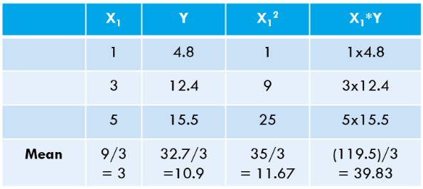
, let me take the simplest possible example. Consider the following 3 data points:
Everyone familiar with machine learning will immediately recognize that we are referring to X1 as the independent variable (also called “
Features
” or
“Attributes”),
and the Y is the dependent variable (also referred to as the
“Target”
or
“Outcome”).
Hence, the overall task of any machine is to find the relationship between X1 & Y. This relationship is actually
“learned”
by the machine from the
DATA.
Hence, we call the term Machine Learning. We, humans, learn from our experiences. Similarly, the same experience is fed into the machine as data.
Finding Best-Fit Line
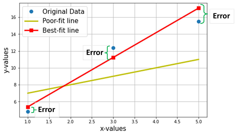
We want to find the best-fit line through the above 3 data points. The following plot shows these 3 data points in blue circles. Also shown is the red line (with squares), which we claim is the “best-fit line” through these 3 data points. I have also shown a “poor-fitting” line (the yellow line) for comparison.
The net objective is to find the Equation of the
Best-Fitting Straight Line
(through these 3 data points mentioned in the above table).
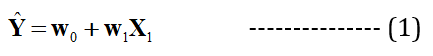
It is the equation of the best-fit line (red line in the above plot), where
w1
= slope of the line;
w0
= intercept of the line. In machine learning, this best fit is called the
Linear
Regression
(LR) model, and w0 and w1 are also called
model weights or model coefficients
.
Red-squares in the above plot represent the predicted values from the Linear Regression model (Y^). Of course, the predicted values are NOT the same as the actual values of Y (blue circles). The vertical difference represents the error in the prediction given by (see the image below) for any ith data point.
Now
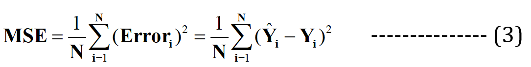
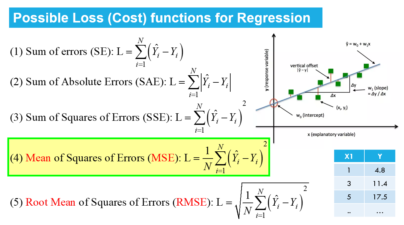
, I claim that this best-fit line will have the minimum error for prediction (among all possible infinite random “poor-fit” lines). This total error across all the data points is expressed as the
Mean Squared Error
(MSE) Function
, which will be the
minimum
for the best-fit line.
N = Total no. of data points in the dataset (in the current case, it is 3)
Minimizing or maximizing any quantity mathematically refers to an Optimization Problem, and the solution (the point where the minimum or maximum exists) indicates the optimal values of the variables.
Linear Regression
Linear Regression
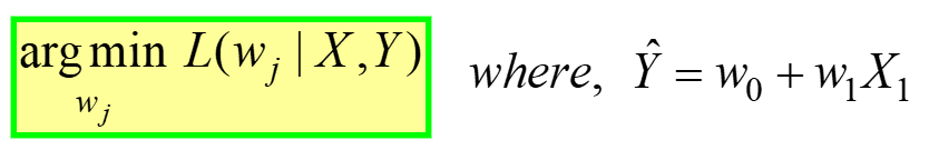
is an example of unconstrained optimization, given by:
———–
(4)
This is read as “Find the
optimal weights
(w
j
)
for which the
MSE
Loss function (given in eq. 3 above) has
min value,
for a
GIVEN X, Y data
” (refer to very first table at the start of the article).
L(w
j
)
represents the MSE Loss, a function of the model weights, not X or Y. Remember, X & Y is your DATA and is supposed to be CONSTANT! The subscript “j” represents the jth model coefficient/weight.
Upon substituting for Y^ = w
0
+ w
1
X
1
in the eq. 3 above, the final
MSE Loss Function (L)
looks as:
———–
(5)
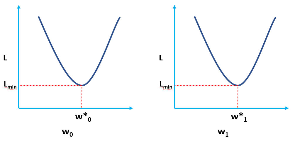
Clearly, L is a function of model weights (w
0
& w
1
), whose optimal values we have to find upon minimizing L. The optimal values are represented by (*) in the figure below.
OLS Solution in Scaler Form
The eq. 5 given above represents the OLS Loss function in the scaler form (where we can see the
summation of errors
for each data point. The OLS algorithm is an analytical solution to the optimization problem presented in the eq. 4. This analytical solution consists of the following steps:
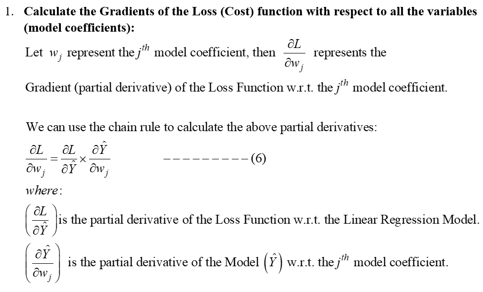
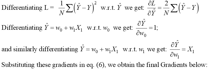
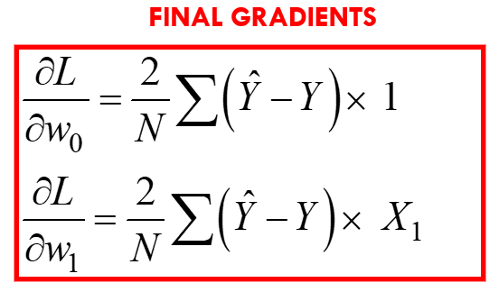
Step 1:
Step 2: Equate these gradients to zero and solve for the optimal values of the model coefficients w
j
.
This basically means that the slope of the tangent (the geometrical interpretation of the gradients) to the Loss function at the optimal values (the point where L is minimum) will be zero, as shown in the figures above.
From the above equations, we can shift the “2” from the LHS to the RHS; the RHS remains as 0 (as 0/2 is still 0).
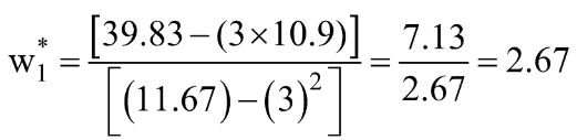
These expressions for w1* and w0* are the final OLS Analytical solution in the Scaler form.
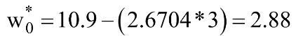
Step 3: Compute the above means and substitute in the expression for w1* & w0*.
Let’s calculate these values for our dataset:
Let us calculate the same using Python code:
[OUTPUT]: This is the Equation of the "Best-fit" Line:
2.675 x + 2.875
You can see our “hand-calculated” values match very closely the values of slope and intercept obtained using NumPy (the small difference is due to round-off errors in our hand-calculations). We can also verify that the same OLS is “running behind the scenes” of the LinearRegression class from the
scikit-learn
package, as demonstrated in the code below.
# import the LinearRegression class from scikit-learn package
from sklearn.linear_model import LinearRegression
LR = LinearRegression()
# create an instance of the LinearRegression class
# define your X and Y as NumPy Arrays (column vectors)
X = np.array([1,3,5]).reshape(-1,1)
Y = np.array([4.8,12.4,15.5]).reshape(-1,1)
LR.fit(X,Y)
# calculate the model coefficients
LR.intercept_
# the bias or the intercept term (w0*)
[Output]: array([2.875])
LR.coef_ # the slope term (w1*)
[Output]: array([[2.675]])
OLS in Action Using an Actual Example
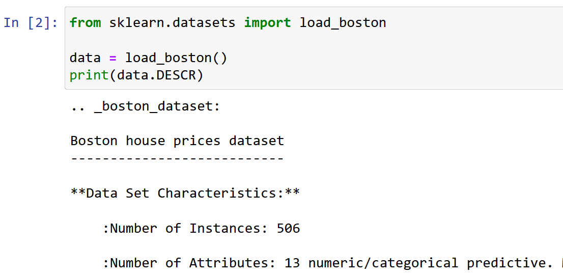
Here I am using the Boston House Pricing dataset, one of the most commonly encountered datasets while learning Data Science. The objective is to make a
Linear Regression Model
to Predict the median value of the House prices based on 13 features/attributes mentioned below.
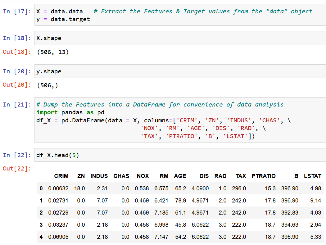
Import and explore the dataset.
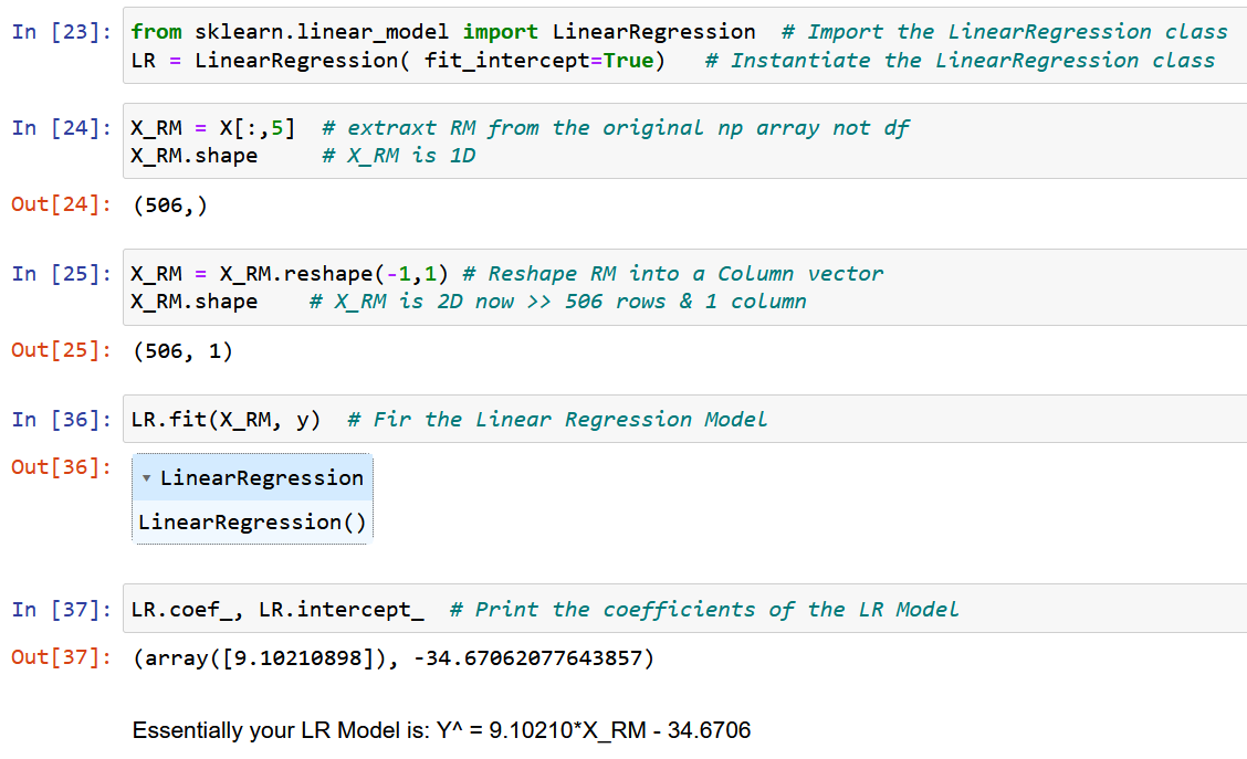
We’ll extract a single feature RM, the average room size in the given locality, and fit it with the target variable y (the median value of the house price).
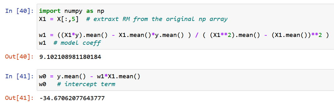
Now, let’s use pure NumPy and calculate the model coefficients using the expressions derived for the optimal values of the model coefficients w0 & w1 above (end of Step 2).
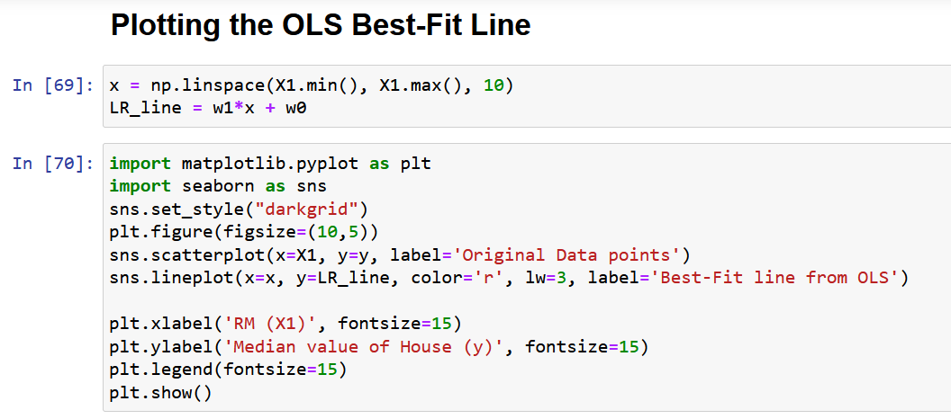
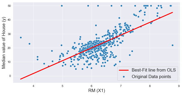
Let us finally plot the original data along with the best-fit line, as given below.
Problems with the Scaler Form of OLS Solution
Finally, let me discuss the main problem with the above approach, as described in section 4. As you can see from the abovementioned dataset, any real-life dataset will have multiple features. I took only one feature to demonstrate the OLS method in the above section because increasing the number of features also increases the number of gradients and the equations to solve simultaneously.
For 13 features (Boston dataset above), we’ll have 13 model coefficients and one intercept term, which brings the total number of variables to be optimized to 14. Hence, we’ll obtain 14 gradients (the partial derivative of the loss function concerning each of these 14 variables). Consequently, we need to solve 14 equations (after equating these 14 partial derivatives to zero, as described in step 2). You have already realized the complexity of the analytical solution with just 2 variables. Frankly, I have tried to give you the MOST elaborate explanation of OLS available on the internet, and yet it is not easy to assimilate the mathematics.
Hence, in simple words,
the above analytical solution is NOT SCALABLE!
The solution to this problem is the “Vectorized Form of the OLS Solution,” which I will discuss in detail in a follow-up article (Part 2 of this article), covering sections 7 & 8.
Conclusion
In conclusion, the OLS method is a powerful tool for estimating the parameters of a linear regression model. It is based on minimizing the sum of squared differences between the predicted and actual values.
I hope you enjoy the article and gain a clear understanding of the Ordinary Least Squares (OLS) regression, commonly referred to as the OLS model. This statistical technique estimates the relationships among variables. OLS linear regression minimizes the sum of squared differences, providing a robust method for predictive analysis in various fields.
Key Takeaway
Some of the key takeaways from the article are as follows:
The OLS solution represents itself in scalar form, making implementation and interpretation easy.
The article discussed optimization problems and the need for OLS in regression analysis and provided a mathematical formulation and an example of OLS in action.
The article also highlights some of the limitations of the scaler form of the OLS solution, such as scalability and the assumptions of linearity and constant variance. I hope you learned something new from this article. | ||||||||||||||||||
| Markdown | We use cookies essential for this site to function well. Please click to help us improve its usefulness with additional cookies. Learn about our use of cookies in our [Privacy Policy](https://www.analyticsvidhya.com/privacy-policy) & [Cookies Policy](https://www.analyticsvidhya.com/cookies-policy).
Show details
Accept all cookies
Use necessary cookies
[Master Generative AI with 10+ Real-world Projects in 2026! d h m s Download Projects](https://www.analyticsvidhya.com/pinnacleplus/pinnacleplus-projects?utm_source=blog_india&utm_medium=desktop_flashstrip&utm_campaign=15-Feb-2025||&utm_content=projects)
[](https://www.analyticsvidhya.com/blog/)
- [Free Courses](https://www.analyticsvidhya.com/courses/?ref=Navbar)
- [Accelerator Program](https://www.analyticsvidhya.com/ai-accelerator-program/?utm_source=blog&utm_medium=navbar) New
- [GenAI Pinnacle Plus](https://www.analyticsvidhya.com/pinnacleplus/?ref=blognavbar)
- [Agentic AI Pioneer](https://www.analyticsvidhya.com/agenticaipioneer/?ref=blognavbar)
- [DHS 2026](https://www.analyticsvidhya.com/datahacksummit?utm_source=blog&utm_medium=navbar)
- Login
- Switch Mode
- [Logout](https://www.analyticsvidhya.com/blog/2023/01/a-comprehensive-guide-to-ols-regression-part-1/)
[Interview Prep](https://www.analyticsvidhya.com/blog/category/interview-questions/?ref=category)
[Career](https://www.analyticsvidhya.com/blog/category/career/?ref=category)
[GenAI](https://www.analyticsvidhya.com/blog/category/generative-ai/?ref=category)
[Prompt Engg](https://www.analyticsvidhya.com/blog/category/prompt-engineering/?ref=category)
[ChatGPT](https://www.analyticsvidhya.com/blog/category/chatgpt/?ref=category)
[LLM](https://www.analyticsvidhya.com/blog/category/llms/?ref=category)
[Langchain](https://www.analyticsvidhya.com/blog/category/langchain/?ref=category)
[RAG](https://www.analyticsvidhya.com/blog/category/rag/?ref=category)
[AI Agents](https://www.analyticsvidhya.com/blog/category/ai-agent/?ref=category)
[Machine Learning](https://www.analyticsvidhya.com/blog/category/machine-learning/?ref=category)
[Deep Learning](https://www.analyticsvidhya.com/blog/category/deep-learning/?ref=category)
[GenAI Tools](https://www.analyticsvidhya.com/blog/category/ai-tools/?ref=category)
[LLMOps](https://www.analyticsvidhya.com/blog/category/llmops/?ref=category)
[Python](https://www.analyticsvidhya.com/blog/category/python/?ref=category)
[NLP](https://www.analyticsvidhya.com/blog/category/nlp/?ref=category)
[SQL](https://www.analyticsvidhya.com/blog/category/sql/?ref=category)
[AIML Projects](https://www.analyticsvidhya.com/blog/category/project/?ref=category)
#### Reading list
##### Intoduction to Python
[A Brief Introduction to Python](https://www.analyticsvidhya.com/blog/2016/01/complete-tutorial-learn-data-science-python-scratch-2/)[Installing Python in Windows, Linux, Mac](https://www.analyticsvidhya.com/blog/2019/08/everything-know-about-setting-up-python-windows-linux-and-mac/)[Jupyter Notebook](https://www.analyticsvidhya.com/blog/2021/05/5-must-have-jupyterlab-extension-for-data-science/)[Google Colab](https://www.analyticsvidhya.com/blog/2020/03/google-colab-machine-learning-deep-learning/)
##### Variables and data types
[Variables and Datatypes](https://www.analyticsvidhya.com/blog/2021/08/data-types-in-python-you-need-to-know-at-the-beginning-of-your-data-science-journey/)
##### OOPs Concepts
[OOPs Concepts](https://www.analyticsvidhya.com/blog/2020/09/object-oriented-programming/)
##### Conditional statement
[Conditional Statements](https://www.analyticsvidhya.com/blog/2021/09/loops-and-control-statements-an-in-depth-python-tutorial/)
##### Looping Constructs
[Looping Constructs](https://www.analyticsvidhya.com/blog/2016/01/python-tutorial-list-comprehension-examples/)[Iterators and Generators](https://www.analyticsvidhya.com/blog/2021/07/everything-you-should-know-about-iterables-and-iterators-in-python-as-a-data-scientist/)
##### Data Structures
[Data Structures](https://www.analyticsvidhya.com/blog/2021/07/everything-you-should-know-about-built-in-data-structures-in-python-a-beginners-guide/)[List and Tuples](https://www.analyticsvidhya.com/blog/2021/04/python-list-programs-for-absolute-beginners/)[Sets](https://www.analyticsvidhya.com/blog/2021/03/popular-python-data-structures-comparison-operations/)[Dictionary](https://www.analyticsvidhya.com/blog/2021/04/understand-the-concept-of-dictionary/)
##### String Manipulation
[Strings](https://www.analyticsvidhya.com/blog/2021/07/10-useful-python-string-functions-every-data-scientist-should-know-about/)
##### Functions
[Functions](https://www.analyticsvidhya.com/blog/2021/07/15-python-built-in-functions-which-you-should-know-while-learning-data-science/)[Lambda Functions](https://www.analyticsvidhya.com/blog/2020/03/what-are-lambda-functions-in-python/)[Recursion](https://www.analyticsvidhya.com/blog/2021/08/how-nested-functions-are-used-in-python/)
##### Modules, Packages and Standard Libraries
[Introduction to Modules in python](https://www.analyticsvidhya.com/blog/2021/07/working-with-modules-in-python-must-known-fundamentals-for-data-scientists/)
##### Python Libraries for Data Science
[Introduction to Python Libraries for Data Science](https://www.analyticsvidhya.com/blog/2020/11/top-13-python-libraries-every-data-science-aspirant-must-know-and-their-resources/)[Basics of Numpy](https://www.analyticsvidhya.com/blog/2020/04/the-ultimate-numpy-tutorial-for-data-science-beginners/)[Basics of Pandas](https://www.analyticsvidhya.com/blog/2022/08/the-ultimate-guide-to-pandas-for-data-science/)[Basics of Matplotlib](https://www.analyticsvidhya.com/blog/2020/10/headstart-to-plotting-graphs-using-matplotlib-library/)[Basics of Statsmodel](https://www.analyticsvidhya.com/blog/2021/05/learn-simple-linear-regression-slr/)
##### Reading Data Files in Python
[Reading Commonly Used File Formats](https://www.analyticsvidhya.com/blog/2017/03/read-commonly-used-formats-using-python/)[Reading CSV files](https://www.analyticsvidhya.com/blog/2021/08/python-tutorial-working-with-csv-file-for-data-science/)[Reading Big CSV files](https://www.analyticsvidhya.com/blog/2021/04/how-to-manipulate-a-20g-csv-file-efficiently/)[Reading Excel & Spreadsheet Files](https://www.analyticsvidhya.com/blog/2020/07/read-and-update-google-spreadsheets-with-python/)
##### Preprocessing, Subsetting and Modifying Pandas Dataframes
[Subsetting and Modifying Data](https://www.analyticsvidhya.com/blog/2022/02/exploratory-data-analysis-in-python/)[Loc vs ILoc](https://www.analyticsvidhya.com/blog/2020/02/loc-iloc-pandas/)
##### Sorting and Aggregating Data in Pandas
[Preprocessing, Sorting and Aggregating Data](https://www.analyticsvidhya.com/blog/2016/01/12-pandas-techniques-python-data-manipulation/)[Concatenating Dataframes](https://www.analyticsvidhya.com/blog/2020/02/joins-in-pandas-master-the-different-types-of-joins-in-python/)[Aggregating and Summarizing Dataframes](https://www.analyticsvidhya.com/blog/2020/03/groupby-pandas-aggregating-data-python/)[Data Munging](https://www.analyticsvidhya.com/blog/2021/03/pandas-functions-for-data-analysis-and-manipulation/)
##### Visualizing Patterns and Trends in Data
[Visualizing Patterns and Trends in Data](https://www.analyticsvidhya.com/blog/2021/02/data-visualization-bad-representation-of-data/)[Basics of Matplotlib](https://www.analyticsvidhya.com/blog/2021/10/introduction-to-matplotlib-using-python-for-beginners/)[Basics of Seaborn](https://www.analyticsvidhya.com/blog/2019/09/comprehensive-data-visualization-guide-seaborn-python/)[Data Visualization with Seaborn](https://www.analyticsvidhya.com/blog/2020/03/6-data-visualization-python-libraries/)[Exploring Data using Python](https://www.analyticsvidhya.com/blog/2015/06/infographic-cheat-sheet-data-exploration-python/)
##### Programming
[Tips and Technique to Optimize your Python Code](https://www.analyticsvidhya.com/blog/2020/07/5-striking-pandas-tips-and-tricks-for-analysts-and-data-scientists/)
1. [Home](https://www.analyticsvidhya.com/blog/)
2. [Machine Learning](https://www.analyticsvidhya.com/blog/category/machine-learning/)
3. A Comprehensive Guide to OLS Regression: Part-1
# A Comprehensive Guide to OLS Regression: Part-1
[P](https://www.analyticsvidhya.com/blog/author/prashant_sahu/)
[Prashant Sahu](https://www.analyticsvidhya.com/blog/author/prashant_sahu/) Last Updated : 28 Nov, 2024
10 min read
17
Ordinary Least squares is an optimization technique.OLS is the same technique that the scikit-learn LinearRegression class and the numpy.polyfit() function use behind the scenes. Before we proceed into the details of the OLS technique, it would be worthwhile going through the article I have written on the role of [**Optimization techniques in machine learning & deep learning**](https://www.analyticsvidhya.com/blog/2022/10/optimization-essentials-for-machine-learning/). In the same article, I have briefly explained the reason and context for the existence of the OLS technique (Section 6). This article continues the previous one, and I expect readers to be familiar with it.

Ordinary Least Squares (OLS) regression, commonly referred to as OLS, serves as a fundamental statistical method to model the relationship between a dependent variable and one or more independent variables. The OLS model minimizes the sum of the squared differences between observed and predicted values, ensuring the best fit for the data. OLS linear regression finds wide application in various fields, including economics and social sciences, providing valuable insights into data patterns and helping researchers make informed decisions based on their analyses. So here We have given What you learn in this article\!
**Learning Objectives:**
- Learn what OLS is and understand its mathematical equation
- Get an overview of OLS in scaler form and its drawbacks
- Understand OLS using a real-time example
## Table of contents
1. [What is the OLS Regression Model?](https://www.analyticsvidhya.com/blog/2023/01/a-comprehensive-guide-to-ols-regression-part-1/#h-what-is-the-ols-regression-model)
2. [What are Optimization Problems?](https://www.analyticsvidhya.com/blog/2023/01/a-comprehensive-guide-to-ols-regression-part-1/#h-what-are-optimization-problems)
3. [Why Do We Need OLS?](https://www.analyticsvidhya.com/blog/2023/01/a-comprehensive-guide-to-ols-regression-part-1/#h-why-do-we-need-ols)
4. [OLS Solution in Scaler Form](https://www.analyticsvidhya.com/blog/2023/01/a-comprehensive-guide-to-ols-regression-part-1/#h-ols-solution-in-scaler-form)
5. [OLS in Action Using an Actual Example](https://www.analyticsvidhya.com/blog/2023/01/a-comprehensive-guide-to-ols-regression-part-1/#h-ols-in-action-using-an-actual-example)
6. [Problems with the Scaler Form of OLS Solution](https://www.analyticsvidhya.com/blog/2023/01/a-comprehensive-guide-to-ols-regression-part-1/#h-problems-with-the-scaler-form-of-ols-solution)
7. [Conclusion](https://www.analyticsvidhya.com/blog/2023/01/a-comprehensive-guide-to-ols-regression-part-1/#h-conclusion)
- [Key Takeaway](https://www.analyticsvidhya.com/blog/2023/01/a-comprehensive-guide-to-ols-regression-part-1/#h-key-takeaway)
[Free Certification Courses Machine Learning Certification for Beginners Understand Python basics • Data processing with pandas • Stats-driven EDA Get Certified Now](https://www.analyticsvidhya.com/courses/Machine-Learning-Certification-Course-for-Beginners/?utm_source=blog&utm_medium=free_course_banner&utm_term=free_course_auto_enrollment)
## What is the OLS Regression Model?
OLS regression is a statistical method utilized for parameter estimation in linear regression models. Ordinary least squares (OLS) aim to find the optimal line that minimizes the total squared differences between the actual and estimated values of the dependent variable.
**The key components of OLS Linear Regression are:**.
- It demonstrates the linear relationship between a response variable (y) and one or more predictor variables (x).
- The linear equation is y = β0 + β1×1 + β2×2 + … + βpxp + ε, where β0 is the intercept, β1 to βp are the coefficients for x1 to xp, and ε is the error term.
- OLS chooses β0, β1, …, βp to minimize the sum of squared differences between the observed y values and the predicted y values from the regression line.
- If the OLS estimators meet certain conditions like linearity, lack of multicollinearity, homoscedasticity, absence of autocorrelation, and normality of errors, they will be unbiased, consistent, and have the lowest variance among linear unbiased estimators.
## What are Optimization Problems?
Optimization problems are mathematical problems that involve finding the best solution from a set of possible solutions. These problems typically present themselves as maximization or minimization problems, aiming to maximize or minimize a certain objective function. The objective function serves as a mathematical expression that describes the quantity to optimize, while a set of constraints defines the possible solutions.
Optimization problems arise in various fields, including engineering, finance, economics, and operations research. They are used to model and solve problems such as resource allocation, scheduling, and portfolio optimization. Optimization is a crucial component of many machine learning algorithms. In machine learning, optimization helps find the best set of parameters for a model that minimizes the difference between the model’s predictions and the true values. Researchers actively explore optimization as a key area in machine learning, developing new algorithms to improve the speed and accuracy of training models.
#### Examples
Some examples of where optimization is used in machine learning include:
- **In supervised learning**, optimization is used to find the parameters of a model that minimize the difference between the model’s predictions and the true values for a given training dataset. For example, linear regression and logistic regression use optimization to find the best values of the model’s coefficients. In addition, some models, like decision trees, random forests, and gradient boosting models, build by iteratively adding new models to the ensemble and optimizing the parameters of the new models to minimize the error on the training data.
- **In unsupervised learning**, optimization helps to find the best configuration of clusters or mapping of the data that best represents the underlying structure in the data. In **clustering**, optimization is used to find the best cluster configuration in the data. For example, the K-Means algorithm uses an optimization technique called Lloyd’s algorithm, which iteratively reassigns data points to the nearest cluster centroid and updates the cluster centroids based on the newly assigned points. Similarly, other clustering algorithms, such as hierarchical, density-based, and Gaussian mixture models, also use optimization techniques to find the best clustering solution. In dimensionality reduction, optimization finds the best data mapping from a high- to a lower-dimensional space. For example, Principal Component Analysis (PCA) uses Singular Value Decomposition (SVD), an optimization technique, to find the best linear combination of the original variables that explains the most variance in the data. Other dimensionality reduction techniques like Linear Discriminant Analysis (LDA) and t-distributed Stochastic Neighbor Embedding (t-SNE) also use optimization techniques to find the best data representation in a lower-dimensional space.
- In **deep learning**, optimization helps find the best set of parameters for neural networks, typically using gradient-based optimization algorithms such as stochastic gradient descent (SGD) or Adam/Adagrad/RMSProp.
## Why Do We Need OLS?
The [**ordinary least squares**](https://www.xlstat.com/en/solutions/features/ordinary-least-squares-regression-ols) (OLS) algorithm is a method for estimating the parameters of a linear regression model. The OLS algorithm aims to find the values of the linear regression model’s parameters (i.e., the coefficients) that minimize the sum of the squared residuals. The residuals are the differences between the observed values of the dependent variable and the predicted values of the dependent variable given the independent variables. It is important to note that the OLS algorithm assumes the errors follow a normal distribution with zero mean and constant variance, and it assumes no multicollinearity (high correlation) among the independent variables. Use other methods, such as Generalized Least Squares or Weighted Least Squares, when these assumptions are unmet.
## Understanding the Mathematics behind the OLS Algorithm
To explain the OLS [**algorithm**](https://github.com/jorgesleonel/linear-regression), let me take the simplest possible example. Consider the following 3 data points:
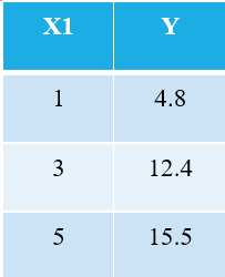

Everyone familiar with machine learning will immediately recognize that we are referring to X1 as the independent variable (also called “**Features**” or **“Attributes”),** and the Y is the dependent variable (also referred to as the **“Target”** or **“Outcome”).** Hence, the overall task of any machine is to find the relationship between X1 & Y. This relationship is actually **“learned”** by the machine from the **DATA.** Hence, we call the term Machine Learning. We, humans, learn from our experiences. Similarly, the same experience is fed into the machine as data.
#### Finding Best-Fit Line
We want to find the best-fit line through the above 3 data points. The following plot shows these 3 data points in blue circles. Also shown is the red line (with squares), which we claim is the “best-fit line” through these 3 data points. I have also shown a “poor-fitting” line (the yellow line) for comparison.
The net objective is to find the Equation of the **Best-Fitting Straight Line** (through these 3 data points mentioned in the above table).
It is the equation of the best-fit line (red line in the above plot), where **w1** = slope of the line; **w0** = intercept of the line. In machine learning, this best fit is called the **Linear** **Regression** (LR) model, and w0 and w1 are also called **model weights or model coefficients**.
Red-squares in the above plot represent the predicted values from the Linear Regression model (Y^). Of course, the predicted values are NOT the same as the actual values of Y (blue circles). The vertical difference represents the error in the prediction given by (see the image below) for any ith data point.
Now, I claim that this best-fit line will have the minimum error for prediction (among all possible infinite random “poor-fit” lines). This total error across all the data points is expressed as the **Mean Squared Error** **(MSE) Function**, which will be the **minimum** for the best-fit line.
N = Total no. of data points in the dataset (in the current case, it is 3)
Minimizing or maximizing any quantity mathematically refers to an Optimization Problem, and the solution (the point where the minimum or maximum exists) indicates the optimal values of the variables.
#### Linear Regression
**[Linear Regression](https://www.analyticsvidhya.com/blog/2022/03/multiple-linear-regression-using-python/)** is an example of unconstrained optimization, given by:
———– **(4)**
This is read as “Find the **optimal weights** **(wj)** for which the **MSE** Loss function (given in eq. 3 above) has **min value,** for a **GIVEN X, Y data**” (refer to very first table at the start of the article). **L(wj)** represents the MSE Loss, a function of the model weights, not X or Y. Remember, X & Y is your DATA and is supposed to be CONSTANT! The subscript “j” represents the jth model coefficient/weight.
Upon substituting for Y^ = w0 + w1X1 in the eq. 3 above, the final **MSE Loss Function (L)** looks as:

———– **(5)**
Clearly, L is a function of model weights (w0 & w1), whose optimal values we have to find upon minimizing L. The optimal values are represented by (\*) in the figure below.
## OLS Solution in Scaler Form
The eq. 5 given above represents the OLS Loss function in the scaler form (where we can see the *summation of errors* for each data point. The OLS algorithm is an analytical solution to the optimization problem presented in the eq. 4. This analytical solution consists of the following steps:
**Step 1:**
**Step 2: Equate these gradients to zero and solve for the optimal values of the model coefficients wj.**
This basically means that the slope of the tangent (the geometrical interpretation of the gradients) to the Loss function at the optimal values (the point where L is minimum) will be zero, as shown in the figures above.

From the above equations, we can shift the “2” from the LHS to the RHS; the RHS remains as 0 (as 0/2 is still 0).


**These expressions for w1\* and w0\* are the final OLS Analytical solution in the Scaler form.**
**Step 3: Compute the above means and substitute in the expression for w1\* & w0\*.**
Let’s calculate these values for our dataset:
*Let us calculate the same using Python code:*
```
scaler form of OLS solution
[OUTPUT]: This is the Equation of the "Best-fit" Line:
2.675 x + 2.875
```
You can see our “hand-calculated” values match very closely the values of slope and intercept obtained using NumPy (the small difference is due to round-off errors in our hand-calculations). We can also verify that the same OLS is “running behind the scenes” of the LinearRegression class from the [**scikit-learn**](https://www.analyticsvidhya.com/blog/2021/08/complete-guide-on-how-to-learn-scikit-learn-for-data-science/) package, as demonstrated in the code below.
```
Copy Code
```
```
[Output]: array([2.875])
```
```
LR.coef_ # the slope term (w1*)
[Output]: array([[2.675]])
```
## OLS in Action Using an Actual Example
Here I am using the Boston House Pricing dataset, one of the most commonly encountered datasets while learning Data Science. The objective is to make a [**Linear Regression Model**](https://www.analyticsvidhya.com/blog/2022/06/linear-regression-using-mlib/) to Predict the median value of the House prices based on 13 features/attributes mentioned below.
Import and explore the dataset.
We’ll extract a single feature RM, the average room size in the given locality, and fit it with the target variable y (the median value of the house price).
Now, let’s use pure NumPy and calculate the model coefficients using the expressions derived for the optimal values of the model coefficients w0 & w1 above (end of Step 2).
Let us finally plot the original data along with the best-fit line, as given below.
## Problems with the Scaler Form of OLS Solution
Finally, let me discuss the main problem with the above approach, as described in section 4. As you can see from the abovementioned dataset, any real-life dataset will have multiple features. I took only one feature to demonstrate the OLS method in the above section because increasing the number of features also increases the number of gradients and the equations to solve simultaneously.
For 13 features (Boston dataset above), we’ll have 13 model coefficients and one intercept term, which brings the total number of variables to be optimized to 14. Hence, we’ll obtain 14 gradients (the partial derivative of the loss function concerning each of these 14 variables). Consequently, we need to solve 14 equations (after equating these 14 partial derivatives to zero, as described in step 2). You have already realized the complexity of the analytical solution with just 2 variables. Frankly, I have tried to give you the MOST elaborate explanation of OLS available on the internet, and yet it is not easy to assimilate the mathematics.
Hence, in simple words, **the above analytical solution is NOT SCALABLE\!**
The solution to this problem is the “Vectorized Form of the OLS Solution,” which I will discuss in detail in a follow-up article (Part 2 of this article), covering sections 7 & 8.
## Conclusion
In conclusion, the OLS method is a powerful tool for estimating the parameters of a linear regression model. It is based on minimizing the sum of squared differences between the predicted and actual values.
I hope you enjoy the article and gain a clear understanding of the Ordinary Least Squares (OLS) regression, commonly referred to as the OLS model. This statistical technique estimates the relationships among variables. OLS linear regression minimizes the sum of squared differences, providing a robust method for predictive analysis in various fields.
### Key Takeaway
Some of the key takeaways from the article are as follows:
- The OLS solution represents itself in scalar form, making implementation and interpretation easy.
- The article discussed optimization problems and the need for OLS in regression analysis and provided a mathematical formulation and an example of OLS in action.
- The article also highlights some of the limitations of the scaler form of the OLS solution, such as scalability and the assumptions of linearity and constant variance. I hope you learned something new from this article.
[P](https://www.analyticsvidhya.com/blog/author/prashant_sahu/)
[Prashant Sahu](https://www.analyticsvidhya.com/blog/author/prashant_sahu/)
[Intermediate](https://www.analyticsvidhya.com/blog/category/intermediate/)[Linear Regression](https://www.analyticsvidhya.com/blog/category/machine-learning/linear-regression/)[Machine Learning](https://www.analyticsvidhya.com/blog/category/machine-learning/)[Maths](https://www.analyticsvidhya.com/blog/category/maths/)[Python](https://www.analyticsvidhya.com/blog/category/python/)[Python](https://www.analyticsvidhya.com/blog/category/python-2/)[Technique](https://www.analyticsvidhya.com/blog/category/technique/)
#### Login to continue reading and enjoy expert-curated content.
Keep Reading for Free
## Free Courses
[ 4.5 Model Deployment using FastAPI; Prepare, Train, and Test FastAPI Application Deploy a fastapi machine learning model with XGBoost and Docker APIs.](https://www.analyticsvidhya.com/courses/model-deployment-using-fastapi/?utm_source=blog&utm_medium=free_course_recommendation)
[ 5 Build Data Pipelines with Apache Airflow Learn ETL pipeline building and workflow orchestration with Airflow.](https://www.analyticsvidhya.com/courses/build-data-pipelines-with-apache-airflow/?utm_source=blog&utm_medium=free_course_recommendation)
[ 4.6 Evaluation Metrics for Machine Learning Models This course covers evaluation metrics to improve ML model performance.](https://www.analyticsvidhya.com/courses/evaluation-metrics-for-machine-learning-models/?utm_source=blog&utm_medium=free_course_recommendation)
[ 4.8 The A to Z of Unsupervised Machine Learning Learn Unsupervised ML & DBSCAN with real-world applications.](https://www.analyticsvidhya.com/courses/free-unsupervised-ml-guide/?utm_source=blog&utm_medium=free_course_recommendation)
[ 4.8 K-Nearest Neighbors (KNN) Algorithm in Python and R Master KNN algorithm with hands-on Python & R tutorials.](https://www.analyticsvidhya.com/courses/K-Nearest-Neighbors-KNN-Algorithm/?utm_source=blog&utm_medium=free_course_recommendation)
#### Recommended Articles
- [GPT-4 vs. Llama 3.1 – Which Model is Better?](https://www.analyticsvidhya.com/blog/2024/08/gpt-4-vs-llama-3-1/)
- [Llama-3.1-Storm-8B: The 8B LLM Powerhouse Surpa...](https://www.analyticsvidhya.com/blog/2024/08/llama-3-1-storm-8b/)
- [A Comprehensive Guide to Building Agentic RAG S...](https://www.analyticsvidhya.com/blog/2024/07/building-agentic-rag-systems-with-langgraph/)
- [Top 10 Machine Learning Algorithms in 2026](https://www.analyticsvidhya.com/blog/2017/09/common-machine-learning-algorithms/)
- [45 Questions to Test a Data Scientist on Basics...](https://www.analyticsvidhya.com/blog/2017/01/must-know-questions-deep-learning/)
- [90+ Python Interview Questions and Answers (202...](https://www.analyticsvidhya.com/blog/2022/07/python-coding-interview-questions-for-freshers/)
- [8 Easy Ways to Access ChatGPT for Free](https://www.analyticsvidhya.com/blog/2023/12/chatgpt-4-for-free/)
- [Prompt Engineering: Definition, Examples, Tips ...](https://www.analyticsvidhya.com/blog/2023/06/what-is-prompt-engineering/)
- [What is LangChain?](https://www.analyticsvidhya.com/blog/2024/06/langchain-guide/)
- [What is Retrieval-Augmented Generation (RAG)?](https://www.analyticsvidhya.com/blog/2023/09/retrieval-augmented-generation-rag-in-ai/)
### Responses From Readers
[Cancel reply](https://www.analyticsvidhya.com/blog/2023/01/a-comprehensive-guide-to-ols-regression-part-1/#respond)

RIZWAN ALI
very informative. looking for part 2. also real-world code / example and metric discussion in business cases
123
[Cancel reply](https://www.analyticsvidhya.com/blog/2023/01/a-comprehensive-guide-to-ols-regression-part-1/#respond)
[Become an Author Share insights, grow your voice, and inspire the data community.](https://www.analyticsvidhya.com/become-an-author)
[Reach a Global Audience Share Your Expertise with the World Build Your Brand & Audience Join a Thriving AI Community Level Up Your AI Game Expand Your Influence in Genrative AI](https://www.analyticsvidhya.com/become-an-author)
[](https://www.analyticsvidhya.com/become-an-author)
## Flagship Programs
[GenAI Pinnacle Program](https://www.analyticsvidhya.com/genaipinnacle/?ref=footer)\| [GenAI Pinnacle Plus Program](https://www.analyticsvidhya.com/pinnacleplus/?ref=blogflashstripfooter)\| [AI/ML BlackBelt Program](https://www.analyticsvidhya.com/bbplus?ref=footer)\| [Agentic AI Pioneer Program](https://www.analyticsvidhya.com/agenticaipioneer?ref=footer)
## Free Courses
[Generative AI](https://www.analyticsvidhya.com/courses/genai-a-way-of-life/?ref=footer)\| [DeepSeek](https://www.analyticsvidhya.com/courses/getting-started-with-deepseek/?ref=footer)\| [OpenAI Agent SDK](https://www.analyticsvidhya.com/courses/demystifying-openai-agents-sdk/?ref=footer)\| [LLM Applications using Prompt Engineering](https://www.analyticsvidhya.com/courses/building-llm-applications-using-prompt-engineering-free/?ref=footer)\| [DeepSeek from Scratch](https://www.analyticsvidhya.com/courses/deepseek-from-scratch/?ref=footer)\| [Stability.AI](https://www.analyticsvidhya.com/courses/exploring-stability-ai/?ref=footer)\| [SSM & MAMBA](https://www.analyticsvidhya.com/courses/building-smarter-llms-with-mamba-and-state-space-model/?ref=footer)\| [RAG Systems using LlamaIndex](https://www.analyticsvidhya.com/courses/building-first-rag-systems-using-llamaindex/?ref=footer)\| [Building LLMs for Code](https://www.analyticsvidhya.com/courses/building-large-language-models-for-code/?ref=footer)\| [Python](https://www.analyticsvidhya.com/courses/introduction-to-data-science/?ref=footer)\| [Microsoft Excel](https://www.analyticsvidhya.com/courses/microsoft-excel-formulas-functions/?ref=footer)\| [Machine Learning](https://www.analyticsvidhya.com/courses/Machine-Learning-Certification-Course-for-Beginners/?ref=footer)\| [Deep Learning](https://www.analyticsvidhya.com/courses/getting-started-with-deep-learning/?ref=footer)\| [Mastering Multimodal RAG](https://www.analyticsvidhya.com/courses/mastering-multimodal-rag-and-embeddings-with-amazon-nova-and-bedrock/?ref=footer)\| [Introduction to Transformer Model](https://www.analyticsvidhya.com/courses/introduction-to-transformers-and-attention-mechanisms/?ref=footer)\| [Bagging & Boosting](https://www.analyticsvidhya.com/courses/bagging-boosting-ML-Algorithms/?ref=footer)\| [Loan Prediction](https://www.analyticsvidhya.com/courses/loan-prediction-practice-problem-using-python/?ref=footer)\| [Time Series Forecasting](https://www.analyticsvidhya.com/courses/creating-time-series-forecast-using-python/?ref=footer)\| [Tableau](https://www.analyticsvidhya.com/courses/tableau-for-beginners/?ref=footer)\| [Business Analytics](https://www.analyticsvidhya.com/courses/introduction-to-analytics/?ref=footer)\| [Vibe Coding in Windsurf](https://www.analyticsvidhya.com/courses/guide-to-vibe-coding-in-windsurf/?ref=footer)\| [Model Deployment using FastAPI](https://www.analyticsvidhya.com/courses/model-deployment-using-fastapi/?ref=footer)\| [Building Data Analyst AI Agent](https://www.analyticsvidhya.com/courses/building-data-analyst-AI-agent/?ref=footer)\| [Getting started with OpenAI o3-mini](https://www.analyticsvidhya.com/courses/getting-started-with-openai-o3-mini/?ref=footer)\| [Introduction to Transformers and Attention Mechanisms](https://www.analyticsvidhya.com/courses/introduction-to-transformers-and-attention-mechanisms/?ref=footer)
## Popular Categories
[AI Agents](https://www.analyticsvidhya.com/blog/category/ai-agent/?ref=footer)\| [Generative AI](https://www.analyticsvidhya.com/blog/category/generative-ai/?ref=footer)\| [Prompt Engineering](https://www.analyticsvidhya.com/blog/category/prompt-engineering/?ref=footer)\| [Generative AI Application](https://www.analyticsvidhya.com/blog/category/generative-ai-application/?ref=footer)\| [News](https://news.google.com/publications/CAAqBwgKMJiWzAswyLHjAw?hl=en-IN&gl=IN&ceid=IN%3Aen)\| [Technical Guides](https://www.analyticsvidhya.com/blog/category/guide/?ref=footer)\| [AI Tools](https://www.analyticsvidhya.com/blog/category/ai-tools/?ref=footer)\| [Interview Preparation](https://www.analyticsvidhya.com/blog/category/interview-questions/?ref=footer)\| [Research Papers](https://www.analyticsvidhya.com/blog/category/research-paper/?ref=footer)\| [Success Stories](https://www.analyticsvidhya.com/blog/category/success-story/?ref=footer)\| [Quiz](https://www.analyticsvidhya.com/blog/category/quiz/?ref=footer)\| [Use Cases](https://www.analyticsvidhya.com/blog/category/use-cases/?ref=footer)\| [Listicles](https://www.analyticsvidhya.com/blog/category/listicle/?ref=footer)
## Generative AI Tools and Techniques
[GANs](https://www.analyticsvidhya.com/blog/2021/10/an-end-to-end-introduction-to-generative-adversarial-networksgans/?ref=footer)\| [VAEs](https://www.analyticsvidhya.com/blog/2023/07/an-overview-of-variational-autoencoders/?ref=footer)\| [Transformers](https://www.analyticsvidhya.com/blog/2019/06/understanding-transformers-nlp-state-of-the-art-models?ref=footer)\| [StyleGAN](https://www.analyticsvidhya.com/blog/2021/05/stylegan-explained-in-less-than-five-minutes/?ref=footer)\| [Pix2Pix](https://www.analyticsvidhya.com/blog/2023/10/pix2pix-unleashed-transforming-images-with-creative-superpower?ref=footer)\| [Autoencoders](https://www.analyticsvidhya.com/blog/2021/06/autoencoders-a-gentle-introduction?ref=footer)\| [GPT](https://www.analyticsvidhya.com/blog/2022/10/generative-pre-training-gpt-for-natural-language-understanding/?ref=footer)\| [BERT](https://www.analyticsvidhya.com/blog/2022/11/comprehensive-guide-to-bert/?ref=footer)\| [Word2Vec](https://www.analyticsvidhya.com/blog/2021/07/word2vec-for-word-embeddings-a-beginners-guide/?ref=footer)\| [LSTM](https://www.analyticsvidhya.com/blog/2021/03/introduction-to-long-short-term-memory-lstm?ref=footer)\| [Attention Mechanisms](https://www.analyticsvidhya.com/blog/2019/11/comprehensive-guide-attention-mechanism-deep-learning/?ref=footer)\| [Diffusion Models](https://www.analyticsvidhya.com/blog/2024/09/what-are-diffusion-models/?ref=footer)\| [LLMs](https://www.analyticsvidhya.com/blog/2023/03/an-introduction-to-large-language-models-llms/?ref=footer)\| [SLMs](https://www.analyticsvidhya.com/blog/2024/05/what-are-small-language-models-slms/?ref=footer)\| [Encoder Decoder Models](https://www.analyticsvidhya.com/blog/2023/10/advanced-encoders-and-decoders-in-generative-ai/?ref=footer)\| [Prompt Engineering](https://www.analyticsvidhya.com/blog/2023/06/what-is-prompt-engineering/?ref=footer)\| [LangChain](https://www.analyticsvidhya.com/blog/2024/06/langchain-guide/?ref=footer)\| [LlamaIndex](https://www.analyticsvidhya.com/blog/2023/10/rag-pipeline-with-the-llama-index/?ref=footer)\| [RAG](https://www.analyticsvidhya.com/blog/2023/09/retrieval-augmented-generation-rag-in-ai/?ref=footer)\| [Fine-tuning](https://www.analyticsvidhya.com/blog/2023/08/fine-tuning-large-language-models/?ref=footer)\| [LangChain AI Agent](https://www.analyticsvidhya.com/blog/2024/07/langchains-agent-framework/?ref=footer)\| [Multimodal Models](https://www.analyticsvidhya.com/blog/2023/12/what-are-multimodal-models/?ref=footer)\| [RNNs](https://www.analyticsvidhya.com/blog/2022/03/a-brief-overview-of-recurrent-neural-networks-rnn/?ref=footer)\| [DCGAN](https://www.analyticsvidhya.com/blog/2021/07/deep-convolutional-generative-adversarial-network-dcgan-for-beginners/?ref=footer)\| [ProGAN](https://www.analyticsvidhya.com/blog/2021/05/progressive-growing-gan-progan/?ref=footer)\| [Text-to-Image Models](https://www.analyticsvidhya.com/blog/2024/02/llm-driven-text-to-image-with-diffusiongpt/?ref=footer)\| [DDPM](https://www.analyticsvidhya.com/blog/2024/08/different-components-of-diffusion-models/?ref=footer)\| [Document Question Answering](https://www.analyticsvidhya.com/blog/2024/04/a-hands-on-guide-to-creating-a-pdf-based-qa-assistant-with-llama-and-llamaindex/?ref=footer)\| [Imagen](https://www.analyticsvidhya.com/blog/2024/09/google-imagen-3/?ref=footer)\| [T5 (Text-to-Text Transfer Transformer)](https://www.analyticsvidhya.com/blog/2024/05/text-summarization-using-googles-t5-base/?ref=footer)\| [Seq2seq Models](https://www.analyticsvidhya.com/blog/2020/08/a-simple-introduction-to-sequence-to-sequence-models/?ref=footer)\| [WaveNet](https://www.analyticsvidhya.com/blog/2020/01/how-to-perform-automatic-music-generation/?ref=footer)\| [Attention Is All You Need (Transformer Architecture)](https://www.analyticsvidhya.com/blog/2019/11/comprehensive-guide-attention-mechanism-deep-learning/?ref=footer) \| [WindSurf](https://www.analyticsvidhya.com/blog/2024/11/windsurf-editor/?ref=footer)\| [Cursor](https://www.analyticsvidhya.com/blog/2025/03/vibe-coding-with-cursor-ai/?ref=footer)
## Popular GenAI Models
[Llama 4](https://www.analyticsvidhya.com/blog/2025/04/meta-llama-4/?ref=footer)\| [Llama 3.1](https://www.analyticsvidhya.com/blog/2024/07/meta-llama-3-1/?ref=footer)\| [GPT 4.5](https://www.analyticsvidhya.com/blog/2025/02/openai-gpt-4-5/?ref=footer)\| [GPT 4.1](https://www.analyticsvidhya.com/blog/2025/04/open-ai-gpt-4-1/?ref=footer)\| [GPT 4o](https://www.analyticsvidhya.com/blog/2025/03/updated-gpt-4o/?ref=footer)\| [o3-mini](https://www.analyticsvidhya.com/blog/2025/02/openai-o3-mini/?ref=footer)\| [Sora](https://www.analyticsvidhya.com/blog/2024/12/openai-sora/?ref=footer)\| [DeepSeek R1](https://www.analyticsvidhya.com/blog/2025/01/deepseek-r1/?ref=footer)\| [DeepSeek V3](https://www.analyticsvidhya.com/blog/2025/01/ai-application-with-deepseek-v3/?ref=footer)\| [Janus Pro](https://www.analyticsvidhya.com/blog/2025/01/deepseek-janus-pro-7b/?ref=footer)\| [Veo 2](https://www.analyticsvidhya.com/blog/2024/12/googles-veo-2/?ref=footer)\| [Gemini 2.5 Pro](https://www.analyticsvidhya.com/blog/2025/03/gemini-2-5-pro-experimental/?ref=footer)\| [Gemini 2.0](https://www.analyticsvidhya.com/blog/2025/02/gemini-2-0-everything-you-need-to-know-about-googles-latest-llms/?ref=footer)\| [Gemma 3](https://www.analyticsvidhya.com/blog/2025/03/gemma-3/?ref=footer)\| [Claude Sonnet 3.7](https://www.analyticsvidhya.com/blog/2025/02/claude-sonnet-3-7/?ref=footer)\| [Claude 3.5 Sonnet](https://www.analyticsvidhya.com/blog/2024/06/claude-3-5-sonnet/?ref=footer)\| [Phi 4](https://www.analyticsvidhya.com/blog/2025/02/microsoft-phi-4-multimodal/?ref=footer)\| [Phi 3.5](https://www.analyticsvidhya.com/blog/2024/09/phi-3-5-slms/?ref=footer)\| [Mistral Small 3.1](https://www.analyticsvidhya.com/blog/2025/03/mistral-small-3-1/?ref=footer)\| [Mistral NeMo](https://www.analyticsvidhya.com/blog/2024/08/mistral-nemo/?ref=footer)\| [Mistral-7b](https://www.analyticsvidhya.com/blog/2024/01/making-the-most-of-mistral-7b-with-finetuning/?ref=footer)\| [Bedrock](https://www.analyticsvidhya.com/blog/2024/02/building-end-to-end-generative-ai-models-with-aws-bedrock/?ref=footer)\| [Vertex AI](https://www.analyticsvidhya.com/blog/2024/02/build-deploy-and-manage-ml-models-with-google-vertex-ai/?ref=footer)\| [Qwen QwQ 32B](https://www.analyticsvidhya.com/blog/2025/03/qwens-qwq-32b/?ref=footer)\| [Qwen 2](https://www.analyticsvidhya.com/blog/2024/06/qwen2/?ref=footer)\| [Qwen 2.5 VL](https://www.analyticsvidhya.com/blog/2025/01/qwen2-5-vl-vision-model/?ref=footer)\| [Qwen Chat](https://www.analyticsvidhya.com/blog/2025/03/qwen-chat/?ref=footer)\| [Grok 3](https://www.analyticsvidhya.com/blog/2025/02/grok-3/?ref=footer)
## AI Development Frameworks
[n8n](https://www.analyticsvidhya.com/blog/2025/03/content-creator-agent-with-n8n/?ref=footer)\| [LangChain](https://www.analyticsvidhya.com/blog/2024/06/langchain-guide/?ref=footer)\| [Agent SDK](https://www.analyticsvidhya.com/blog/2025/03/open-ai-responses-api/?ref=footer)\| [A2A by Google](https://www.analyticsvidhya.com/blog/2025/04/agent-to-agent-protocol/?ref=footer)\| [SmolAgents](https://www.analyticsvidhya.com/blog/2025/01/smolagents/?ref=footer)\| [LangGraph](https://www.analyticsvidhya.com/blog/2024/07/langgraph-revolutionizing-ai-agent/?ref=footer)\| [CrewAI](https://www.analyticsvidhya.com/blog/2024/01/building-collaborative-ai-agents-with-crewai/?ref=footer)\| [Agno](https://www.analyticsvidhya.com/blog/2025/03/agno-framework/?ref=footer)\| [LangFlow](https://www.analyticsvidhya.com/blog/2023/06/langflow-ui-for-langchain-to-develop-applications-with-llms/?ref=footer)\| [AutoGen](https://www.analyticsvidhya.com/blog/2023/11/launching-into-autogen-exploring-the-basics-of-a-multi-agent-framework/?ref=footer)\| [LlamaIndex](https://www.analyticsvidhya.com/blog/2024/08/implementing-ai-agents-using-llamaindex/?ref=footer)\| [Swarm](https://www.analyticsvidhya.com/blog/2024/12/managing-multi-agent-systems-with-openai-swarm/?ref=footer)\| [AutoGPT](https://www.analyticsvidhya.com/blog/2023/05/learn-everything-about-autogpt/?ref=footer)
## Data Science Tools and Techniques
[Python](https://www.analyticsvidhya.com/blog/2016/01/complete-tutorial-learn-data-science-python-scratch-2/?ref=footer)\| [R](https://www.analyticsvidhya.com/blog/2016/02/complete-tutorial-learn-data-science-scratch/?ref=footer)\| [SQL](https://www.analyticsvidhya.com/blog/2022/01/learning-sql-from-basics-to-advance/?ref=footer)\| [Jupyter Notebooks](https://www.analyticsvidhya.com/blog/2018/05/starters-guide-jupyter-notebook/?ref=footer)\| [TensorFlow](https://www.analyticsvidhya.com/blog/2021/11/tensorflow-for-beginners-with-examples-and-python-implementation/?ref=footer)\| [Scikit-learn](https://www.analyticsvidhya.com/blog/2021/08/complete-guide-on-how-to-learn-scikit-learn-for-data-science/?ref=footer)\| [PyTorch](https://www.analyticsvidhya.com/blog/2018/02/pytorch-tutorial/?ref=footer)\| [Tableau](https://www.analyticsvidhya.com/blog/2021/09/a-complete-guide-to-tableau-for-beginners-in-data-visualization/?ref=footer)\| [Apache Spark](https://www.analyticsvidhya.com/blog/2022/08/introduction-to-on-apache-spark-and-its-datasets/?ref=footer)\| [Matplotlib](https://www.analyticsvidhya.com/blog/2021/10/introduction-to-matplotlib-using-python-for-beginners/?ref=footer)\| [Seaborn](https://www.analyticsvidhya.com/blog/2021/02/a-beginners-guide-to-seaborn-the-simplest-way-to-learn/?ref=footer)\| [Pandas](https://www.analyticsvidhya.com/blog/2021/03/pandas-functions-for-data-analysis-and-manipulation/?ref=footer)\| [Hadoop](https://www.analyticsvidhya.com/blog/2022/05/an-introduction-to-hadoop-ecosystem-for-big-data/?ref=footer)\| [Docker](https://www.analyticsvidhya.com/blog/2021/10/end-to-end-guide-to-docker-for-aspiring-data-engineers/?ref=footer)\| [Git](https://www.analyticsvidhya.com/blog/2021/09/git-and-github-tutorial-for-beginners/?ref=footer)\| [Keras](https://www.analyticsvidhya.com/blog/2016/10/tutorial-optimizing-neural-networks-using-keras-with-image-recognition-case-study/?ref=footer)\| [Apache Kafka](https://www.analyticsvidhya.com/blog/2022/12/introduction-to-apache-kafka-fundamentals-and-working/?ref=footer)\| [AWS](https://www.analyticsvidhya.com/blog/2020/09/what-is-aws-amazon-web-services-data-science/?ref=footer)\| [NLP](https://www.analyticsvidhya.com/blog/2017/01/ultimate-guide-to-understand-implement-natural-language-processing-codes-in-python/?ref=footer)\| [Random Forest](https://www.analyticsvidhya.com/blog/2021/06/understanding-random-forest/?ref=footer)\| [Computer Vision](https://www.analyticsvidhya.com/blog/2020/01/computer-vision-learning-path/?ref=footer)\| [Data Visualization](https://www.analyticsvidhya.com/blog/2021/04/a-complete-beginners-guide-to-data-visualization/?ref=footer)\| [Data Exploration](https://www.analyticsvidhya.com/blog/2016/01/guide-data-exploration/?ref=footer)\| [Big Data](https://www.analyticsvidhya.com/blog/2021/05/what-is-big-data-introduction-uses-and-applications/?ref=footer)\| [Common Machine Learning Algorithms](https://www.analyticsvidhya.com/blog/2017/09/common-machine-learning-algorithms/?ref=footer)\| [Machine Learning](https://www.analyticsvidhya.com/blog/category/Machine-Learning/?ref=footer)\| [Google Data Science Agent](https://www.analyticsvidhya.com/blog/2025/03/gemini-data-science-agent/?ref=footer)
## Company
- [About Us](https://www.analyticsvidhya.com/about/?ref=global_footer)
- [Contact Us](https://www.analyticsvidhya.com/contact/?ref=global_footer)
- [Careers](https://www.analyticsvidhya.com/careers/?ref=global_footer)
## Discover
- [Blogs](https://www.analyticsvidhya.com/blog/?ref=global_footer)
- [Expert Sessions](https://www.analyticsvidhya.com/events/datahour/?ref=global_footer)
- [Learning Paths](https://www.analyticsvidhya.com/blog/category/learning-path/?ref=global_footer)
- [Comprehensive Guides](https://www.analyticsvidhya.com/category/guide/?ref=global_footer)
## Learn
- [Free Courses](https://www.analyticsvidhya.com/courses?ref=global_footer)
- [AI\&ML Program](https://www.analyticsvidhya.com/bbplus?ref=global_footer)
- [Pinnacle Plus Program](https://www.analyticsvidhya.com/pinnacleplus/?ref=global_footer)
- [Agentic AI Program](https://www.analyticsvidhya.com/agenticaipioneer/?ref=global_footer)
## Engage
- [Hackathons](https://www.analyticsvidhya.com/datahack/?ref=global_footer)
- [Events](https://www.analyticsvidhya.com/events/?ref=global_footer)
- [Podcasts](https://www.analyticsvidhya.com/events/leading-with-data/?ref=global_footer)
## Contribute
- [Become an Author](https://www.analyticsvidhya.com/become-an-author)
- [Become a Speaker](https://docs.google.com/forms/d/e/1FAIpQLSdTDIsIUzmliuTkXIlTX6qI65RCiksQ3nCbTJ7twNx2rgEsXw/viewform?ref=global_footer)
- [Become a Mentor](https://docs.google.com/forms/d/e/1FAIpQLSdTDIsIUzmliuTkXIlTX6qI65RCiksQ3nCbTJ7twNx2rgEsXw/viewform?ref=global_footer)
- [Become an Instructor](https://docs.google.com/forms/d/e/1FAIpQLSdTDIsIUzmliuTkXIlTX6qI65RCiksQ3nCbTJ7twNx2rgEsXw/viewform?ref=global_footer)
## Enterprise
- [Our Offerings](https://enterprise.analyticsvidhya.com/?ref=global_footer)
- [Trainings](https://www.analyticsvidhya.com/enterprise/training?ref=global_footer)
- [Data Culture](https://www.analyticsvidhya.com/enterprise/data-culture?ref=global_footer)
- [AI Newsletter](https://newsletter.ai/?ref=global_footer)
[Terms & conditions](https://www.analyticsvidhya.com/terms/) [Refund Policy](https://www.analyticsvidhya.com/refund-policy/) [Privacy Policy](https://www.analyticsvidhya.com/privacy-policy/) [Cookies Policy](https://www.analyticsvidhya.com/cookies-policy) © Analytics Vidhya 2026.All rights reserved.
#### Kickstart Your Generative AI Journey
###### Generalized Learning Path
A standard roadmap to explore Generative AI.
Download Now
Most Popular
###### Personalized Learning Path
Your goals. Your timeline. Your custom learning plan.
Create Now
### Build Agentic AI Systems in 6 Weeks\!
### A live, cohort-based, instructor-led program
- Weekend live classes with top AI Experts
- 10+ guided projects + 5 mini assignments
- Weekly office hours for discussions and Q\&A
- Lifetime access to sessions and resources
I don't want to upskill

SKIP
## Continue your learning for FREE
Login with Google
Login with Email
[Forgot your password?](https://id.analyticsvidhya.com/auth/password/reset/?utm_source=newhomepage)
I accept the [Terms and Conditions](https://www.analyticsvidhya.com/terms)
Receive updates on WhatsApp

## Enter email address to continue
Email address
Get OTP

## Enter OTP sent to
Edit
Wrong OTP.
### Enter the OTP
Resend OTP
Resend OTP in 45s
Verify OTP
[](https://www.analyticsvidhya.com/pinnacleplus/?utm_source=website_property&utm_medium=desktop_popup&utm_campaign=non_technical_blogsutm_content=pinnacleplus%0A)
[%202.jpg)](https://www.analyticsvidhya.com/ai-accelerator-program/claude-code-mastery-ai-augmented-software-engineering/?utm_source=bloga&utm_medium=dekstop_popup&utm_campaign=10-Apr-26&utm_content=brochure) | ||||||||||||||||||
| Readable Markdown | Ordinary Least squares is an optimization technique.OLS is the same technique that the scikit-learn LinearRegression class and the numpy.polyfit() function use behind the scenes. Before we proceed into the details of the OLS technique, it would be worthwhile going through the article I have written on the role of [**Optimization techniques in machine learning & deep learning**](https://www.analyticsvidhya.com/blog/2022/10/optimization-essentials-for-machine-learning/). In the same article, I have briefly explained the reason and context for the existence of the OLS technique (Section 6). This article continues the previous one, and I expect readers to be familiar with it.

Ordinary Least Squares (OLS) regression, commonly referred to as OLS, serves as a fundamental statistical method to model the relationship between a dependent variable and one or more independent variables. The OLS model minimizes the sum of the squared differences between observed and predicted values, ensuring the best fit for the data. OLS linear regression finds wide application in various fields, including economics and social sciences, providing valuable insights into data patterns and helping researchers make informed decisions based on their analyses. So here We have given What you learn in this article\!
**Learning Objectives:**
- Learn what OLS is and understand its mathematical equation
- Get an overview of OLS in scaler form and its drawbacks
- Understand OLS using a real-time example
1. [What is the OLS Regression Model?](https://www.analyticsvidhya.com/blog/2023/01/a-comprehensive-guide-to-ols-regression-part-1/#h-what-is-the-ols-regression-model)
2. [What are Optimization Problems?](https://www.analyticsvidhya.com/blog/2023/01/a-comprehensive-guide-to-ols-regression-part-1/#h-what-are-optimization-problems)
3. [Why Do We Need OLS?](https://www.analyticsvidhya.com/blog/2023/01/a-comprehensive-guide-to-ols-regression-part-1/#h-why-do-we-need-ols)
4. [OLS Solution in Scaler Form](https://www.analyticsvidhya.com/blog/2023/01/a-comprehensive-guide-to-ols-regression-part-1/#h-ols-solution-in-scaler-form)
5. [OLS in Action Using an Actual Example](https://www.analyticsvidhya.com/blog/2023/01/a-comprehensive-guide-to-ols-regression-part-1/#h-ols-in-action-using-an-actual-example)
6. [Problems with the Scaler Form of OLS Solution](https://www.analyticsvidhya.com/blog/2023/01/a-comprehensive-guide-to-ols-regression-part-1/#h-problems-with-the-scaler-form-of-ols-solution)
7. [Conclusion](https://www.analyticsvidhya.com/blog/2023/01/a-comprehensive-guide-to-ols-regression-part-1/#h-conclusion)
- [Key Takeaway](https://www.analyticsvidhya.com/blog/2023/01/a-comprehensive-guide-to-ols-regression-part-1/#h-key-takeaway)
## What is the OLS Regression Model?
OLS regression is a statistical method utilized for parameter estimation in linear regression models. Ordinary least squares (OLS) aim to find the optimal line that minimizes the total squared differences between the actual and estimated values of the dependent variable.
**The key components of OLS Linear Regression are:**.
- It demonstrates the linear relationship between a response variable (y) and one or more predictor variables (x).
- The linear equation is y = β0 + β1×1 + β2×2 + … + βpxp + ε, where β0 is the intercept, β1 to βp are the coefficients for x1 to xp, and ε is the error term.
- OLS chooses β0, β1, …, βp to minimize the sum of squared differences between the observed y values and the predicted y values from the regression line.
- If the OLS estimators meet certain conditions like linearity, lack of multicollinearity, homoscedasticity, absence of autocorrelation, and normality of errors, they will be unbiased, consistent, and have the lowest variance among linear unbiased estimators.
## What are Optimization Problems?
Optimization problems are mathematical problems that involve finding the best solution from a set of possible solutions. These problems typically present themselves as maximization or minimization problems, aiming to maximize or minimize a certain objective function. The objective function serves as a mathematical expression that describes the quantity to optimize, while a set of constraints defines the possible solutions.
Optimization problems arise in various fields, including engineering, finance, economics, and operations research. They are used to model and solve problems such as resource allocation, scheduling, and portfolio optimization. Optimization is a crucial component of many machine learning algorithms. In machine learning, optimization helps find the best set of parameters for a model that minimizes the difference between the model’s predictions and the true values. Researchers actively explore optimization as a key area in machine learning, developing new algorithms to improve the speed and accuracy of training models.
#### Examples
Some examples of where optimization is used in machine learning include:
- **In supervised learning**, optimization is used to find the parameters of a model that minimize the difference between the model’s predictions and the true values for a given training dataset. For example, linear regression and logistic regression use optimization to find the best values of the model’s coefficients. In addition, some models, like decision trees, random forests, and gradient boosting models, build by iteratively adding new models to the ensemble and optimizing the parameters of the new models to minimize the error on the training data.
- **In unsupervised learning**, optimization helps to find the best configuration of clusters or mapping of the data that best represents the underlying structure in the data. In **clustering**, optimization is used to find the best cluster configuration in the data. For example, the K-Means algorithm uses an optimization technique called Lloyd’s algorithm, which iteratively reassigns data points to the nearest cluster centroid and updates the cluster centroids based on the newly assigned points. Similarly, other clustering algorithms, such as hierarchical, density-based, and Gaussian mixture models, also use optimization techniques to find the best clustering solution. In dimensionality reduction, optimization finds the best data mapping from a high- to a lower-dimensional space. For example, Principal Component Analysis (PCA) uses Singular Value Decomposition (SVD), an optimization technique, to find the best linear combination of the original variables that explains the most variance in the data. Other dimensionality reduction techniques like Linear Discriminant Analysis (LDA) and t-distributed Stochastic Neighbor Embedding (t-SNE) also use optimization techniques to find the best data representation in a lower-dimensional space.
- In **deep learning**, optimization helps find the best set of parameters for neural networks, typically using gradient-based optimization algorithms such as stochastic gradient descent (SGD) or Adam/Adagrad/RMSProp.
## Why Do We Need OLS?
The [**ordinary least squares**](https://www.xlstat.com/en/solutions/features/ordinary-least-squares-regression-ols) (OLS) algorithm is a method for estimating the parameters of a linear regression model. The OLS algorithm aims to find the values of the linear regression model’s parameters (i.e., the coefficients) that minimize the sum of the squared residuals. The residuals are the differences between the observed values of the dependent variable and the predicted values of the dependent variable given the independent variables. It is important to note that the OLS algorithm assumes the errors follow a normal distribution with zero mean and constant variance, and it assumes no multicollinearity (high correlation) among the independent variables. Use other methods, such as Generalized Least Squares or Weighted Least Squares, when these assumptions are unmet.
## Understanding the Mathematics behind the OLS Algorithm
To explain the OLS [**algorithm**](https://github.com/jorgesleonel/linear-regression), let me take the simplest possible example. Consider the following 3 data points:


Everyone familiar with machine learning will immediately recognize that we are referring to X1 as the independent variable (also called “**Features**” or **“Attributes”),** and the Y is the dependent variable (also referred to as the **“Target”** or **“Outcome”).** Hence, the overall task of any machine is to find the relationship between X1 & Y. This relationship is actually **“learned”** by the machine from the **DATA.** Hence, we call the term Machine Learning. We, humans, learn from our experiences. Similarly, the same experience is fed into the machine as data.
#### Finding Best-Fit Line
We want to find the best-fit line through the above 3 data points. The following plot shows these 3 data points in blue circles. Also shown is the red line (with squares), which we claim is the “best-fit line” through these 3 data points. I have also shown a “poor-fitting” line (the yellow line) for comparison.
The net objective is to find the Equation of the **Best-Fitting Straight Line** (through these 3 data points mentioned in the above table).
It is the equation of the best-fit line (red line in the above plot), where **w1** = slope of the line; **w0** = intercept of the line. In machine learning, this best fit is called the **Linear** **Regression** (LR) model, and w0 and w1 are also called **model weights or model coefficients**.
Red-squares in the above plot represent the predicted values from the Linear Regression model (Y^). Of course, the predicted values are NOT the same as the actual values of Y (blue circles). The vertical difference represents the error in the prediction given by (see the image below) for any ith data point.
Now, I claim that this best-fit line will have the minimum error for prediction (among all possible infinite random “poor-fit” lines). This total error across all the data points is expressed as the **Mean Squared Error** **(MSE) Function**, which will be the **minimum** for the best-fit line.
N = Total no. of data points in the dataset (in the current case, it is 3)
Minimizing or maximizing any quantity mathematically refers to an Optimization Problem, and the solution (the point where the minimum or maximum exists) indicates the optimal values of the variables.
#### Linear Regression
**[Linear Regression](https://www.analyticsvidhya.com/blog/2022/03/multiple-linear-regression-using-python/)** is an example of unconstrained optimization, given by:

———– **(4)**
This is read as “Find the **optimal weights** **(wj)** for which the **MSE** Loss function (given in eq. 3 above) has **min value,** for a **GIVEN X, Y data**” (refer to very first table at the start of the article). **L(wj)** represents the MSE Loss, a function of the model weights, not X or Y. Remember, X & Y is your DATA and is supposed to be CONSTANT! The subscript “j” represents the jth model coefficient/weight.
Upon substituting for Y^ = w0 + w1X1 in the eq. 3 above, the final **MSE Loss Function (L)** looks as:

———– **(5)**
Clearly, L is a function of model weights (w0 & w1), whose optimal values we have to find upon minimizing L. The optimal values are represented by (\*) in the figure below.

## OLS Solution in Scaler Form
The eq. 5 given above represents the OLS Loss function in the scaler form (where we can see the *summation of errors* for each data point. The OLS algorithm is an analytical solution to the optimization problem presented in the eq. 4. This analytical solution consists of the following steps:
**Step 1:**


**Step 2: Equate these gradients to zero and solve for the optimal values of the model coefficients wj.**
This basically means that the slope of the tangent (the geometrical interpretation of the gradients) to the Loss function at the optimal values (the point where L is minimum) will be zero, as shown in the figures above.

From the above equations, we can shift the “2” from the LHS to the RHS; the RHS remains as 0 (as 0/2 is still 0).


**These expressions for w1\* and w0\* are the final OLS Analytical solution in the Scaler form.**
**Step 3: Compute the above means and substitute in the expression for w1\* & w0\*.**
Let’s calculate these values for our dataset:


*Let us calculate the same using Python code:*
```
scaler form of OLS solution
[OUTPUT]: This is the Equation of the "Best-fit" Line:
2.675 x + 2.875
```
You can see our “hand-calculated” values match very closely the values of slope and intercept obtained using NumPy (the small difference is due to round-off errors in our hand-calculations). We can also verify that the same OLS is “running behind the scenes” of the LinearRegression class from the [**scikit-learn**](https://www.analyticsvidhya.com/blog/2021/08/complete-guide-on-how-to-learn-scikit-learn-for-data-science/) package, as demonstrated in the code below.
```
# import the LinearRegression class from scikit-learn package
from sklearn.linear_model import LinearRegression
LR = LinearRegression() # create an instance of the LinearRegression class
# define your X and Y as NumPy Arrays (column vectors)
X = np.array([1,3,5]).reshape(-1,1)
Y = np.array([4.8,12.4,15.5]).reshape(-1,1)
LR.fit(X,Y) # calculate the model coefficients
LR.intercept_ # the bias or the intercept term (w0*)
```
```
[Output]: array([2.875])
```
```
LR.coef_ # the slope term (w1*)
[Output]: array([[2.675]])
```
## OLS in Action Using an Actual Example
Here I am using the Boston House Pricing dataset, one of the most commonly encountered datasets while learning Data Science. The objective is to make a [**Linear Regression Model**](https://www.analyticsvidhya.com/blog/2022/06/linear-regression-using-mlib/) to Predict the median value of the House prices based on 13 features/attributes mentioned below.

Import and explore the dataset.

We’ll extract a single feature RM, the average room size in the given locality, and fit it with the target variable y (the median value of the house price).

Now, let’s use pure NumPy and calculate the model coefficients using the expressions derived for the optimal values of the model coefficients w0 & w1 above (end of Step 2).

Let us finally plot the original data along with the best-fit line, as given below.


## Problems with the Scaler Form of OLS Solution
Finally, let me discuss the main problem with the above approach, as described in section 4. As you can see from the abovementioned dataset, any real-life dataset will have multiple features. I took only one feature to demonstrate the OLS method in the above section because increasing the number of features also increases the number of gradients and the equations to solve simultaneously.
For 13 features (Boston dataset above), we’ll have 13 model coefficients and one intercept term, which brings the total number of variables to be optimized to 14. Hence, we’ll obtain 14 gradients (the partial derivative of the loss function concerning each of these 14 variables). Consequently, we need to solve 14 equations (after equating these 14 partial derivatives to zero, as described in step 2). You have already realized the complexity of the analytical solution with just 2 variables. Frankly, I have tried to give you the MOST elaborate explanation of OLS available on the internet, and yet it is not easy to assimilate the mathematics.
Hence, in simple words, **the above analytical solution is NOT SCALABLE\!**
The solution to this problem is the “Vectorized Form of the OLS Solution,” which I will discuss in detail in a follow-up article (Part 2 of this article), covering sections 7 & 8.
## Conclusion
In conclusion, the OLS method is a powerful tool for estimating the parameters of a linear regression model. It is based on minimizing the sum of squared differences between the predicted and actual values.
I hope you enjoy the article and gain a clear understanding of the Ordinary Least Squares (OLS) regression, commonly referred to as the OLS model. This statistical technique estimates the relationships among variables. OLS linear regression minimizes the sum of squared differences, providing a robust method for predictive analysis in various fields.
### Key Takeaway
Some of the key takeaways from the article are as follows:
- The OLS solution represents itself in scalar form, making implementation and interpretation easy.
- The article discussed optimization problems and the need for OLS in regression analysis and provided a mathematical formulation and an example of OLS in action.
- The article also highlights some of the limitations of the scaler form of the OLS solution, such as scalability and the assumptions of linearity and constant variance. I hope you learned something new from this article. | ||||||||||||||||||
| ML Classification | |||||||||||||||||||
| ML Categories |
Raw JSON{
"/Science": 683,
"/Science/Mathematics": 519,
"/Science/Mathematics/Statistics": 502,
"/Computers_and_Electronics": 293,
"/Computers_and_Electronics/Software": 273,
"/Computers_and_Electronics/Software/Educational_Software": 223
} | ||||||||||||||||||
| ML Page Types |
Raw JSON{
"/Article": 998,
"/Article/Tutorial_or_Guide": 995
} | ||||||||||||||||||
| ML Intent Types |
Raw JSON{
"Informational": 999
} | ||||||||||||||||||
| Content Metadata | |||||||||||||||||||
| Language | en | ||||||||||||||||||
| Author | Prashant Sahu | ||||||||||||||||||
| Publish Time | 2023-01-27 08:00:19 (3 years ago) | ||||||||||||||||||
| Original Publish Time | 2023-01-01 00:00:00 (3 years ago) | ||||||||||||||||||
| Republished | No | ||||||||||||||||||
| Word Count (Total) | 3,735 | ||||||||||||||||||
| Word Count (Content) | 2,400 | ||||||||||||||||||
| Links | |||||||||||||||||||
| External Links | 11 | ||||||||||||||||||
| Internal Links | 478 | ||||||||||||||||||
| Technical SEO | |||||||||||||||||||
| Meta Nofollow | No | ||||||||||||||||||
| Meta Noarchive | No | ||||||||||||||||||
| JS Rendered | Yes | ||||||||||||||||||
| Redirect Target | null | ||||||||||||||||||
| Performance | |||||||||||||||||||
| Download Time (ms) | 898 | ||||||||||||||||||
| TTFB (ms) | 755 | ||||||||||||||||||
| Download Size (bytes) | 65,620 | ||||||||||||||||||
| Shard | 107 (laksa) | ||||||||||||||||||
| Root Hash | 2772082033814679907 | ||||||||||||||||||
| Unparsed URL | com,analyticsvidhya!www,/blog/2023/01/a-comprehensive-guide-to-ols-regression-part-1/ s443 | ||||||||||||||||||