ℹ️ Skipped - page is already crawled
| Filter | Status | Condition | Details |
|---|---|---|---|
| HTTP status | PASS | download_http_code = 200 | HTTP 200 |
| Age cutoff | PASS | download_stamp > now() - 6 MONTH | 0 months ago |
| History drop | PASS | isNull(history_drop_reason) | No drop reason |
| Spam/ban | PASS | fh_dont_index != 1 AND ml_spam_score = 0 | ml_spam_score=0 |
| Canonical | PASS | meta_canonical IS NULL OR = '' OR = src_unparsed | Not set |
| Property | Value |
|---|---|
| URL | https://scikit-learn.org/stable/modules/linear_model.html |
| Last Crawled | 2026-04-17 15:44:13 (3 hours ago) |
| First Indexed | 2018-11-14 13:18:17 (7 years ago) |
| HTTP Status Code | 200 |
| Meta Title | 1.1. Linear Models — scikit-learn 1.8.0 documentation |
| Meta Description | The following are a set of methods intended for regression in which the target value is expected to be a linear combination of the features. In mathematical notation, if\hat{y} is the predicted val... |
| Meta Canonical | null |
| Boilerpipe Text | The following are a set of methods intended for regression in which
the target value is expected to be a linear combination of the features.
In mathematical notation, if
y
^
is the predicted
value.
y
^
(
w
,
x
)
=
w
0
+
w
1
x
1
+
.
.
.
+
w
p
x
p
Across the module, we designate the vector
w
=
(
w
1
,
.
.
.
,
w
p
)
as
coef_
and
w
0
as
intercept_
.
To perform classification with generalized linear models, see
Logistic regression
.
1.1.1.
Ordinary Least Squares
#
LinearRegression
fits a linear model with coefficients
w
=
(
w
1
,
.
.
.
,
w
p
)
to minimize the residual sum
of squares between the observed targets in the dataset, and the
targets predicted by the linear approximation. Mathematically it
solves a problem of the form:
min
w
|
|
X
w
−
y
|
|
2
2
LinearRegression
takes in its
fit
method arguments
X
,
y
,
sample_weight
and stores the coefficients
w
of the linear model in its
coef_
and
intercept_
attributes:
>>>
from
sklearn
import
linear_model
>>>
reg
=
linear_model
.
LinearRegression
()
>>>
reg
.
fit
([[
0
,
0
],
[
1
,
1
],
[
2
,
2
]],
[
0
,
1
,
2
])
LinearRegression()
>>>
reg
.
coef_
array([0.5, 0.5])
>>>
reg
.
intercept_
0.0
The coefficient estimates for Ordinary Least Squares rely on the
independence of the features. When features are correlated and some
columns of the design matrix
X
have an approximately linear
dependence, the design matrix becomes close to singular
and as a result, the least-squares estimate becomes highly sensitive
to random errors in the observed target, producing a large
variance. This situation of
multicollinearity
can arise, for
example, when data are collected without an experimental design.
Examples
Ordinary Least Squares and Ridge Regression
1.1.1.1.
Non-Negative Least Squares
#
It is possible to constrain all the coefficients to be non-negative, which may
be useful when they represent some physical or naturally non-negative
quantities (e.g., frequency counts or prices of goods).
LinearRegression
accepts a boolean
positive
parameter: when set to
True
Non-Negative Least Squares
are then applied.
Examples
Non-negative least squares
1.1.1.2.
Ordinary Least Squares Complexity
#
The least squares solution is computed using the singular value
decomposition of
X
. If
X
is a matrix of shape
(n_samples,
n_features)
this method has a cost of
O
(
n
samples
n
features
2
)
, assuming that
n
samples
≥
n
features
.
1.1.2.
Ridge regression and classification
#
1.1.2.1.
Regression
#
Ridge
regression addresses some of the problems of
Ordinary Least Squares
by imposing a penalty on the size of the
coefficients. The ridge coefficients minimize a penalized residual sum
of squares:
min
w
|
|
X
w
−
y
|
|
2
2
+
α
|
|
w
|
|
2
2
The complexity parameter
α
≥
0
controls the amount
of shrinkage: the larger the value of
α
, the greater the amount
of shrinkage and thus the coefficients become more robust to collinearity.
As with other linear models,
Ridge
will take in its
fit
method
arrays
X
,
y
and will store the coefficients
w
of the linear model in
its
coef_
member:
>>>
from
sklearn
import
linear_model
>>>
reg
=
linear_model
.
Ridge
(
alpha
=
.5
)
>>>
reg
.
fit
([[
0
,
0
],
[
0
,
0
],
[
1
,
1
]],
[
0
,
.1
,
1
])
Ridge(alpha=0.5)
>>>
reg
.
coef_
array([0.34545455, 0.34545455])
>>>
reg
.
intercept_
np.float64(0.13636)
Note that the class
Ridge
allows for the user to specify that the
solver be automatically chosen by setting
solver="auto"
. When this option
is specified,
Ridge
will choose between the
"lbfgs"
,
"cholesky"
,
and
"sparse_cg"
solvers.
Ridge
will begin checking the conditions
shown in the following table from top to bottom. If the condition is true,
the corresponding solver is chosen.
Examples
Ordinary Least Squares and Ridge Regression
Plot Ridge coefficients as a function of the regularization
Common pitfalls in the interpretation of coefficients of linear models
Ridge coefficients as a function of the L2 Regularization
1.1.2.2.
Classification
#
The
Ridge
regressor has a classifier variant:
RidgeClassifier
. This classifier first converts binary targets to
{-1,
1}
and then treats the problem as a regression task, optimizing the
same objective as above. The predicted class corresponds to the sign of the
regressor’s prediction. For multiclass classification, the problem is
treated as multi-output regression, and the predicted class corresponds to
the output with the highest value.
It might seem questionable to use a (penalized) Least Squares loss to fit a
classification model instead of the more traditional logistic or hinge
losses. However, in practice, all those models can lead to similar
cross-validation scores in terms of accuracy or precision/recall, while the
penalized least squares loss used by the
RidgeClassifier
allows for
a very different choice of the numerical solvers with distinct computational
performance profiles.
The
RidgeClassifier
can be significantly faster than e.g.
LogisticRegression
with a high number of classes because it can
compute the projection matrix
(
X
T
X
)
−
1
X
T
only once.
This classifier is sometimes referred to as a
Least Squares Support Vector
Machine
with
a linear kernel.
Examples
Classification of text documents using sparse features
1.1.2.3.
Ridge Complexity
#
This method has the same order of complexity as
Ordinary Least Squares
.
1.1.2.4.
Setting the regularization parameter: leave-one-out Cross-Validation
#
RidgeCV
and
RidgeClassifierCV
implement ridge
regression/classification with built-in cross-validation of the alpha parameter.
They work in the same way as
GridSearchCV
except
that it defaults to efficient Leave-One-Out
cross-validation
.
When using the default
cross-validation
, alpha cannot be 0 due to the
formulation used to calculate Leave-One-Out error. See
[RL2007]
for details.
Usage example:
>>>
import
numpy
as
np
>>>
from
sklearn
import
linear_model
>>>
reg
=
linear_model
.
RidgeCV
(
alphas
=
np
.
logspace
(
-
6
,
6
,
13
))
>>>
reg
.
fit
([[
0
,
0
],
[
0
,
0
],
[
1
,
1
]],
[
0
,
.1
,
1
])
RidgeCV(alphas=array([1.e-06, 1.e-05, 1.e-04, 1.e-03, 1.e-02, 1.e-01, 1.e+00, 1.e+01,
1.e+02, 1.e+03, 1.e+04, 1.e+05, 1.e+06]))
>>>
reg
.
alpha_
np.float64(0.01)
Specifying the value of the
cv
attribute will trigger the use of
cross-validation with
GridSearchCV
, for
example
cv=10
for 10-fold cross-validation, rather than Leave-One-Out
Cross-Validation.
1.1.3.
Lasso
#
The
Lasso
is a linear model that estimates sparse coefficients, i.e., it is
able to set coefficients exactly to zero.
It is useful in some contexts due to its tendency to prefer solutions
with fewer non-zero coefficients, effectively reducing the number of
features upon which the given solution is dependent. For this reason,
Lasso and its variants are fundamental to the field of compressed sensing.
Under certain conditions, it can recover the exact set of non-zero coefficients (see
Compressive sensing: tomography reconstruction with L1 prior (Lasso)
).
Mathematically, it consists of a linear model with an added regularization term.
The objective function to minimize is:
min
w
P
(
w
)
=
1
2
n
samples
|
|
X
w
−
y
|
|
2
2
+
α
|
|
w
|
|
1
The lasso estimate thus solves the least-squares with added penalty
α
|
|
w
|
|
1
, where
α
is a constant and
|
|
w
|
|
1
is the
ℓ
1
-norm of the coefficient vector.
The implementation in the class
Lasso
uses coordinate descent as
the algorithm to fit the coefficients. See
Least Angle Regression
for another implementation:
>>>
from
sklearn
import
linear_model
>>>
reg
=
linear_model
.
Lasso
(
alpha
=
0.1
)
>>>
reg
.
fit
([[
0
,
0
],
[
1
,
1
]],
[
0
,
1
])
Lasso(alpha=0.1)
>>>
reg
.
predict
([[
1
,
1
]])
array([0.8])
The function
lasso_path
is useful for lower-level tasks, as it
computes the coefficients along the full path of possible values.
Examples
L1-based models for Sparse Signals
Compressive sensing: tomography reconstruction with L1 prior (Lasso)
Common pitfalls in the interpretation of coefficients of linear models
Lasso model selection: AIC-BIC / cross-validation
Note
Feature selection with Lasso
As the Lasso regression yields sparse models, it can
thus be used to perform feature selection, as detailed in
L1-based feature selection
.
The following references explain the origin of the Lasso as well as properties
of the Lasso problem and the duality gap computation used for convergence control.
Robert Tibshirani. (1996) Regression Shrinkage and Selection Via the Lasso.
J. R. Stat. Soc. Ser. B Stat. Methodol., 58(1):267-288
“An Interior-Point Method for Large-Scale L1-Regularized Least Squares,”
S. J. Kim, K. Koh, M. Lustig, S. Boyd and D. Gorinevsky,
in IEEE Journal of Selected Topics in Signal Processing, 2007
(
Paper
)
1.1.3.1.
Coordinate Descent with Gap Safe Screening Rules
#
Coordinate descent (CD) is a strategy to solve a minimization problem that considers a
single feature
j
at a time. This way, the optimization problem is reduced to a
1-dimensional problem which is easier to solve:
min
w
j
1
2
n
samples
|
|
x
j
w
j
+
X
−
j
w
−
j
−
y
|
|
2
2
+
α
|
w
j
|
with index
−
j
meaning all features but
j
. The solution is
w
j
=
S
(
x
j
T
(
y
−
X
−
j
w
−
j
)
,
α
)
|
|
x
j
|
|
2
2
with the soft-thresholding function
S
(
z
,
α
)
=
sign
(
z
)
max
(
0
,
|
z
|
−
α
)
.
Note that the soft-thresholding function is exactly zero whenever
α
≥
|
z
|
.
The CD solver then loops over the features either in a cycle, picking one feature after
the other in the order given by
X
(
selection="cyclic"
), or by randomly picking
features (
selection="random"
).
It stops if the duality gap is smaller than the provided tolerance
tol
.
The duality gap
G
(
w
,
v
)
is an upper bound of the difference between the
current primal objective function of the Lasso,
P
(
w
)
, and its minimum
P
(
w
⋆
)
, i.e.
G
(
w
,
v
)
≥
P
(
w
)
−
P
(
w
⋆
)
. It is given by
G
(
w
,
v
)
=
P
(
w
)
−
D
(
v
)
with dual objective function
D
(
v
)
=
1
2
n
samples
(
y
T
v
−
|
|
v
|
|
2
2
)
subject to
v
∈
|
|
X
T
v
|
|
∞
≤
n
samples
α
.
At optimum, the duality gap is zero,
G
(
w
⋆
,
v
⋆
)
=
0
(a property
called strong duality).
With (scaled) dual variable
v
=
c
r
, current residual
r
=
y
−
X
w
and
dual scaling
c
=
{
1
,
|
|
X
T
r
|
|
∞
≤
n
samples
α
,
n
samples
α
|
|
X
T
r
|
|
∞
,
otherwise
the stopping criterion is
tol
|
|
y
|
|
2
2
n
samples
<
G
(
w
,
c
r
)
.
A clever method to speedup the coordinate descent algorithm is to screen features such
that at optimum
w
j
=
0
. Gap safe screening rules are such a
tool. Anywhere during the optimization algorithm, they can tell which feature we can
safely exclude, i.e., set to zero with certainty.
The first reference explains the coordinate descent solver used in scikit-learn, the
others treat gap safe screening rules.
Friedman, Hastie & Tibshirani. (2010).
Regularization Path For Generalized linear Models by Coordinate Descent.
J Stat Softw 33(1), 1-22
O. Fercoq, A. Gramfort, J. Salmon. (2015).
Mind the duality gap: safer rules for the Lasso.
Proceedings of Machine Learning Research 37:333-342, 2015.
E. Ndiaye, O. Fercoq, A. Gramfort, J. Salmon. (2017).
Gap Safe Screening Rules for Sparsity Enforcing Penalties.
Journal of Machine Learning Research 18(128):1-33, 2017.
1.1.3.2.
Setting regularization parameter
#
The
alpha
parameter controls the degree of sparsity of the estimated
coefficients.
1.1.3.2.1.
Using cross-validation
#
scikit-learn exposes objects that set the Lasso
alpha
parameter by
cross-validation:
LassoCV
and
LassoLarsCV
.
LassoLarsCV
is based on the
Least Angle Regression
algorithm
explained below.
For high-dimensional datasets with many collinear features,
LassoCV
is most often preferable. However,
LassoLarsCV
has
the advantage of exploring more relevant values of
alpha
parameter, and
if the number of samples is very small compared to the number of
features, it is often faster than
LassoCV
.
1.1.3.2.2.
Information-criteria based model selection
#
Alternatively, the estimator
LassoLarsIC
proposes to use the
Akaike information criterion (AIC) and the Bayes Information criterion (BIC).
It is a computationally cheaper alternative to find the optimal value of alpha
as the regularization path is computed only once instead of k+1 times
when using k-fold cross-validation.
Indeed, these criteria are computed on the in-sample training set. In short,
they penalize the over-optimistic scores of the different Lasso models by
their flexibility (cf. to “Mathematical details” section below).
However, such criteria need a proper estimation of the degrees of freedom of
the solution, are derived for large samples (asymptotic results) and assume the
correct model is candidates under investigation. They also tend to break when
the problem is badly conditioned (e.g. more features than samples).
Examples
Lasso model selection: AIC-BIC / cross-validation
Lasso model selection via information criteria
1.1.3.2.3.
AIC and BIC criteria
#
The definition of AIC (and thus BIC) might differ in the literature. In this
section, we give more information regarding the criterion computed in
scikit-learn.
The AIC criterion is defined as:
A
I
C
=
−
2
log
(
L
^
)
+
2
d
where
L
^
is the maximum likelihood of the model and
d
is the number of parameters (as well referred to as degrees of
freedom in the previous section).
The definition of BIC replaces the constant
2
by
log
(
N
)
:
B
I
C
=
−
2
log
(
L
^
)
+
log
(
N
)
d
where
N
is the number of samples.
For a linear Gaussian model, the maximum log-likelihood is defined as:
log
(
L
^
)
=
−
n
2
log
(
2
π
)
−
n
2
log
(
σ
2
)
−
∑
i
=
1
n
(
y
i
−
y
^
i
)
2
2
σ
2
where
σ
2
is an estimate of the noise variance,
y
i
and
y
^
i
are respectively the true and predicted
targets, and
n
is the number of samples.
Plugging the maximum log-likelihood in the AIC formula yields:
A
I
C
=
n
log
(
2
π
σ
2
)
+
∑
i
=
1
n
(
y
i
−
y
^
i
)
2
σ
2
+
2
d
The first term of the above expression is sometimes discarded since it is a
constant when
σ
2
is provided. In addition,
it is sometimes stated that the AIC is equivalent to the
C
p
statistic
[
12
]
. In a strict sense, however, it is equivalent only up to some constant
and a multiplicative factor.
At last, we mentioned above that
σ
2
is an estimate of the
noise variance. In
LassoLarsIC
when the parameter
noise_variance
is
not provided (default), the noise variance is estimated via the unbiased
estimator
[
13
]
defined as:
σ
2
=
∑
i
=
1
n
(
y
i
−
y
^
i
)
2
n
−
p
where
p
is the number of features and
y
^
i
is the
predicted target using an ordinary least squares regression. Note, that this
formula is valid only when
n_samples
>
n_features
.
References
1.1.3.2.4.
Comparison with the regularization parameter of SVM
#
The equivalence between
alpha
and the regularization parameter of SVM,
C
is given by
alpha
=
1
/
C
or
alpha
=
1
/
(n_samples
*
C)
,
depending on the estimator and the exact objective function optimized by the
model.
1.1.4.
Multi-task Lasso
#
The
MultiTaskLasso
is a linear model that estimates sparse
coefficients for multiple regression problems jointly:
y
is a 2D array,
of shape
(n_samples,
n_tasks)
. The constraint is that the selected
features are the same for all the regression problems, also called tasks.
The following figure compares the location of the non-zero entries in the
coefficient matrix W obtained with a simple Lasso or a MultiTaskLasso.
The Lasso estimates yield scattered non-zeros while the non-zeros of
the MultiTaskLasso are full columns.
Fitting a time-series model, imposing that any active feature be active at all times.
Examples
Joint feature selection with multi-task Lasso
Mathematically, it consists of a linear model trained with a mixed
ℓ
1
ℓ
2
-norm for regularization.
The objective function to minimize is:
min
W
1
2
n
samples
|
|
X
W
−
Y
|
|
Fro
2
+
α
|
|
W
|
|
21
where
Fro
indicates the Frobenius norm
|
|
A
|
|
Fro
=
∑
i
j
a
i
j
2
and
ℓ
1
ℓ
2
reads
|
|
A
|
|
2
1
=
∑
i
∑
j
a
i
j
2
.
The implementation in the class
MultiTaskLasso
uses
coordinate descent as the algorithm to fit the coefficients.
1.1.5.
Elastic-Net
#
ElasticNet
is a linear regression model trained with both
ℓ
1
and
ℓ
2
-norm regularization of the coefficients.
This combination allows for learning a sparse model where few of
the weights are non-zero like
Lasso
, while still maintaining
the regularization properties of
Ridge
. We control the convex
combination of
ℓ
1
and
ℓ
2
using the
l1_ratio
parameter.
Elastic-net is useful when there are multiple features that are
correlated with one another. Lasso is likely to pick one of these
at random, while elastic-net is likely to pick both.
A practical advantage of trading-off between Lasso and Ridge is that it
allows Elastic-Net to inherit some of Ridge’s stability under rotation.
The objective function to minimize is in this case
min
w
1
2
n
samples
|
|
X
w
−
y
|
|
2
2
+
α
ρ
|
|
w
|
|
1
+
α
(
1
−
ρ
)
2
|
|
w
|
|
2
2
The class
ElasticNetCV
can be used to set the parameters
alpha
(
α
) and
l1_ratio
(
ρ
) by cross-validation.
Examples
L1-based models for Sparse Signals
Lasso, Lasso-LARS, and Elastic Net paths
Fitting an Elastic Net with a precomputed Gram Matrix and Weighted Samples
The following two references explain the iterations
used in the coordinate descent solver of scikit-learn, as well as
the duality gap computation used for convergence control.
“Regularization Path For Generalized linear Models by Coordinate Descent”,
Friedman, Hastie & Tibshirani, J Stat Softw, 2010 (
Paper
).
“An Interior-Point Method for Large-Scale L1-Regularized Least Squares,”
S. J. Kim, K. Koh, M. Lustig, S. Boyd and D. Gorinevsky,
in IEEE Journal of Selected Topics in Signal Processing, 2007
(
Paper
)
1.1.6.
Multi-task Elastic-Net
#
The
MultiTaskElasticNet
is an elastic-net model that estimates sparse
coefficients for multiple regression problems jointly:
Y
is a 2D array
of shape
(n_samples,
n_tasks)
. The constraint is that the selected
features are the same for all the regression problems, also called tasks.
Mathematically, it consists of a linear model trained with a mixed
ℓ
1
ℓ
2
-norm and
ℓ
2
-norm for regularization.
The objective function to minimize is:
min
W
1
2
n
samples
|
|
X
W
−
Y
|
|
Fro
2
+
α
ρ
|
|
W
|
|
2
1
+
α
(
1
−
ρ
)
2
|
|
W
|
|
Fro
2
The implementation in the class
MultiTaskElasticNet
uses coordinate descent as
the algorithm to fit the coefficients.
The class
MultiTaskElasticNetCV
can be used to set the parameters
alpha
(
α
) and
l1_ratio
(
ρ
) by cross-validation.
1.1.7.
Least Angle Regression
#
Least-angle regression (LARS) is a regression algorithm for
high-dimensional data, developed by Bradley Efron, Trevor Hastie, Iain
Johnstone and Robert Tibshirani. LARS is similar to forward stepwise
regression. At each step, it finds the feature most correlated with the
target. When there are multiple features having equal correlation, instead
of continuing along the same feature, it proceeds in a direction equiangular
between the features.
The advantages of LARS are:
It is numerically efficient in contexts where the number of features
is significantly greater than the number of samples.
It is computationally just as fast as forward selection and has
the same order of complexity as ordinary least squares.
It produces a full piecewise linear solution path, which is
useful in cross-validation or similar attempts to tune the model.
If two features are almost equally correlated with the target,
then their coefficients should increase at approximately the same
rate. The algorithm thus behaves as intuition would expect, and
also is more stable.
It is easily modified to produce solutions for other estimators,
like the Lasso.
The disadvantages of the LARS method include:
Because LARS is based upon an iterative refitting of the
residuals, it would appear to be especially sensitive to the
effects of noise. This problem is discussed in detail by Weisberg
in the discussion section of the Efron et al. (2004) Annals of
Statistics article.
The LARS model can be used via the estimator
Lars
, or its
low-level implementation
lars_path
or
lars_path_gram
.
1.1.8.
LARS Lasso
#
LassoLars
is a lasso model implemented using the LARS
algorithm, and unlike the implementation based on coordinate descent,
this yields the exact solution, which is piecewise linear as a
function of the norm of its coefficients.
>>>
from
sklearn
import
linear_model
>>>
reg
=
linear_model
.
LassoLars
(
alpha
=
.1
)
>>>
reg
.
fit
([[
0
,
0
],
[
1
,
1
]],
[
0
,
1
])
LassoLars(alpha=0.1)
>>>
reg
.
coef_
array([0.6, 0. ])
Examples
Lasso, Lasso-LARS, and Elastic Net paths
The LARS algorithm provides the full path of the coefficients along
the regularization parameter almost for free, thus a common operation
is to retrieve the path with one of the functions
lars_path
or
lars_path_gram
.
The algorithm is similar to forward stepwise regression, but instead
of including features at each step, the estimated coefficients are
increased in a direction equiangular to each one’s correlations with
the residual.
Instead of giving a vector result, the LARS solution consists of a
curve denoting the solution for each value of the
ℓ
1
norm of the
parameter vector. The full coefficients path is stored in the array
coef_path_
of shape
(n_features,
max_features
+
1)
. The first
column is always zero.
References
Original Algorithm is detailed in the paper
Least Angle Regression
by Hastie et al.
1.1.9.
Orthogonal Matching Pursuit (OMP)
#
OrthogonalMatchingPursuit
and
orthogonal_mp
implement the OMP
algorithm for approximating the fit of a linear model with constraints imposed
on the number of non-zero coefficients (i.e. the
ℓ
0
pseudo-norm).
Being a forward feature selection method like
Least Angle Regression
,
orthogonal matching pursuit can approximate the optimum solution vector with a
fixed number of non-zero elements:
arg
min
w
|
|
y
−
X
w
|
|
2
2
subject to
|
|
w
|
|
0
≤
n
nonzero_coefs
Alternatively, orthogonal matching pursuit can target a specific error instead
of a specific number of non-zero coefficients. This can be expressed as:
arg
min
w
|
|
w
|
|
0
subject to
|
|
y
−
X
w
|
|
2
2
≤
tol
OMP is based on a greedy algorithm that includes at each step the atom most
highly correlated with the current residual. It is similar to the simpler
matching pursuit (MP) method, but better in that at each iteration, the
residual is recomputed using an orthogonal projection on the space of the
previously chosen dictionary elements.
Examples
Orthogonal Matching Pursuit
1.1.10.
Bayesian Regression
#
Bayesian regression techniques can be used to include regularization
parameters in the estimation procedure: the regularization parameter is
not set in a hard sense but tuned to the data at hand.
This can be done by introducing
uninformative priors
over the hyper parameters of the model.
The
ℓ
2
regularization used in
Ridge regression and classification
is
equivalent to finding a maximum a posteriori estimation under a Gaussian prior
over the coefficients
w
with precision
λ
−
1
.
Instead of setting
lambda
manually, it is possible to treat it as a random
variable to be estimated from the data.
To obtain a fully probabilistic model, the output
y
is assumed
to be Gaussian distributed around
X
w
:
p
(
y
|
X
,
w
,
α
)
=
N
(
y
|
X
w
,
α
−
1
)
where
α
is again treated as a random variable that is to be
estimated from the data.
The advantages of Bayesian Regression are:
It adapts to the data at hand.
It can be used to include regularization parameters in the
estimation procedure.
The disadvantages of Bayesian regression include:
Inference of the model can be time consuming.
A good introduction to Bayesian methods is given in
C. Bishop: Pattern
Recognition and Machine Learning
.
Original Algorithm is detailed in the book
Bayesian learning for neural
networks
by Radford M. Neal.
1.1.10.1.
Bayesian Ridge Regression
#
BayesianRidge
estimates a probabilistic model of the
regression problem as described above.
The prior for the coefficient
w
is given by a spherical Gaussian:
p
(
w
|
λ
)
=
N
(
w
|
0
,
λ
−
1
I
p
)
The priors over
α
and
λ
are chosen to be
gamma
distributions
, the
conjugate prior for the precision of the Gaussian. The resulting model is
called
Bayesian Ridge Regression
, and is similar to the classical
Ridge
.
The parameters
w
,
α
and
λ
are estimated
jointly during the fit of the model, the regularization parameters
α
and
λ
being estimated by maximizing the
log marginal likelihood
. The scikit-learn implementation
is based on the algorithm described in Appendix A of (Tipping, 2001)
where the update of the parameters
α
and
λ
is done
as suggested in (MacKay, 1992). The initial value of the maximization procedure
can be set with the hyperparameters
alpha_init
and
lambda_init
.
There are four more hyperparameters,
α
1
,
α
2
,
λ
1
and
λ
2
of the gamma prior distributions over
α
and
λ
. These are usually chosen to be
non-informative
. By default
α
1
=
α
2
=
λ
1
=
λ
2
=
10
−
6
.
Bayesian Ridge Regression is used for regression:
>>>
from
sklearn
import
linear_model
>>>
X
=
[[
0.
,
0.
],
[
1.
,
1.
],
[
2.
,
2.
],
[
3.
,
3.
]]
>>>
Y
=
[
0.
,
1.
,
2.
,
3.
]
>>>
reg
=
linear_model
.
BayesianRidge
()
>>>
reg
.
fit
(
X
,
Y
)
BayesianRidge()
After being fitted, the model can then be used to predict new values:
>>>
reg
.
predict
([[
1
,
0.
]])
array([0.50000013])
The coefficients
w
of the model can be accessed:
>>>
reg
.
coef_
array([0.49999993, 0.49999993])
Due to the Bayesian framework, the weights found are slightly different from the
ones found by
Ordinary Least Squares
. However, Bayesian Ridge Regression
is more robust to ill-posed problems.
Examples
Curve Fitting with Bayesian Ridge Regression
Section 3.3 in Christopher M. Bishop: Pattern Recognition and Machine Learning, 2006
David J. C. MacKay,
Bayesian Interpolation
, 1992.
Michael E. Tipping,
Sparse Bayesian Learning and the Relevance Vector Machine
, 2001.
1.1.10.2.
Automatic Relevance Determination - ARD
#
The Automatic Relevance Determination (as being implemented in
ARDRegression
) is a kind of linear model which is very similar to the
Bayesian Ridge Regression
, but that leads to sparser coefficients
w
[
1
]
[
2
]
.
ARDRegression
poses a different prior over
w
: it drops
the spherical Gaussian distribution for a centered elliptic Gaussian
distribution. This means each coefficient
w
i
can itself be drawn from
a Gaussian distribution, centered on zero and with a precision
λ
i
:
p
(
w
|
λ
)
=
N
(
w
|
0
,
A
−
1
)
with
A
being a positive definite diagonal matrix and
diag
(
A
)
=
λ
=
{
λ
1
,
.
.
.
,
λ
p
}
.
In contrast to the
Bayesian Ridge Regression
, each coordinate of
w
i
has its own standard deviation
1
λ
i
. The
prior over all
λ
i
is chosen to be the same gamma distribution
given by the hyperparameters
λ
1
and
λ
2
.
ARD is also known in the literature as
Sparse Bayesian Learning
and
Relevance
Vector Machine
[
3
]
[
4
]
.
See
Comparing Linear Bayesian Regressors
for a worked-out comparison between ARD and
Bayesian Ridge Regression
.
See
L1-based models for Sparse Signals
for a comparison between various methods - Lasso, ARD and ElasticNet - on correlated data.
References
1.1.11.
Logistic regression
#
The logistic regression is implemented in
LogisticRegression
. Despite
its name, it is implemented as a linear model for classification rather than
regression in terms of the scikit-learn/ML nomenclature. The logistic
regression is also known in the literature as logit regression,
maximum-entropy classification (MaxEnt) or the log-linear classifier. In this
model, the probabilities describing the possible outcomes of a single trial
are modeled using a
logistic function
.
This implementation can fit binary, One-vs-Rest, or multinomial logistic
regression with optional
ℓ
1
,
ℓ
2
or Elastic-Net
regularization.
Note
Regularization
Regularization is applied by default, which is common in machine
learning but not in statistics. Another advantage of regularization is
that it improves numerical stability. No regularization amounts to
setting C to a very high value.
Note
Logistic Regression as a special case of the Generalized Linear Models (GLM)
Logistic regression is a special case of
Generalized Linear Models
with a Binomial / Bernoulli conditional
distribution and a Logit link. The numerical output of the logistic
regression, which is the predicted probability, can be used as a classifier
by applying a threshold (by default 0.5) to it. This is how it is
implemented in scikit-learn, so it expects a categorical target, making
the Logistic Regression a classifier.
Examples
L1 Penalty and Sparsity in Logistic Regression
Regularization path of L1- Logistic Regression
Decision Boundaries of Multinomial and One-vs-Rest Logistic Regression
Multiclass sparse logistic regression on 20newgroups
MNIST classification using multinomial logistic + L1
Plot classification probability
1.1.11.1.
Binary Case
#
For notational ease, we assume that the target
y
i
takes values in the
set
{
0
,
1
}
for data point
i
.
Once fitted, the
predict_proba
method of
LogisticRegression
predicts
the probability of the positive class
P
(
y
i
=
1
|
X
i
)
as
p
^
(
X
i
)
=
expit
(
X
i
w
+
w
0
)
=
1
1
+
exp
(
−
X
i
w
−
w
0
)
.
As an optimization problem, binary
class logistic regression with regularization term
r
(
w
)
minimizes the
following cost function:
(1)
#
min
w
1
S
∑
i
=
1
n
s
i
(
−
y
i
log
(
p
^
(
X
i
)
)
−
(
1
−
y
i
)
log
(
1
−
p
^
(
X
i
)
)
)
+
r
(
w
)
S
C
,
where
s
i
corresponds to the weights assigned by the user to a
specific training sample (the vector
s
is formed by element-wise
multiplication of the class weights and sample weights),
and the sum
S
=
∑
i
=
1
n
s
i
.
We currently provide four choices for the regularization or penalty term
r
(
w
)
via the arguments
C
and
l1_ratio
:
penalty
r
(
w
)
none (
C=np.inf
)
0
ℓ
1
(
l1_ratio=1
)
‖
w
‖
1
ℓ
2
(
l1_ratio=0
)
1
2
‖
w
‖
2
2
=
1
2
w
T
w
ElasticNet (
0<l1_ratio<1
)
1
−
ρ
2
w
T
w
+
ρ
‖
w
‖
1
For ElasticNet,
ρ
(which corresponds to the
l1_ratio
parameter)
controls the strength of
ℓ
1
regularization vs.
ℓ
2
regularization. Elastic-Net is equivalent to
ℓ
1
when
ρ
=
1
and equivalent to
ℓ
2
when
ρ
=
0
.
Note that the scale of the class weights and the sample weights will influence
the optimization problem. For instance, multiplying the sample weights by a
constant
b
>
0
is equivalent to multiplying the (inverse) regularization
strength
C
by
b
.
1.1.11.2.
Multinomial Case
#
The binary case can be extended to
K
classes leading to the multinomial
logistic regression, see also
log-linear model
.
Note
It is possible to parameterize a
K
-class classification model
using only
K
−
1
weight vectors, leaving one class probability fully
determined by the other class probabilities by leveraging the fact that all
class probabilities must sum to one. We deliberately choose to overparameterize the model
using
K
weight vectors for ease of implementation and to preserve the
symmetrical inductive bias regarding ordering of classes, see
[
16
]
. This effect becomes
especially important when using regularization. The choice of overparameterization can be
detrimental for unpenalized models since then the solution may not be unique, as shown in
[
16
]
.
Let
y
i
∈
{
1
,
…
,
K
}
be the label (ordinal) encoded target variable for observation
i
.
Instead of a single coefficient vector, we now have
a matrix of coefficients
W
where each row vector
W
k
corresponds to class
k
. We aim at predicting the class probabilities
P
(
y
i
=
k
|
X
i
)
via
predict_proba
as:
p
^
k
(
X
i
)
=
exp
(
X
i
W
k
+
W
0
,
k
)
∑
l
=
0
K
−
1
exp
(
X
i
W
l
+
W
0
,
l
)
.
The objective for the optimization becomes
min
W
−
1
S
∑
i
=
1
n
∑
k
=
0
K
−
1
s
i
k
[
y
i
=
k
]
log
(
p
^
k
(
X
i
)
)
+
r
(
W
)
S
C
,
where
[
P
]
represents the Iverson bracket which evaluates to
0
if
P
is false, otherwise it evaluates to
1
.
Again,
s
i
k
are the weights assigned by the user (multiplication of sample
weights and class weights) with their sum
S
=
∑
i
=
1
n
∑
k
=
0
K
−
1
s
i
k
.
We currently provide four choices for the regularization or penalty term
r
(
W
)
via the arguments
C
and
l1_ratio
, where
m
is the number of features:
penalty
r
(
W
)
none (
C=np.inf
)
0
ℓ
1
(
l1_ratio=1
)
‖
W
‖
1
,
1
=
∑
i
=
1
m
∑
j
=
1
K
|
W
i
,
j
|
ℓ
2
(
l1_ratio=0
)
1
2
‖
W
‖
F
2
=
1
2
∑
i
=
1
m
∑
j
=
1
K
W
i
,
j
2
ElasticNet (
0<l1_ratio<1
)
1
−
ρ
2
‖
W
‖
F
2
+
ρ
‖
W
‖
1
,
1
1.1.11.3.
Solvers
#
The solvers implemented in the class
LogisticRegression
are “lbfgs”, “liblinear”, “newton-cg”, “newton-cholesky”, “sag” and “saga”:
The following table summarizes the penalties and multinomial multiclass supported by each solver:
Solvers
Penalties
‘lbfgs’
‘liblinear’
‘newton-cg’
‘newton-cholesky’
‘sag’
‘saga’
L2 penalty
yes
yes
yes
yes
yes
yes
L1 penalty
no
yes
no
no
no
yes
Elastic-Net (L1 + L2)
no
no
no
no
no
yes
No penalty
yes
no
yes
yes
yes
yes
Multiclass support
multinomial multiclass
yes
no
yes
yes
yes
yes
Behaviors
Penalize the intercept (bad)
no
yes
no
no
no
no
Faster for large datasets
no
no
no
no
yes
yes
Robust to unscaled datasets
yes
yes
yes
yes
no
no
The “lbfgs” solver is used by default for its robustness. For
n_samples
>>
n_features
, “newton-cholesky” is a good choice and can reach high
precision (tiny
tol
values). For large datasets
the “saga” solver is usually faster (than “lbfgs”), in particular for low precision
(high
tol
).
For large dataset, you may also consider using
SGDClassifier
with
loss="log_loss"
, which might be even faster but requires more tuning.
1.1.11.3.1.
Differences between solvers
#
There might be a difference in the scores obtained between
LogisticRegression
with
solver=liblinear
or
LinearSVC
and the external liblinear library directly,
when
fit_intercept=False
and the fit
coef_
(or) the data to be predicted
are zeroes. This is because for the sample(s) with
decision_function
zero,
LogisticRegression
and
LinearSVC
predict the
negative class, while liblinear predicts the positive class. Note that a model
with
fit_intercept=False
and having many samples with
decision_function
zero, is likely to be an underfit, bad model and you are advised to set
fit_intercept=True
and increase the
intercept_scaling
.
The solver “liblinear” uses a coordinate descent (CD) algorithm, and relies
on the excellent C++
LIBLINEAR library
, which is shipped with
scikit-learn. However, the CD algorithm implemented in liblinear cannot learn a
true multinomial (multiclass) model. If you still want to use “liblinear” on
multiclass problems, you can use a “one-vs-rest” scheme
OneVsRestClassifier(LogisticRegression(solver="liblinear"))
, see
:class:`~sklearn.multiclass.OneVsRestClassifier
. Note that minimizing the
multinomial loss is expected to give better calibrated results as compared to
a “one-vs-rest” scheme.
For
ℓ
1
regularization
sklearn.svm.l1_min_c
allows to
calculate the lower bound for C in order to get a non “null” (all feature
weights to zero) model.
The “lbfgs”, “newton-cg”, “newton-cholesky” and “sag” solvers only support
ℓ
2
regularization or no regularization, and are found to converge
faster for some high-dimensional data. These solvers (and “saga”)
learn a true multinomial logistic regression model
[
5
]
.
The “sag” solver uses Stochastic Average Gradient descent
[
6
]
. It is faster
than other solvers for large datasets, when both the number of samples and the
number of features are large.
The “saga” solver
[
7
]
is a variant of “sag” that also supports the non-smooth
ℓ
1
penalty (
l1_ratio=1
). This is therefore the solver of choice for
sparse multinomial logistic regression. It is also the only solver that supports
Elastic-Net (
0
<
l1_ratio
<
1
).
The “lbfgs” is an optimization algorithm that approximates the
Broyden–Fletcher–Goldfarb–Shanno algorithm
[
8
]
, which belongs to
quasi-Newton methods. As such, it can deal with a wide range of different training
data and is therefore the default solver. Its performance, however, suffers on poorly
scaled datasets and on datasets with one-hot encoded categorical features with rare
categories.
The “newton-cholesky” solver is an exact Newton solver that calculates the Hessian
matrix and solves the resulting linear system. It is a very good choice for
n_samples
>>
n_features
and can reach high precision (tiny values of
tol
),
but has a few shortcomings: Only
ℓ
2
regularization is supported.
Furthermore, because the Hessian matrix is explicitly computed, the memory usage
has a quadratic dependency on
n_features
as well as on
n_classes
.
For a comparison of some of these solvers, see
[
9
]
.
References
Note
Feature selection with sparse logistic regression
A logistic regression with
ℓ
1
penalty yields sparse models, and can
thus be used to perform feature selection, as detailed in
L1-based feature selection
.
Note
P-value estimation
It is possible to obtain the p-values and confidence intervals for
coefficients in cases of regression without penalization. The
statsmodels
package
natively supports this.
Within sklearn, one could use bootstrapping instead as well.
LogisticRegressionCV
implements Logistic Regression with built-in
cross-validation support, to find the optimal
C
and
l1_ratio
parameters
according to the
scoring
attribute. The “newton-cg”, “sag”, “saga” and
“lbfgs” solvers are found to be faster for high-dimensional dense data, due
to warm-starting (see
Glossary
).
1.1.12.
Generalized Linear Models
#
Generalized Linear Models (GLM) extend linear models in two ways
[
10
]
. First, the predicted values
y
^
are linked to a linear
combination of the input variables
X
via an inverse link function
h
as
y
^
(
w
,
X
)
=
h
(
X
w
)
.
Secondly, the squared loss function is replaced by the unit deviance
d
of a distribution in the exponential family (or more precisely, a
reproductive exponential dispersion model (EDM)
[
11
]
).
The minimization problem becomes:
min
w
1
2
n
samples
∑
i
d
(
y
i
,
y
^
i
)
+
α
2
|
|
w
|
|
2
2
,
where
α
is the L2 regularization penalty. When sample weights are
provided, the average becomes a weighted average.
The following table lists some specific EDMs and their unit deviance :
Distribution
Target Domain
Unit Deviance
d
(
y
,
y
^
)
Normal
y
∈
(
−
∞
,
∞
)
(
y
−
y
^
)
2
Bernoulli
y
∈
{
0
,
1
}
2
(
y
log
y
y
^
+
(
1
−
y
)
log
1
−
y
1
−
y
^
)
Categorical
y
∈
{
0
,
1
,
.
.
.
,
k
}
2
∑
i
∈
{
0
,
1
,
.
.
.
,
k
}
I
(
y
=
i
)
y
i
log
I
(
y
=
i
)
I
(
y
=
i
)
^
Poisson
y
∈
[
0
,
∞
)
2
(
y
log
y
y
^
−
y
+
y
^
)
Gamma
y
∈
(
0
,
∞
)
2
(
log
y
^
y
+
y
y
^
−
1
)
Inverse Gaussian
y
∈
(
0
,
∞
)
(
y
−
y
^
)
2
y
y
^
2
The Probability Density Functions (PDF) of these distributions are illustrated
in the following figure,
PDF of a random variable Y following Poisson, Tweedie (power=1.5) and Gamma
distributions with different mean values (
μ
). Observe the point
mass at
Y
=
0
for the Poisson distribution and the Tweedie (power=1.5)
distribution, but not for the Gamma distribution which has a strictly
positive target domain.
#
The Bernoulli distribution is a discrete probability distribution modelling a
Bernoulli trial - an event that has only two mutually exclusive outcomes.
The Categorical distribution is a generalization of the Bernoulli distribution
for a categorical random variable. While a random variable in a Bernoulli
distribution has two possible outcomes, a Categorical random variable can take
on one of K possible categories, with the probability of each category
specified separately.
The choice of the distribution depends on the problem at hand:
If the target values
y
are counts (non-negative integer valued) or
relative frequencies (non-negative), you might use a Poisson distribution
with a log-link.
If the target values are positive valued and skewed, you might try a Gamma
distribution with a log-link.
If the target values seem to be heavier tailed than a Gamma distribution, you
might try an Inverse Gaussian distribution (or even higher variance powers of
the Tweedie family).
If the target values
y
are probabilities, you can use the Bernoulli
distribution. The Bernoulli distribution with a logit link can be used for
binary classification. The Categorical distribution with a softmax link can be
used for multiclass classification.
Agriculture / weather modeling: number of rain events per year (Poisson),
amount of rainfall per event (Gamma), total rainfall per year (Tweedie /
Compound Poisson Gamma).
Risk modeling / insurance policy pricing: number of claim events /
policyholder per year (Poisson), cost per event (Gamma), total cost per
policyholder per year (Tweedie / Compound Poisson Gamma).
Credit Default: probability that a loan can’t be paid back (Bernoulli).
Fraud Detection: probability that a financial transaction like a cash transfer
is a fraudulent transaction (Bernoulli).
Predictive maintenance: number of production interruption events per year
(Poisson), duration of interruption (Gamma), total interruption time per year
(Tweedie / Compound Poisson Gamma).
Medical Drug Testing: probability of curing a patient in a set of trials or
probability that a patient will experience side effects (Bernoulli).
News Classification: classification of news articles into three categories
namely Business News, Politics and Entertainment news (Categorical).
References
1.1.12.1.
Usage
#
TweedieRegressor
implements a generalized linear model for the
Tweedie distribution, that allows to model any of the above mentioned
distributions using the appropriate
power
parameter. In particular:
power
=
0
: Normal distribution. Specific estimators such as
Ridge
,
ElasticNet
are generally more appropriate in
this case.
power
=
1
: Poisson distribution.
PoissonRegressor
is exposed
for convenience. However, it is strictly equivalent to
TweedieRegressor(power=1,
link='log')
.
power
=
2
: Gamma distribution.
GammaRegressor
is exposed for
convenience. However, it is strictly equivalent to
TweedieRegressor(power=2,
link='log')
.
power
=
3
: Inverse Gaussian distribution.
The link function is determined by the
link
parameter.
Usage example:
>>>
from
sklearn.linear_model
import
TweedieRegressor
>>>
reg
=
TweedieRegressor
(
power
=
1
,
alpha
=
0.5
,
link
=
'log'
)
>>>
reg
.
fit
([[
0
,
0
],
[
0
,
1
],
[
2
,
2
]],
[
0
,
1
,
2
])
TweedieRegressor(alpha=0.5, link='log', power=1)
>>>
reg
.
coef_
array([0.2463, 0.4337])
>>>
reg
.
intercept_
np.float64(-0.7638)
Examples
Poisson regression and non-normal loss
Tweedie regression on insurance claims
The feature matrix
X
should be standardized before fitting. This ensures
that the penalty treats features equally.
Since the linear predictor
X
w
can be negative and Poisson,
Gamma and Inverse Gaussian distributions don’t support negative values, it
is necessary to apply an inverse link function that guarantees the
non-negativeness. For example with
link='log'
, the inverse link function
becomes
h
(
X
w
)
=
exp
(
X
w
)
.
If you want to model a relative frequency, i.e. counts per exposure (time,
volume, …) you can do so by using a Poisson distribution and passing
y
=
counts
exposure
as target values
together with
exposure
as sample weights. For a concrete
example see e.g.
Tweedie regression on insurance claims
.
When performing cross-validation for the
power
parameter of
TweedieRegressor
, it is advisable to specify an explicit
scoring
function,
because the default scorer
TweedieRegressor.score
is a function of
power
itself.
1.1.13.
Stochastic Gradient Descent - SGD
#
Stochastic gradient descent is a simple yet very efficient approach
to fit linear models. It is particularly useful when the number of samples
(and the number of features) is very large.
The
partial_fit
method allows online/out-of-core learning.
The classes
SGDClassifier
and
SGDRegressor
provide
functionality to fit linear models for classification and regression
using different (convex) loss functions and different penalties.
E.g., with
loss="log"
,
SGDClassifier
fits a logistic regression model,
while with
loss="hinge"
it fits a linear support vector machine (SVM).
You can refer to the dedicated
Stochastic Gradient Descent
documentation section for more details.
1.1.13.1.
Perceptron
#
The
Perceptron
is another simple classification algorithm suitable for
large scale learning and derives from SGD. By default:
It does not require a learning rate.
It is not regularized (penalized).
It updates its model only on mistakes.
The last characteristic implies that the Perceptron is slightly faster to
train than SGD with the hinge loss and that the resulting models are
sparser.
In fact, the
Perceptron
is a wrapper around the
SGDClassifier
class using a perceptron loss and a constant learning rate. Refer to
mathematical section
of the SGD procedure
for more details.
1.1.13.2.
Passive Aggressive Algorithms
#
The passive-aggressive (PA) algorithms are another family of 2 algorithms (PA-I and
PA-II) for large-scale online learning that derive from SGD. They are similar to the
Perceptron in that they do not require a learning rate. However, contrary to the
Perceptron, they include a regularization parameter
eta0
(
C
in the
reference paper).
For classification,
SGDClassifier(loss="hinge",
penalty=None,
learning_rate="pa1",
eta0=1.0)
can
be used for PA-I or with
learning_rate="pa2"
for PA-II. For regression,
SGDRegressor(loss="epsilon_insensitive",
penalty=None,
learning_rate="pa1",
eta0=1.0)
can be used for PA-I or with
learning_rate="pa2"
for PA-II.
“Online Passive-Aggressive Algorithms”
K. Crammer, O. Dekel, J. Keshat, S. Shalev-Shwartz, Y. Singer - JMLR 7 (2006)
1.1.14.
Robustness regression: outliers and modeling errors
#
Robust regression aims to fit a regression model in the
presence of corrupt data: either outliers, or error in the model.
1.1.14.1.
Different scenario and useful concepts
#
There are different things to keep in mind when dealing with data
corrupted by outliers:
Outliers in X or in y
?
Outliers in the y direction
Outliers in the X direction
Fraction of outliers versus amplitude of error
The number of outlying points matters, but also how much they are
outliers.
Small outliers
Large outliers
An important notion of robust fitting is that of breakdown point: the
fraction of data that can be outlying for the fit to start missing the
inlying data.
Note that in general, robust fitting in high-dimensional setting (large
n_features
) is very hard. The robust models here will probably not work
in these settings.
1.1.14.2.
RANSAC: RANdom SAmple Consensus
#
RANSAC (RANdom SAmple Consensus) fits a model from random subsets of
inliers from the complete data set.
RANSAC is a non-deterministic algorithm producing only a reasonable result with
a certain probability, which is dependent on the number of iterations (see
max_trials
parameter). It is typically used for linear and non-linear
regression problems and is especially popular in the field of photogrammetric
computer vision.
The algorithm splits the complete input sample data into a set of inliers,
which may be subject to noise, and outliers, which are e.g. caused by erroneous
measurements or invalid hypotheses about the data. The resulting model is then
estimated only from the determined inliers.
Examples
Robust linear model estimation using RANSAC
Robust linear estimator fitting
Each iteration performs the following steps:
Select
min_samples
random samples from the original data and check
whether the set of data is valid (see
is_data_valid
).
Fit a model to the random subset (
estimator.fit
) and check
whether the estimated model is valid (see
is_model_valid
).
Classify all data as inliers or outliers by calculating the residuals
to the estimated model (
estimator.predict(X)
-
y
) - all data
samples with absolute residuals smaller than or equal to the
residual_threshold
are considered as inliers.
Save fitted model as best model if number of inlier samples is
maximal. In case the current estimated model has the same number of
inliers, it is only considered as the best model if it has better score.
These steps are performed either a maximum number of times (
max_trials
) or
until one of the special stop criteria are met (see
stop_n_inliers
and
stop_score
). The final model is estimated using all inlier samples (consensus
set) of the previously determined best model.
The
is_data_valid
and
is_model_valid
functions allow to identify and reject
degenerate combinations of random sub-samples. If the estimated model is not
needed for identifying degenerate cases,
is_data_valid
should be used as it
is called prior to fitting the model and thus leading to better computational
performance.
1.1.14.3.
Theil-Sen estimator: generalized-median-based estimator
#
The
TheilSenRegressor
estimator uses a generalization of the median in
multiple dimensions. It is thus robust to multivariate outliers. Note however
that the robustness of the estimator decreases quickly with the dimensionality
of the problem. It loses its robustness properties and becomes no
better than an ordinary least squares in high dimension.
Examples
Theil-Sen Regression
Robust linear estimator fitting
TheilSenRegressor
is comparable to the
Ordinary Least Squares
(OLS)
in terms of asymptotic efficiency and as an
unbiased estimator. In contrast to OLS, Theil-Sen is a non-parametric
method which means it makes no assumption about the underlying
distribution of the data. Since Theil-Sen is a median-based estimator, it
is more robust against corrupted data aka outliers. In univariate
setting, Theil-Sen has a breakdown point of about 29.3% in case of a
simple linear regression which means that it can tolerate arbitrary
corrupted data of up to 29.3%.
The implementation of
TheilSenRegressor
in scikit-learn follows a
generalization to a multivariate linear regression model
[
14
]
using the
spatial median which is a generalization of the median to multiple
dimensions
[
15
]
.
In terms of time and space complexity, Theil-Sen scales according to
(
n
samples
n
subsamples
)
which makes it infeasible to be applied exhaustively to problems with a
large number of samples and features. Therefore, the magnitude of a
subpopulation can be chosen to limit the time and space complexity by
considering only a random subset of all possible combinations.
References
Also see the
Wikipedia page
1.1.14.4.
Huber Regression
#
The
HuberRegressor
is different from
Ridge
because it applies a
linear loss to samples that are defined as outliers by the
epsilon
parameter.
A sample is classified as an inlier if the absolute error of that sample is
less than the threshold
epsilon
. It differs from
TheilSenRegressor
and
RANSACRegressor
because it does not ignore the effect of the outliers
but gives a lesser weight to them.
Examples
HuberRegressor vs Ridge on dataset with strong outliers
HuberRegressor
minimizes
min
w
,
σ
∑
i
=
1
n
(
σ
+
H
ϵ
(
X
i
w
−
y
i
σ
)
σ
)
+
α
|
|
w
|
|
2
2
where the loss function is given by
H
ϵ
(
z
)
=
{
z
2
,
if
|
z
|
<
ϵ
,
2
ϵ
|
z
|
−
ϵ
2
,
otherwise
It is advised to set the parameter
epsilon
to 1.35 to achieve 95%
statistical efficiency.
References
Peter J. Huber, Elvezio M. Ronchetti: Robust Statistics, Concomitant scale
estimates, p. 172.
The
HuberRegressor
differs from using
SGDRegressor
with loss set to
huber
in the following ways.
HuberRegressor
is scaling invariant. Once
epsilon
is set, scaling
X
and
y
down or up by different values would produce the same robustness to outliers as before.
as compared to
SGDRegressor
where
epsilon
has to be set again when
X
and
y
are
scaled.
HuberRegressor
should be more efficient to use on data with small number of
samples while
SGDRegressor
needs a number of passes on the training data to
produce the same robustness.
Note that this estimator is different from the
R implementation of Robust
Regression
because the R
implementation does a weighted least squares implementation with weights given to each
sample on the basis of how much the residual is greater than a certain threshold.
1.1.15.
Quantile Regression
#
Quantile regression estimates the median or other quantiles of
y
conditional on
X
, while ordinary least squares (OLS) estimates the
conditional mean.
Quantile regression may be useful if one is interested in predicting an
interval instead of point prediction. Sometimes, prediction intervals are
calculated based on the assumption that prediction error is distributed
normally with zero mean and constant variance. Quantile regression provides
sensible prediction intervals even for errors with non-constant (but
predictable) variance or non-normal distribution.
Based on minimizing the pinball loss, conditional quantiles can also be
estimated by models other than linear models. For example,
GradientBoostingRegressor
can predict conditional
quantiles if its parameter
loss
is set to
"quantile"
and parameter
alpha
is set to the quantile that should be predicted. See the example in
Prediction Intervals for Gradient Boosting Regression
.
Most implementations of quantile regression are based on linear programming
problem. The current implementation is based on
scipy.optimize.linprog
.
Examples
Quantile regression
As a linear model, the
QuantileRegressor
gives linear predictions
y
^
(
w
,
X
)
=
X
w
for the
q
-th quantile,
q
∈
(
0
,
1
)
.
The weights or coefficients
w
are then found by the following
minimization problem:
min
w
1
n
samples
∑
i
P
B
q
(
y
i
−
X
i
w
)
+
α
|
|
w
|
|
1
.
This consists of the pinball loss (also known as linear loss),
see also
mean_pinball_loss
,
P
B
q
(
t
)
=
q
max
(
t
,
0
)
+
(
1
−
q
)
max
(
−
t
,
0
)
=
{
q
t
,
t
>
0
,
0
,
t
=
0
,
(
q
−
1
)
t
,
t
<
0
and the L1 penalty controlled by parameter
alpha
, similar to
Lasso
.
As the pinball loss is only linear in the residuals, quantile regression is
much more robust to outliers than squared error based estimation of the mean.
Somewhat in between is the
HuberRegressor
.
Koenker, R., & Bassett Jr, G. (1978).
Regression quantiles.
Econometrica: journal of the Econometric Society, 33-50.
Portnoy, S., & Koenker, R. (1997).
The Gaussian hare and the Laplacian
tortoise: computability of squared-error versus absolute-error estimators.
Statistical Science, 12, 279-300
.
Koenker, R. (2005).
Quantile Regression
.
Cambridge University Press.
1.1.16.
Polynomial regression: extending linear models with basis functions
#
One common pattern within machine learning is to use linear models trained
on nonlinear functions of the data. This approach maintains the generally
fast performance of linear methods, while allowing them to fit a much wider
range of data.
For example, a simple linear regression can be extended by constructing
polynomial features
from the coefficients. In the standard linear
regression case, you might have a model that looks like this for
two-dimensional data:
y
^
(
w
,
x
)
=
w
0
+
w
1
x
1
+
w
2
x
2
If we want to fit a paraboloid to the data instead of a plane, we can combine
the features in second-order polynomials, so that the model looks like this:
y
^
(
w
,
x
)
=
w
0
+
w
1
x
1
+
w
2
x
2
+
w
3
x
1
x
2
+
w
4
x
1
2
+
w
5
x
2
2
The (sometimes surprising) observation is that this is
still a linear model
:
to see this, imagine creating a new set of features
z
=
[
x
1
,
x
2
,
x
1
x
2
,
x
1
2
,
x
2
2
]
With this re-labeling of the data, our problem can be written
y
^
(
w
,
z
)
=
w
0
+
w
1
z
1
+
w
2
z
2
+
w
3
z
3
+
w
4
z
4
+
w
5
z
5
We see that the resulting
polynomial regression
is in the same class of
linear models we considered above (i.e. the model is linear in
w
)
and can be solved by the same techniques. By considering linear fits within
a higher-dimensional space built with these basis functions, the model has the
flexibility to fit a much broader range of data.
Here is an example of applying this idea to one-dimensional data, using
polynomial features of varying degrees:
This figure is created using the
PolynomialFeatures
transformer, which
transforms an input data matrix into a new data matrix of a given degree.
It can be used as follows:
>>>
from
sklearn.preprocessing
import
PolynomialFeatures
>>>
import
numpy
as
np
>>>
X
=
np
.
arange
(
6
)
.
reshape
(
3
,
2
)
>>>
X
array([[0, 1],
[2, 3],
[4, 5]])
>>>
poly
=
PolynomialFeatures
(
degree
=
2
)
>>>
poly
.
fit_transform
(
X
)
array([[ 1., 0., 1., 0., 0., 1.],
[ 1., 2., 3., 4., 6., 9.],
[ 1., 4., 5., 16., 20., 25.]])
The features of
X
have been transformed from
[
x
1
,
x
2
]
to
[
1
,
x
1
,
x
2
,
x
1
2
,
x
1
x
2
,
x
2
2
]
, and can now be used within
any linear model.
This sort of preprocessing can be streamlined with the
Pipeline
tools. A single object representing a simple
polynomial regression can be created and used as follows:
>>>
from
sklearn.preprocessing
import
PolynomialFeatures
>>>
from
sklearn.linear_model
import
LinearRegression
>>>
from
sklearn.pipeline
import
Pipeline
>>>
import
numpy
as
np
>>>
model
=
Pipeline
([(
'poly'
,
PolynomialFeatures
(
degree
=
3
)),
...
(
'linear'
,
LinearRegression
(
fit_intercept
=
False
))])
>>>
# fit to an order-3 polynomial data
>>>
x
=
np
.
arange
(
5
)
>>>
y
=
3
-
2
*
x
+
x
**
2
-
x
**
3
>>>
model
=
model
.
fit
(
x
[:,
np
.
newaxis
],
y
)
>>>
model
.
named_steps
[
'linear'
]
.
coef_
array([ 3., -2., 1., -1.])
The linear model trained on polynomial features is able to exactly recover
the input polynomial coefficients.
In some cases it’s not necessary to include higher powers of any single feature,
but only the so-called
interaction features
that multiply together at most
d
distinct features.
These can be gotten from
PolynomialFeatures
with the setting
interaction_only=True
.
For example, when dealing with boolean features,
x
i
n
=
x
i
for all
n
and is therefore useless;
but
x
i
x
j
represents the conjunction of two booleans.
This way, we can solve the XOR problem with a linear classifier:
>>>
from
sklearn.linear_model
import
Perceptron
>>>
from
sklearn.preprocessing
import
PolynomialFeatures
>>>
import
numpy
as
np
>>>
X
=
np
.
array
([[
0
,
0
],
[
0
,
1
],
[
1
,
0
],
[
1
,
1
]])
>>>
y
=
X
[:,
0
]
^
X
[:,
1
]
>>>
y
array([0, 1, 1, 0])
>>>
X
=
PolynomialFeatures
(
interaction_only
=
True
)
.
fit_transform
(
X
)
.
astype
(
int
)
>>>
X
array([[1, 0, 0, 0],
[1, 0, 1, 0],
[1, 1, 0, 0],
[1, 1, 1, 1]])
>>>
clf
=
Perceptron
(
fit_intercept
=
False
,
max_iter
=
10
,
tol
=
None
,
...
shuffle
=
False
)
.
fit
(
X
,
y
)
And the classifier “predictions” are perfect:
>>>
clf
.
predict
(
X
)
array([0, 1, 1, 0])
>>>
clf
.
score
(
X
,
y
)
1.0 |
| Markdown | [Skip to main content](https://scikit-learn.org/stable/modules/linear_model.html#main-content)
Back to top
[ ](https://scikit-learn.org/stable/index.html)
- [Install](https://scikit-learn.org/stable/install.html)
- [User Guide](https://scikit-learn.org/stable/user_guide.html)
- [API](https://scikit-learn.org/stable/api/index.html)
- [Examples](https://scikit-learn.org/stable/auto_examples/index.html)
- [Community](https://blog.scikit-learn.org/)
- More
- [Getting Started](https://scikit-learn.org/stable/getting_started.html)
- [Release History](https://scikit-learn.org/stable/whats_new.html)
- [Glossary](https://scikit-learn.org/stable/glossary.html)
- [Development](https://scikit-learn.org/dev/developers/index.html)
- [FAQ](https://scikit-learn.org/stable/faq.html)
- [Support](https://scikit-learn.org/stable/support.html)
- [Related Projects](https://scikit-learn.org/stable/related_projects.html)
- [Roadmap](https://scikit-learn.org/stable/roadmap.html)
- [Governance](https://scikit-learn.org/stable/governance.html)
- [About us](https://scikit-learn.org/stable/about.html)
- [GitHub](https://github.com/scikit-learn/scikit-learn)
1\.8.0 (stable)
[1\.9.dev0 (dev)](https://scikit-learn.org/dev/modules/linear_model.html)[1\.8.0 (stable)](https://scikit-learn.org/stable/modules/linear_model.html)[1\.7.2](https://scikit-learn.org/1.7/modules/linear_model.html)[1\.6.1](https://scikit-learn.org/1.6/modules/linear_model.html)[1\.5.2](https://scikit-learn.org/1.5/modules/linear_model.html)[1\.4.2](https://scikit-learn.org/1.4/modules/linear_model.html)[1\.3.2](https://scikit-learn.org/1.3/modules/linear_model.html)
- [Install](https://scikit-learn.org/stable/install.html)
- [User Guide](https://scikit-learn.org/stable/user_guide.html)
- [API](https://scikit-learn.org/stable/api/index.html)
- [Examples](https://scikit-learn.org/stable/auto_examples/index.html)
- [Community](https://blog.scikit-learn.org/)
- [Getting Started](https://scikit-learn.org/stable/getting_started.html)
- [Release History](https://scikit-learn.org/stable/whats_new.html)
- [Glossary](https://scikit-learn.org/stable/glossary.html)
- [Development](https://scikit-learn.org/dev/developers/index.html)
- [FAQ](https://scikit-learn.org/stable/faq.html)
- [Support](https://scikit-learn.org/stable/support.html)
- [Related Projects](https://scikit-learn.org/stable/related_projects.html)
- [Roadmap](https://scikit-learn.org/stable/roadmap.html)
- [Governance](https://scikit-learn.org/stable/governance.html)
- [About us](https://scikit-learn.org/stable/about.html)
- [GitHub](https://github.com/scikit-learn/scikit-learn)
1\.8.0 (stable)
[1\.9.dev0 (dev)](https://scikit-learn.org/dev/modules/linear_model.html)[1\.8.0 (stable)](https://scikit-learn.org/stable/modules/linear_model.html)[1\.7.2](https://scikit-learn.org/1.7/modules/linear_model.html)[1\.6.1](https://scikit-learn.org/1.6/modules/linear_model.html)[1\.5.2](https://scikit-learn.org/1.5/modules/linear_model.html)[1\.4.2](https://scikit-learn.org/1.4/modules/linear_model.html)[1\.3.2](https://scikit-learn.org/1.3/modules/linear_model.html)
Section Navigation
- [1\. Supervised learning](https://scikit-learn.org/stable/supervised_learning.html)
- [1\.1. Linear Models](https://scikit-learn.org/stable/modules/linear_model.html)
- [1\.2. Linear and Quadratic Discriminant Analysis](https://scikit-learn.org/stable/modules/lda_qda.html)
- [1\.3. Kernel ridge regression](https://scikit-learn.org/stable/modules/kernel_ridge.html)
- [1\.4. Support Vector Machines](https://scikit-learn.org/stable/modules/svm.html)
- [1\.5. Stochastic Gradient Descent](https://scikit-learn.org/stable/modules/sgd.html)
- [1\.6. Nearest Neighbors](https://scikit-learn.org/stable/modules/neighbors.html)
- [1\.7. Gaussian Processes](https://scikit-learn.org/stable/modules/gaussian_process.html)
- [1\.8. Cross decomposition](https://scikit-learn.org/stable/modules/cross_decomposition.html)
- [1\.9. Naive Bayes](https://scikit-learn.org/stable/modules/naive_bayes.html)
- [1\.10. Decision Trees](https://scikit-learn.org/stable/modules/tree.html)
- [1\.11. Ensembles: Gradient boosting, random forests, bagging, voting, stacking](https://scikit-learn.org/stable/modules/ensemble.html)
- [1\.12. Multiclass and multioutput algorithms](https://scikit-learn.org/stable/modules/multiclass.html)
- [1\.13. Feature selection](https://scikit-learn.org/stable/modules/feature_selection.html)
- [1\.14. Semi-supervised learning](https://scikit-learn.org/stable/modules/semi_supervised.html)
- [1\.15. Isotonic regression](https://scikit-learn.org/stable/modules/isotonic.html)
- [1\.16. Probability calibration](https://scikit-learn.org/stable/modules/calibration.html)
- [1\.17. Neural network models (supervised)](https://scikit-learn.org/stable/modules/neural_networks_supervised.html)
- [2\. Unsupervised learning](https://scikit-learn.org/stable/unsupervised_learning.html)
- [2\.1. Gaussian mixture models](https://scikit-learn.org/stable/modules/mixture.html)
- [2\.2. Manifold learning](https://scikit-learn.org/stable/modules/manifold.html)
- [2\.3. Clustering](https://scikit-learn.org/stable/modules/clustering.html)
- [2\.4. Biclustering](https://scikit-learn.org/stable/modules/biclustering.html)
- [2\.5. Decomposing signals in components (matrix factorization problems)](https://scikit-learn.org/stable/modules/decomposition.html)
- [2\.6. Covariance estimation](https://scikit-learn.org/stable/modules/covariance.html)
- [2\.7. Novelty and Outlier Detection](https://scikit-learn.org/stable/modules/outlier_detection.html)
- [2\.8. Density Estimation](https://scikit-learn.org/stable/modules/density.html)
- [2\.9. Neural network models (unsupervised)](https://scikit-learn.org/stable/modules/neural_networks_unsupervised.html)
- [3\. Model selection and evaluation](https://scikit-learn.org/stable/model_selection.html)
- [3\.1. Cross-validation: evaluating estimator performance](https://scikit-learn.org/stable/modules/cross_validation.html)
- [3\.2. Tuning the hyper-parameters of an estimator](https://scikit-learn.org/stable/modules/grid_search.html)
- [3\.3. Tuning the decision threshold for class prediction](https://scikit-learn.org/stable/modules/classification_threshold.html)
- [3\.4. Metrics and scoring: quantifying the quality of predictions](https://scikit-learn.org/stable/modules/model_evaluation.html)
- [3\.5. Validation curves: plotting scores to evaluate models](https://scikit-learn.org/stable/modules/learning_curve.html)
- [4\. Metadata Routing](https://scikit-learn.org/stable/metadata_routing.html)
- [5\. Inspection](https://scikit-learn.org/stable/inspection.html)
- [5\.1. Partial Dependence and Individual Conditional Expectation plots](https://scikit-learn.org/stable/modules/partial_dependence.html)
- [5\.2. Permutation feature importance](https://scikit-learn.org/stable/modules/permutation_importance.html)
- [6\. Visualizations](https://scikit-learn.org/stable/visualizations.html)
- [7\. Dataset transformations](https://scikit-learn.org/stable/data_transforms.html)
- [7\.1. Pipelines and composite estimators](https://scikit-learn.org/stable/modules/compose.html)
- [7\.2. Feature extraction](https://scikit-learn.org/stable/modules/feature_extraction.html)
- [7\.3. Preprocessing data](https://scikit-learn.org/stable/modules/preprocessing.html)
- [7\.4. Imputation of missing values](https://scikit-learn.org/stable/modules/impute.html)
- [7\.5. Unsupervised dimensionality reduction](https://scikit-learn.org/stable/modules/unsupervised_reduction.html)
- [7\.6. Random Projection](https://scikit-learn.org/stable/modules/random_projection.html)
- [7\.7. Kernel Approximation](https://scikit-learn.org/stable/modules/kernel_approximation.html)
- [7\.8. Pairwise metrics, Affinities and Kernels](https://scikit-learn.org/stable/modules/metrics.html)
- [7\.9. Transforming the prediction target (`y`)](https://scikit-learn.org/stable/modules/preprocessing_targets.html)
- [8\. Dataset loading utilities](https://scikit-learn.org/stable/datasets.html)
- [8\.1. Toy datasets](https://scikit-learn.org/stable/datasets/toy_dataset.html)
- [8\.2. Real world datasets](https://scikit-learn.org/stable/datasets/real_world.html)
- [8\.3. Generated datasets](https://scikit-learn.org/stable/datasets/sample_generators.html)
- [8\.4. Loading other datasets](https://scikit-learn.org/stable/datasets/loading_other_datasets.html)
- [9\. Computing with scikit-learn](https://scikit-learn.org/stable/computing.html)
- [9\.1. Strategies to scale computationally: bigger data](https://scikit-learn.org/stable/computing/scaling_strategies.html)
- [9\.2. Computational Performance](https://scikit-learn.org/stable/computing/computational_performance.html)
- [9\.3. Parallelism, resource management, and configuration](https://scikit-learn.org/stable/computing/parallelism.html)
- [10\. Model persistence](https://scikit-learn.org/stable/model_persistence.html)
- [11\. Common pitfalls and recommended practices](https://scikit-learn.org/stable/common_pitfalls.html)
- [12\. Dispatching](https://scikit-learn.org/stable/dispatching.html)
- [12\.1. Array API support (experimental)](https://scikit-learn.org/stable/modules/array_api.html)
- [13\. Choosing the right estimator](https://scikit-learn.org/stable/machine_learning_map.html)
- [14\. External Resources, Videos and Talks](https://scikit-learn.org/stable/presentations.html)
- [User Guide](https://scikit-learn.org/stable/user_guide.html)
- [1\. Supervised learning](https://scikit-learn.org/stable/supervised_learning.html)
- 1\.1. Linear Models
# 1\.1. Linear Models[\#](https://scikit-learn.org/stable/modules/linear_model.html#linear-models "Link to this heading")
The following are a set of methods intended for regression in which the target value is expected to be a linear combination of the features. In mathematical notation, if y ^ is the predicted value.
y
^
(
w
,
x
)
\=
w
0
\+
w
1
x
1
\+
.
.
.
\+
w
p
x
p
Across the module, we designate the vector w \= ( w 1 , . . . , w p ) as `coef_` and w 0 as `intercept_`.
To perform classification with generalized linear models, see [Logistic regression](https://scikit-learn.org/stable/modules/linear_model.html#logistic-regression).
## 1\.1.1. Ordinary Least Squares[\#](https://scikit-learn.org/stable/modules/linear_model.html#ordinary-least-squares "Link to this heading")
[`LinearRegression`](https://scikit-learn.org/stable/modules/generated/sklearn.linear_model.LinearRegression.html#sklearn.linear_model.LinearRegression "sklearn.linear_model.LinearRegression") fits a linear model with coefficients w \= ( w 1 , . . . , w p ) to minimize the residual sum of squares between the observed targets in the dataset, and the targets predicted by the linear approximation. Mathematically it solves a problem of the form:
min
w
\|
\|
X
w
−
y
\|
\|
2
2
[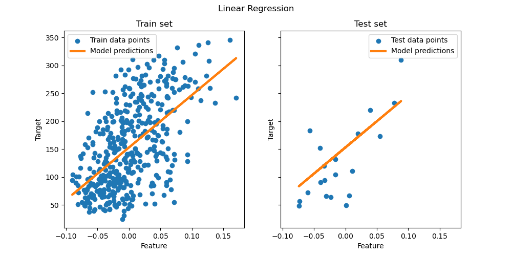](https://scikit-learn.org/stable/auto_examples/linear_model/plot_ols_ridge.html)
[`LinearRegression`](https://scikit-learn.org/stable/modules/generated/sklearn.linear_model.LinearRegression.html#sklearn.linear_model.LinearRegression "sklearn.linear_model.LinearRegression") takes in its `fit` method arguments `X`, `y`, `sample_weight` and stores the coefficients w of the linear model in its `coef_` and `intercept_` attributes:
```
>>> from sklearn import linear_model
>>> reg = linear_model.LinearRegression()
>>> reg.fit([[0, 0], [1, 1], [2, 2]], [0, 1, 2])
LinearRegression()
>>> reg.coef_
array([0.5, 0.5])
>>> reg.intercept_
0.0
```
The coefficient estimates for Ordinary Least Squares rely on the independence of the features. When features are correlated and some columns of the design matrix X have an approximately linear dependence, the design matrix becomes close to singular and as a result, the least-squares estimate becomes highly sensitive to random errors in the observed target, producing a large variance. This situation of *multicollinearity* can arise, for example, when data are collected without an experimental design.
Examples
- [Ordinary Least Squares and Ridge Regression](https://scikit-learn.org/stable/auto_examples/linear_model/plot_ols_ridge.html#sphx-glr-auto-examples-linear-model-plot-ols-ridge-py)
### 1\.1.1.1. Non-Negative Least Squares[\#](https://scikit-learn.org/stable/modules/linear_model.html#non-negative-least-squares "Link to this heading")
It is possible to constrain all the coefficients to be non-negative, which may be useful when they represent some physical or naturally non-negative quantities (e.g., frequency counts or prices of goods). [`LinearRegression`](https://scikit-learn.org/stable/modules/generated/sklearn.linear_model.LinearRegression.html#sklearn.linear_model.LinearRegression "sklearn.linear_model.LinearRegression") accepts a boolean `positive` parameter: when set to `True` [Non-Negative Least Squares](https://en.wikipedia.org/wiki/Non-negative_least_squares) are then applied.
Examples
- [Non-negative least squares](https://scikit-learn.org/stable/auto_examples/linear_model/plot_nnls.html#sphx-glr-auto-examples-linear-model-plot-nnls-py)
### 1\.1.1.2. Ordinary Least Squares Complexity[\#](https://scikit-learn.org/stable/modules/linear_model.html#ordinary-least-squares-complexity "Link to this heading")
The least squares solution is computed using the singular value decomposition of X. If X is a matrix of shape `(n_samples, n_features)` this method has a cost of O ( n samples n features 2 ), assuming that n samples ≥ n features.
## 1\.1.2. Ridge regression and classification[\#](https://scikit-learn.org/stable/modules/linear_model.html#ridge-regression-and-classification "Link to this heading")
### 1\.1.2.1. Regression[\#](https://scikit-learn.org/stable/modules/linear_model.html#regression "Link to this heading")
[`Ridge`](https://scikit-learn.org/stable/modules/generated/sklearn.linear_model.Ridge.html#sklearn.linear_model.Ridge "sklearn.linear_model.Ridge") regression addresses some of the problems of [Ordinary Least Squares](https://scikit-learn.org/stable/modules/linear_model.html#ordinary-least-squares) by imposing a penalty on the size of the coefficients. The ridge coefficients minimize a penalized residual sum of squares:
min
w
\|
\|
X
w
−
y
\|
\|
2
2
\+
α
\|
\|
w
\|
\|
2
2
The complexity parameter α ≥ 0 controls the amount of shrinkage: the larger the value of α, the greater the amount of shrinkage and thus the coefficients become more robust to collinearity.
[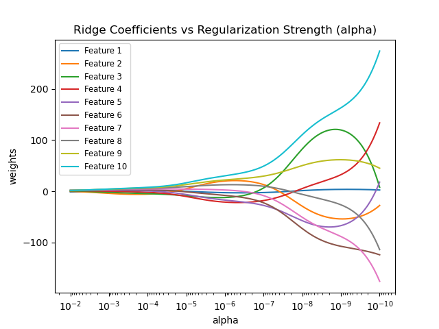](https://scikit-learn.org/stable/auto_examples/linear_model/plot_ridge_path.html)
As with other linear models, [`Ridge`](https://scikit-learn.org/stable/modules/generated/sklearn.linear_model.Ridge.html#sklearn.linear_model.Ridge "sklearn.linear_model.Ridge") will take in its `fit` method arrays `X`, `y` and will store the coefficients w of the linear model in its `coef_` member:
```
>>> from sklearn import linear_model
>>> reg = linear_model.Ridge(alpha=.5)
>>> reg.fit([[0, 0], [0, 0], [1, 1]], [0, .1, 1])
Ridge(alpha=0.5)
>>> reg.coef_
array([0.34545455, 0.34545455])
>>> reg.intercept_
np.float64(0.13636)
```
Note that the class [`Ridge`](https://scikit-learn.org/stable/modules/generated/sklearn.linear_model.Ridge.html#sklearn.linear_model.Ridge "sklearn.linear_model.Ridge") allows for the user to specify that the solver be automatically chosen by setting `solver="auto"`. When this option is specified, [`Ridge`](https://scikit-learn.org/stable/modules/generated/sklearn.linear_model.Ridge.html#sklearn.linear_model.Ridge "sklearn.linear_model.Ridge") will choose between the `"lbfgs"`, `"cholesky"`, and `"sparse_cg"` solvers. [`Ridge`](https://scikit-learn.org/stable/modules/generated/sklearn.linear_model.Ridge.html#sklearn.linear_model.Ridge "sklearn.linear_model.Ridge") will begin checking the conditions shown in the following table from top to bottom. If the condition is true, the corresponding solver is chosen.
| | |
|---|---|
| **Solver** | **Condition** |
| ‘lbfgs’ | The `positive=True` option is specified. |
| ‘cholesky’ | The input array X is not sparse. |
| ‘sparse\_cg’ | None of the above conditions are fulfilled. |
Examples
- [Ordinary Least Squares and Ridge Regression](https://scikit-learn.org/stable/auto_examples/linear_model/plot_ols_ridge.html#sphx-glr-auto-examples-linear-model-plot-ols-ridge-py)
- [Plot Ridge coefficients as a function of the regularization](https://scikit-learn.org/stable/auto_examples/linear_model/plot_ridge_path.html#sphx-glr-auto-examples-linear-model-plot-ridge-path-py)
- [Common pitfalls in the interpretation of coefficients of linear models](https://scikit-learn.org/stable/auto_examples/inspection/plot_linear_model_coefficient_interpretation.html#sphx-glr-auto-examples-inspection-plot-linear-model-coefficient-interpretation-py)
- [Ridge coefficients as a function of the L2 Regularization](https://scikit-learn.org/stable/auto_examples/linear_model/plot_ridge_coeffs.html#sphx-glr-auto-examples-linear-model-plot-ridge-coeffs-py)
### 1\.1.2.2. Classification[\#](https://scikit-learn.org/stable/modules/linear_model.html#classification "Link to this heading")
The [`Ridge`](https://scikit-learn.org/stable/modules/generated/sklearn.linear_model.Ridge.html#sklearn.linear_model.Ridge "sklearn.linear_model.Ridge") regressor has a classifier variant: [`RidgeClassifier`](https://scikit-learn.org/stable/modules/generated/sklearn.linear_model.RidgeClassifier.html#sklearn.linear_model.RidgeClassifier "sklearn.linear_model.RidgeClassifier"). This classifier first converts binary targets to `{-1, 1}` and then treats the problem as a regression task, optimizing the same objective as above. The predicted class corresponds to the sign of the regressor’s prediction. For multiclass classification, the problem is treated as multi-output regression, and the predicted class corresponds to the output with the highest value.
It might seem questionable to use a (penalized) Least Squares loss to fit a classification model instead of the more traditional logistic or hinge losses. However, in practice, all those models can lead to similar cross-validation scores in terms of accuracy or precision/recall, while the penalized least squares loss used by the [`RidgeClassifier`](https://scikit-learn.org/stable/modules/generated/sklearn.linear_model.RidgeClassifier.html#sklearn.linear_model.RidgeClassifier "sklearn.linear_model.RidgeClassifier") allows for a very different choice of the numerical solvers with distinct computational performance profiles.
The [`RidgeClassifier`](https://scikit-learn.org/stable/modules/generated/sklearn.linear_model.RidgeClassifier.html#sklearn.linear_model.RidgeClassifier "sklearn.linear_model.RidgeClassifier") can be significantly faster than e.g. [`LogisticRegression`](https://scikit-learn.org/stable/modules/generated/sklearn.linear_model.LogisticRegression.html#sklearn.linear_model.LogisticRegression "sklearn.linear_model.LogisticRegression") with a high number of classes because it can compute the projection matrix ( X T X ) − 1 X T only once.
This classifier is sometimes referred to as a [Least Squares Support Vector Machine](https://en.wikipedia.org/wiki/Least-squares_support-vector_machine) with a linear kernel.
Examples
- [Classification of text documents using sparse features](https://scikit-learn.org/stable/auto_examples/text/plot_document_classification_20newsgroups.html#sphx-glr-auto-examples-text-plot-document-classification-20newsgroups-py)
### 1\.1.2.3. Ridge Complexity[\#](https://scikit-learn.org/stable/modules/linear_model.html#ridge-complexity "Link to this heading")
This method has the same order of complexity as [Ordinary Least Squares](https://scikit-learn.org/stable/modules/linear_model.html#ordinary-least-squares).
### 1\.1.2.4. Setting the regularization parameter: leave-one-out Cross-Validation[\#](https://scikit-learn.org/stable/modules/linear_model.html#setting-the-regularization-parameter-leave-one-out-cross-validation "Link to this heading")
[`RidgeCV`](https://scikit-learn.org/stable/modules/generated/sklearn.linear_model.RidgeCV.html#sklearn.linear_model.RidgeCV "sklearn.linear_model.RidgeCV") and [`RidgeClassifierCV`](https://scikit-learn.org/stable/modules/generated/sklearn.linear_model.RidgeClassifierCV.html#sklearn.linear_model.RidgeClassifierCV "sklearn.linear_model.RidgeClassifierCV") implement ridge regression/classification with built-in cross-validation of the alpha parameter. They work in the same way as [`GridSearchCV`](https://scikit-learn.org/stable/modules/generated/sklearn.model_selection.GridSearchCV.html#sklearn.model_selection.GridSearchCV "sklearn.model_selection.GridSearchCV") except that it defaults to efficient Leave-One-Out [cross-validation](https://scikit-learn.org/stable/glossary.html#term-cross-validation). When using the default [cross-validation](https://scikit-learn.org/stable/glossary.html#term-cross-validation), alpha cannot be 0 due to the formulation used to calculate Leave-One-Out error. See [\[RL2007\]](https://scikit-learn.org/stable/modules/linear_model.html#rl2007) for details.
Usage example:
```
>>> import numpy as np
>>> from sklearn import linear_model
>>> reg = linear_model.RidgeCV(alphas=np.logspace(-6, 6, 13))
>>> reg.fit([[0, 0], [0, 0], [1, 1]], [0, .1, 1])
RidgeCV(alphas=array([1.e-06, 1.e-05, 1.e-04, 1.e-03, 1.e-02, 1.e-01, 1.e+00, 1.e+01,
1.e+02, 1.e+03, 1.e+04, 1.e+05, 1.e+06]))
>>> reg.alpha_
np.float64(0.01)
```
Specifying the value of the [cv](https://scikit-learn.org/stable/glossary.html#term-cv) attribute will trigger the use of cross-validation with [`GridSearchCV`](https://scikit-learn.org/stable/modules/generated/sklearn.model_selection.GridSearchCV.html#sklearn.model_selection.GridSearchCV "sklearn.model_selection.GridSearchCV"), for example `cv=10` for 10-fold cross-validation, rather than Leave-One-Out Cross-Validation.
References[\#](https://scikit-learn.org/stable/modules/linear_model.html#references "Link to this dropdown")
\[[RL2007](https://scikit-learn.org/stable/modules/linear_model.html#id3)\]
“Notes on Regularized Least Squares”, Rifkin & Lippert ([technical report](http://cbcl.mit.edu/publications/ps/MIT-CSAIL-TR-2007-025.pdf), [course slides](https://www.mit.edu/~9.520/spring07/Classes/rlsslides.pdf)).
## 1\.1.3. Lasso[\#](https://scikit-learn.org/stable/modules/linear_model.html#lasso "Link to this heading")
The [`Lasso`](https://scikit-learn.org/stable/modules/generated/sklearn.linear_model.Lasso.html#sklearn.linear_model.Lasso "sklearn.linear_model.Lasso") is a linear model that estimates sparse coefficients, i.e., it is able to set coefficients exactly to zero. It is useful in some contexts due to its tendency to prefer solutions with fewer non-zero coefficients, effectively reducing the number of features upon which the given solution is dependent. For this reason, Lasso and its variants are fundamental to the field of compressed sensing. Under certain conditions, it can recover the exact set of non-zero coefficients (see [Compressive sensing: tomography reconstruction with L1 prior (Lasso)](https://scikit-learn.org/stable/auto_examples/applications/plot_tomography_l1_reconstruction.html#sphx-glr-auto-examples-applications-plot-tomography-l1-reconstruction-py)).
Mathematically, it consists of a linear model with an added regularization term. The objective function to minimize is:
min
w
P
(
w
)
\=
1
2
n
samples
\|
\|
X
w
−
y
\|
\|
2
2
\+
α
\|
\|
w
\|
\|
1
The lasso estimate thus solves the least-squares with added penalty α \| \| w \| \| 1, where α is a constant and \| \| w \| \| 1 is the ℓ 1\-norm of the coefficient vector.
The implementation in the class [`Lasso`](https://scikit-learn.org/stable/modules/generated/sklearn.linear_model.Lasso.html#sklearn.linear_model.Lasso "sklearn.linear_model.Lasso") uses coordinate descent as the algorithm to fit the coefficients. See [Least Angle Regression](https://scikit-learn.org/stable/modules/linear_model.html#least-angle-regression) for another implementation:
```
>>> from sklearn import linear_model
>>> reg = linear_model.Lasso(alpha=0.1)
>>> reg.fit([[0, 0], [1, 1]], [0, 1])
Lasso(alpha=0.1)
>>> reg.predict([[1, 1]])
array([0.8])
```
The function [`lasso_path`](https://scikit-learn.org/stable/modules/generated/sklearn.linear_model.lasso_path.html#sklearn.linear_model.lasso_path "sklearn.linear_model.lasso_path") is useful for lower-level tasks, as it computes the coefficients along the full path of possible values.
Examples
- [L1-based models for Sparse Signals](https://scikit-learn.org/stable/auto_examples/linear_model/plot_lasso_and_elasticnet.html#sphx-glr-auto-examples-linear-model-plot-lasso-and-elasticnet-py)
- [Compressive sensing: tomography reconstruction with L1 prior (Lasso)](https://scikit-learn.org/stable/auto_examples/applications/plot_tomography_l1_reconstruction.html#sphx-glr-auto-examples-applications-plot-tomography-l1-reconstruction-py)
- [Common pitfalls in the interpretation of coefficients of linear models](https://scikit-learn.org/stable/auto_examples/inspection/plot_linear_model_coefficient_interpretation.html#sphx-glr-auto-examples-inspection-plot-linear-model-coefficient-interpretation-py)
- [Lasso model selection: AIC-BIC / cross-validation](https://scikit-learn.org/stable/auto_examples/linear_model/plot_lasso_model_selection.html#sphx-glr-auto-examples-linear-model-plot-lasso-model-selection-py)
Note
**Feature selection with Lasso**
As the Lasso regression yields sparse models, it can thus be used to perform feature selection, as detailed in [L1-based feature selection](https://scikit-learn.org/stable/modules/feature_selection.html#l1-feature-selection).
References[\#](https://scikit-learn.org/stable/modules/linear_model.html#references-2 "Link to this dropdown")
The following references explain the origin of the Lasso as well as properties of the Lasso problem and the duality gap computation used for convergence control.
- [Robert Tibshirani. (1996) Regression Shrinkage and Selection Via the Lasso. J. R. Stat. Soc. Ser. B Stat. Methodol., 58(1):267-288](https://doi.org/10.1111/j.2517-6161.1996.tb02080.x)
- “An Interior-Point Method for Large-Scale L1-Regularized Least Squares,” S. J. Kim, K. Koh, M. Lustig, S. Boyd and D. Gorinevsky, in IEEE Journal of Selected Topics in Signal Processing, 2007 ([Paper](https://web.stanford.edu/~boyd/papers/pdf/l1_ls.pdf))
### 1\.1.3.1. Coordinate Descent with Gap Safe Screening Rules[\#](https://scikit-learn.org/stable/modules/linear_model.html#coordinate-descent-with-gap-safe-screening-rules "Link to this heading")
Coordinate descent (CD) is a strategy to solve a minimization problem that considers a single feature j at a time. This way, the optimization problem is reduced to a 1-dimensional problem which is easier to solve:
min
w
j
1
2
n
samples
\|
\|
x
j
w
j
\+
X
−
j
w
−
j
−
y
\|
\|
2
2
\+
α
\|
w
j
\|
with index − j meaning all features but j. The solution is
w
j
\=
S
(
x
j
T
(
y
−
X
−
j
w
−
j
)
,
α
)
\|
\|
x
j
\|
\|
2
2
with the soft-thresholding function S ( z , α ) \= sign ( z ) max ( 0 , \| z \| − α ). Note that the soft-thresholding function is exactly zero whenever α ≥ \| z \|. The CD solver then loops over the features either in a cycle, picking one feature after the other in the order given by `X` (`selection="cyclic"`), or by randomly picking features (`selection="random"`). It stops if the duality gap is smaller than the provided tolerance `tol`.
Mathematical details[\#](https://scikit-learn.org/stable/modules/linear_model.html#mathematical-details "Link to this dropdown")
The duality gap G ( w , v ) is an upper bound of the difference between the current primal objective function of the Lasso, P ( w ), and its minimum P ( w ⋆ ), i.e. G ( w , v ) ≥ P ( w ) − P ( w ⋆ ). It is given by G ( w , v ) \= P ( w ) − D ( v ) with dual objective function
D
(
v
)
\=
1
2
n
samples
(
y
T
v
−
\|
\|
v
\|
\|
2
2
)
subject to v ∈ \| \| X T v \| \| ∞ ≤ n samples α. At optimum, the duality gap is zero, G ( w ⋆ , v ⋆ ) \= 0 (a property called strong duality). With (scaled) dual variable v \= c r, current residual r \= y − X w and dual scaling
c
\=
{
1
,
\|
\|
X
T
r
\|
\|
∞
≤
n
samples
α
,
n
samples
α
\|
\|
X
T
r
\|
\|
∞
,
otherwise
the stopping criterion is
tol
\|
\|
y
\|
\|
2
2
n
samples
\<
G
(
w
,
c
r
)
.
A clever method to speedup the coordinate descent algorithm is to screen features such that at optimum w j \= 0. Gap safe screening rules are such a tool. Anywhere during the optimization algorithm, they can tell which feature we can safely exclude, i.e., set to zero with certainty.
References[\#](https://scikit-learn.org/stable/modules/linear_model.html#references-3 "Link to this dropdown")
The first reference explains the coordinate descent solver used in scikit-learn, the others treat gap safe screening rules.
- [Friedman, Hastie & Tibshirani. (2010). Regularization Path For Generalized linear Models by Coordinate Descent. J Stat Softw 33(1), 1-22](https://doi.org/10.18637/jss.v033.i01)
- [O. Fercoq, A. Gramfort, J. Salmon. (2015). Mind the duality gap: safer rules for the Lasso. Proceedings of Machine Learning Research 37:333-342, 2015.](https://arxiv.org/abs/1505.03410)
- [E. Ndiaye, O. Fercoq, A. Gramfort, J. Salmon. (2017). Gap Safe Screening Rules for Sparsity Enforcing Penalties. Journal of Machine Learning Research 18(128):1-33, 2017.](https://arxiv.org/abs/1611.05780)
### 1\.1.3.2. Setting regularization parameter[\#](https://scikit-learn.org/stable/modules/linear_model.html#setting-regularization-parameter "Link to this heading")
The `alpha` parameter controls the degree of sparsity of the estimated coefficients.
#### 1\.1.3.2.1. Using cross-validation[\#](https://scikit-learn.org/stable/modules/linear_model.html#using-cross-validation "Link to this heading")
scikit-learn exposes objects that set the Lasso `alpha` parameter by cross-validation: [`LassoCV`](https://scikit-learn.org/stable/modules/generated/sklearn.linear_model.LassoCV.html#sklearn.linear_model.LassoCV "sklearn.linear_model.LassoCV") and [`LassoLarsCV`](https://scikit-learn.org/stable/modules/generated/sklearn.linear_model.LassoLarsCV.html#sklearn.linear_model.LassoLarsCV "sklearn.linear_model.LassoLarsCV"). [`LassoLarsCV`](https://scikit-learn.org/stable/modules/generated/sklearn.linear_model.LassoLarsCV.html#sklearn.linear_model.LassoLarsCV "sklearn.linear_model.LassoLarsCV") is based on the [Least Angle Regression](https://scikit-learn.org/stable/modules/linear_model.html#least-angle-regression) algorithm explained below.
For high-dimensional datasets with many collinear features, [`LassoCV`](https://scikit-learn.org/stable/modules/generated/sklearn.linear_model.LassoCV.html#sklearn.linear_model.LassoCV "sklearn.linear_model.LassoCV") is most often preferable. However, [`LassoLarsCV`](https://scikit-learn.org/stable/modules/generated/sklearn.linear_model.LassoLarsCV.html#sklearn.linear_model.LassoLarsCV "sklearn.linear_model.LassoLarsCV") has the advantage of exploring more relevant values of `alpha` parameter, and if the number of samples is very small compared to the number of features, it is often faster than [`LassoCV`](https://scikit-learn.org/stable/modules/generated/sklearn.linear_model.LassoCV.html#sklearn.linear_model.LassoCV "sklearn.linear_model.LassoCV").
**[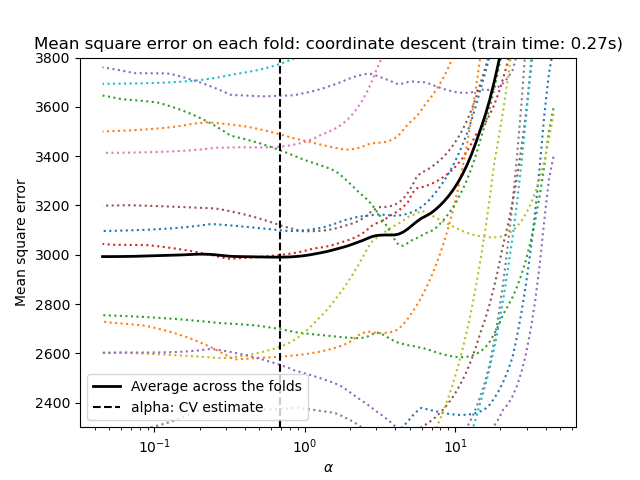](https://scikit-learn.org/stable/auto_examples/linear_model/plot_lasso_model_selection.html) [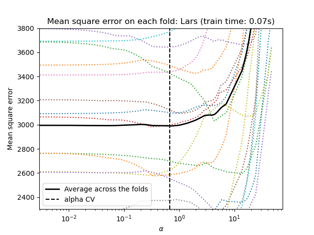](https://scikit-learn.org/stable/auto_examples/linear_model/plot_lasso_model_selection.html)**
#### 1\.1.3.2.2. Information-criteria based model selection[\#](https://scikit-learn.org/stable/modules/linear_model.html#information-criteria-based-model-selection "Link to this heading")
Alternatively, the estimator [`LassoLarsIC`](https://scikit-learn.org/stable/modules/generated/sklearn.linear_model.LassoLarsIC.html#sklearn.linear_model.LassoLarsIC "sklearn.linear_model.LassoLarsIC") proposes to use the Akaike information criterion (AIC) and the Bayes Information criterion (BIC). It is a computationally cheaper alternative to find the optimal value of alpha as the regularization path is computed only once instead of k+1 times when using k-fold cross-validation.
Indeed, these criteria are computed on the in-sample training set. In short, they penalize the over-optimistic scores of the different Lasso models by their flexibility (cf. to “Mathematical details” section below).
However, such criteria need a proper estimation of the degrees of freedom of the solution, are derived for large samples (asymptotic results) and assume the correct model is candidates under investigation. They also tend to break when the problem is badly conditioned (e.g. more features than samples).
[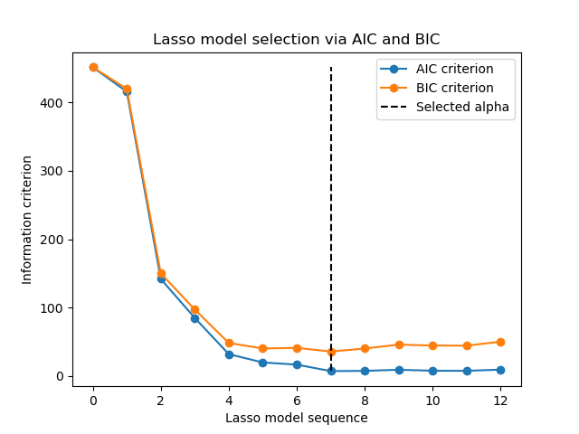](https://scikit-learn.org/stable/auto_examples/linear_model/plot_lasso_lars_ic.html)
Examples
- [Lasso model selection: AIC-BIC / cross-validation](https://scikit-learn.org/stable/auto_examples/linear_model/plot_lasso_model_selection.html#sphx-glr-auto-examples-linear-model-plot-lasso-model-selection-py)
- [Lasso model selection via information criteria](https://scikit-learn.org/stable/auto_examples/linear_model/plot_lasso_lars_ic.html#sphx-glr-auto-examples-linear-model-plot-lasso-lars-ic-py)
#### 1\.1.3.2.3. AIC and BIC criteria[\#](https://scikit-learn.org/stable/modules/linear_model.html#aic-and-bic-criteria "Link to this heading")
The definition of AIC (and thus BIC) might differ in the literature. In this section, we give more information regarding the criterion computed in scikit-learn.
Mathematical details[\#](https://scikit-learn.org/stable/modules/linear_model.html#mathematical-details-2 "Link to this dropdown")
The AIC criterion is defined as:
A
I
C
\=
−
2
log
(
L
^
)
\+
2
d
where L ^ is the maximum likelihood of the model and d is the number of parameters (as well referred to as degrees of freedom in the previous section).
The definition of BIC replaces the constant 2 by log ( N ):
B
I
C
\=
−
2
log
(
L
^
)
\+
log
(
N
)
d
where N is the number of samples.
For a linear Gaussian model, the maximum log-likelihood is defined as:
log
(
L
^
)
\=
−
n
2
log
(
2
π
)
−
n
2
log
(
σ
2
)
−
∑
i
\=
1
n
(
y
i
−
y
^
i
)
2
2
σ
2
where σ 2 is an estimate of the noise variance, y i and y ^ i are respectively the true and predicted targets, and n is the number of samples.
Plugging the maximum log-likelihood in the AIC formula yields:
A
I
C
\=
n
log
(
2
π
σ
2
)
\+
∑
i
\=
1
n
(
y
i
−
y
^
i
)
2
σ
2
\+
2
d
The first term of the above expression is sometimes discarded since it is a constant when σ 2 is provided. In addition, it is sometimes stated that the AIC is equivalent to the C p statistic [\[12\]](https://scikit-learn.org/stable/modules/linear_model.html#id7). In a strict sense, however, it is equivalent only up to some constant and a multiplicative factor.
At last, we mentioned above that σ 2 is an estimate of the noise variance. In [`LassoLarsIC`](https://scikit-learn.org/stable/modules/generated/sklearn.linear_model.LassoLarsIC.html#sklearn.linear_model.LassoLarsIC "sklearn.linear_model.LassoLarsIC") when the parameter `noise_variance` is not provided (default), the noise variance is estimated via the unbiased estimator [\[13\]](https://scikit-learn.org/stable/modules/linear_model.html#id8) defined as:
σ
2
\=
∑
i
\=
1
n
(
y
i
−
y
^
i
)
2
n
−
p
where p is the number of features and y ^ i is the predicted target using an ordinary least squares regression. Note, that this formula is valid only when `n_samples > n_features`.
References
\[[12](https://scikit-learn.org/stable/modules/linear_model.html#id5)\]
[Zou, Hui, Trevor Hastie, and Robert Tibshirani. “On the degrees of freedom of the lasso.” The Annals of Statistics 35.5 (2007): 2173-2192.](https://arxiv.org/abs/0712.0881.pdf)
\[[13](https://scikit-learn.org/stable/modules/linear_model.html#id6)\]
[Cherkassky, Vladimir, and Yunqian Ma. “Comparison of model selection for regression.” Neural computation 15.7 (2003): 1691-1714.](https://doi.org/10.1162/089976603321891864)
#### 1\.1.3.2.4. Comparison with the regularization parameter of SVM[\#](https://scikit-learn.org/stable/modules/linear_model.html#comparison-with-the-regularization-parameter-of-svm "Link to this heading")
The equivalence between `alpha` and the regularization parameter of SVM, `C` is given by `alpha = 1 / C` or `alpha = 1 / (n_samples * C)`, depending on the estimator and the exact objective function optimized by the model.
## 1\.1.4. Multi-task Lasso[\#](https://scikit-learn.org/stable/modules/linear_model.html#multi-task-lasso "Link to this heading")
The [`MultiTaskLasso`](https://scikit-learn.org/stable/modules/generated/sklearn.linear_model.MultiTaskLasso.html#sklearn.linear_model.MultiTaskLasso "sklearn.linear_model.MultiTaskLasso") is a linear model that estimates sparse coefficients for multiple regression problems jointly: `y` is a 2D array, of shape `(n_samples, n_tasks)`. The constraint is that the selected features are the same for all the regression problems, also called tasks.
The following figure compares the location of the non-zero entries in the coefficient matrix W obtained with a simple Lasso or a MultiTaskLasso. The Lasso estimates yield scattered non-zeros while the non-zeros of the MultiTaskLasso are full columns.
**[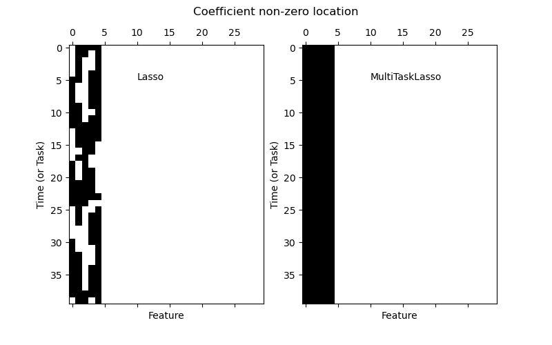](https://scikit-learn.org/stable/auto_examples/linear_model/plot_multi_task_lasso_support.html) [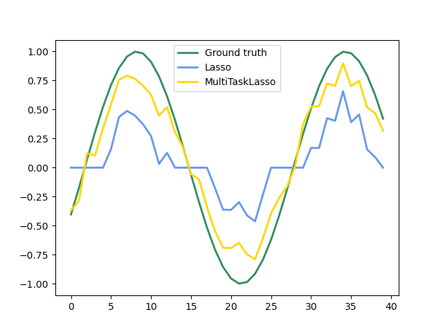](https://scikit-learn.org/stable/auto_examples/linear_model/plot_multi_task_lasso_support.html)**
**Fitting a time-series model, imposing that any active feature be active at all times.**
Examples
- [Joint feature selection with multi-task Lasso](https://scikit-learn.org/stable/auto_examples/linear_model/plot_multi_task_lasso_support.html#sphx-glr-auto-examples-linear-model-plot-multi-task-lasso-support-py)
Mathematical details[\#](https://scikit-learn.org/stable/modules/linear_model.html#mathematical-details-3 "Link to this dropdown")
Mathematically, it consists of a linear model trained with a mixed ℓ 1 ℓ 2\-norm for regularization. The objective function to minimize is:
min
W
1
2
n
samples
\|
\|
X
W
−
Y
\|
\|
Fro
2
\+
α
\|
\|
W
\|
\|
21
where Fro indicates the Frobenius norm
\|
\|
A
\|
\|
Fro
\=
∑
i
j
a
i
j
2
and ℓ 1 ℓ 2 reads
\|
\|
A
\|
\|
2
1
\=
∑
i
∑
j
a
i
j
2
.
The implementation in the class [`MultiTaskLasso`](https://scikit-learn.org/stable/modules/generated/sklearn.linear_model.MultiTaskLasso.html#sklearn.linear_model.MultiTaskLasso "sklearn.linear_model.MultiTaskLasso") uses coordinate descent as the algorithm to fit the coefficients.
## 1\.1.5. Elastic-Net[\#](https://scikit-learn.org/stable/modules/linear_model.html#elastic-net "Link to this heading")
[`ElasticNet`](https://scikit-learn.org/stable/modules/generated/sklearn.linear_model.ElasticNet.html#sklearn.linear_model.ElasticNet "sklearn.linear_model.ElasticNet") is a linear regression model trained with both ℓ 1 and ℓ 2\-norm regularization of the coefficients. This combination allows for learning a sparse model where few of the weights are non-zero like [`Lasso`](https://scikit-learn.org/stable/modules/generated/sklearn.linear_model.Lasso.html#sklearn.linear_model.Lasso "sklearn.linear_model.Lasso"), while still maintaining the regularization properties of [`Ridge`](https://scikit-learn.org/stable/modules/generated/sklearn.linear_model.Ridge.html#sklearn.linear_model.Ridge "sklearn.linear_model.Ridge"). We control the convex combination of ℓ 1 and ℓ 2 using the `l1_ratio` parameter.
Elastic-net is useful when there are multiple features that are correlated with one another. Lasso is likely to pick one of these at random, while elastic-net is likely to pick both.
A practical advantage of trading-off between Lasso and Ridge is that it allows Elastic-Net to inherit some of Ridge’s stability under rotation.
The objective function to minimize is in this case
min
w
1
2
n
samples
\|
\|
X
w
−
y
\|
\|
2
2
\+
α
ρ
\|
\|
w
\|
\|
1
\+
α
(
1
−
ρ
)
2
\|
\|
w
\|
\|
2
2
[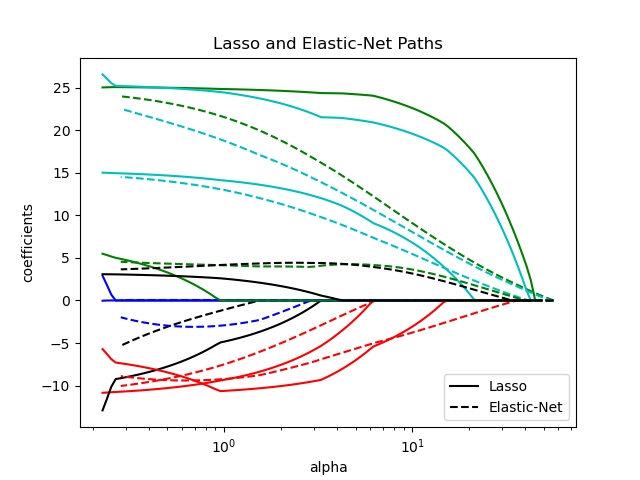](https://scikit-learn.org/stable/auto_examples/linear_model/plot_lasso_lasso_lars_elasticnet_path.html)
The class [`ElasticNetCV`](https://scikit-learn.org/stable/modules/generated/sklearn.linear_model.ElasticNetCV.html#sklearn.linear_model.ElasticNetCV "sklearn.linear_model.ElasticNetCV") can be used to set the parameters `alpha` (α) and `l1_ratio` (ρ) by cross-validation.
Examples
- [L1-based models for Sparse Signals](https://scikit-learn.org/stable/auto_examples/linear_model/plot_lasso_and_elasticnet.html#sphx-glr-auto-examples-linear-model-plot-lasso-and-elasticnet-py)
- [Lasso, Lasso-LARS, and Elastic Net paths](https://scikit-learn.org/stable/auto_examples/linear_model/plot_lasso_lasso_lars_elasticnet_path.html#sphx-glr-auto-examples-linear-model-plot-lasso-lasso-lars-elasticnet-path-py)
- [Fitting an Elastic Net with a precomputed Gram Matrix and Weighted Samples](https://scikit-learn.org/stable/auto_examples/linear_model/plot_elastic_net_precomputed_gram_matrix_with_weighted_samples.html#sphx-glr-auto-examples-linear-model-plot-elastic-net-precomputed-gram-matrix-with-weighted-samples-py)
References[\#](https://scikit-learn.org/stable/modules/linear_model.html#references-4 "Link to this dropdown")
The following two references explain the iterations used in the coordinate descent solver of scikit-learn, as well as the duality gap computation used for convergence control.
- “Regularization Path For Generalized linear Models by Coordinate Descent”, Friedman, Hastie & Tibshirani, J Stat Softw, 2010 ([Paper](https://www.jstatsoft.org/article/view/v033i01/v33i01.pdf)).
- “An Interior-Point Method for Large-Scale L1-Regularized Least Squares,” S. J. Kim, K. Koh, M. Lustig, S. Boyd and D. Gorinevsky, in IEEE Journal of Selected Topics in Signal Processing, 2007 ([Paper](https://web.stanford.edu/~boyd/papers/pdf/l1_ls.pdf))
## 1\.1.6. Multi-task Elastic-Net[\#](https://scikit-learn.org/stable/modules/linear_model.html#multi-task-elastic-net "Link to this heading")
The [`MultiTaskElasticNet`](https://scikit-learn.org/stable/modules/generated/sklearn.linear_model.MultiTaskElasticNet.html#sklearn.linear_model.MultiTaskElasticNet "sklearn.linear_model.MultiTaskElasticNet") is an elastic-net model that estimates sparse coefficients for multiple regression problems jointly: `Y` is a 2D array of shape `(n_samples, n_tasks)`. The constraint is that the selected features are the same for all the regression problems, also called tasks.
Mathematically, it consists of a linear model trained with a mixed ℓ 1 ℓ 2\-norm and ℓ 2\-norm for regularization. The objective function to minimize is:
min
W
1
2
n
samples
\|
\|
X
W
−
Y
\|
\|
Fro
2
\+
α
ρ
\|
\|
W
\|
\|
2
1
\+
α
(
1
−
ρ
)
2
\|
\|
W
\|
\|
Fro
2
The implementation in the class [`MultiTaskElasticNet`](https://scikit-learn.org/stable/modules/generated/sklearn.linear_model.MultiTaskElasticNet.html#sklearn.linear_model.MultiTaskElasticNet "sklearn.linear_model.MultiTaskElasticNet") uses coordinate descent as the algorithm to fit the coefficients.
The class [`MultiTaskElasticNetCV`](https://scikit-learn.org/stable/modules/generated/sklearn.linear_model.MultiTaskElasticNetCV.html#sklearn.linear_model.MultiTaskElasticNetCV "sklearn.linear_model.MultiTaskElasticNetCV") can be used to set the parameters `alpha` (α) and `l1_ratio` (ρ) by cross-validation.
## 1\.1.7. Least Angle Regression[\#](https://scikit-learn.org/stable/modules/linear_model.html#least-angle-regression "Link to this heading")
Least-angle regression (LARS) is a regression algorithm for high-dimensional data, developed by Bradley Efron, Trevor Hastie, Iain Johnstone and Robert Tibshirani. LARS is similar to forward stepwise regression. At each step, it finds the feature most correlated with the target. When there are multiple features having equal correlation, instead of continuing along the same feature, it proceeds in a direction equiangular between the features.
The advantages of LARS are:
- It is numerically efficient in contexts where the number of features is significantly greater than the number of samples.
- It is computationally just as fast as forward selection and has the same order of complexity as ordinary least squares.
- It produces a full piecewise linear solution path, which is useful in cross-validation or similar attempts to tune the model.
- If two features are almost equally correlated with the target, then their coefficients should increase at approximately the same rate. The algorithm thus behaves as intuition would expect, and also is more stable.
- It is easily modified to produce solutions for other estimators, like the Lasso.
The disadvantages of the LARS method include:
- Because LARS is based upon an iterative refitting of the residuals, it would appear to be especially sensitive to the effects of noise. This problem is discussed in detail by Weisberg in the discussion section of the Efron et al. (2004) Annals of Statistics article.
The LARS model can be used via the estimator [`Lars`](https://scikit-learn.org/stable/modules/generated/sklearn.linear_model.Lars.html#sklearn.linear_model.Lars "sklearn.linear_model.Lars"), or its low-level implementation [`lars_path`](https://scikit-learn.org/stable/modules/generated/sklearn.linear_model.lars_path.html#sklearn.linear_model.lars_path "sklearn.linear_model.lars_path") or [`lars_path_gram`](https://scikit-learn.org/stable/modules/generated/sklearn.linear_model.lars_path_gram.html#sklearn.linear_model.lars_path_gram "sklearn.linear_model.lars_path_gram").
## 1\.1.8. LARS Lasso[\#](https://scikit-learn.org/stable/modules/linear_model.html#lars-lasso "Link to this heading")
[`LassoLars`](https://scikit-learn.org/stable/modules/generated/sklearn.linear_model.LassoLars.html#sklearn.linear_model.LassoLars "sklearn.linear_model.LassoLars") is a lasso model implemented using the LARS algorithm, and unlike the implementation based on coordinate descent, this yields the exact solution, which is piecewise linear as a function of the norm of its coefficients.
[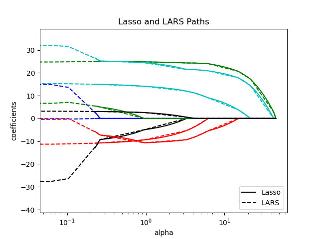](https://scikit-learn.org/stable/auto_examples/linear_model/plot_lasso_lasso_lars_elasticnet_path.html)
```
>>> from sklearn import linear_model
>>> reg = linear_model.LassoLars(alpha=.1)
>>> reg.fit([[0, 0], [1, 1]], [0, 1])
LassoLars(alpha=0.1)
>>> reg.coef_
array([0.6, 0. ])
```
Examples
- [Lasso, Lasso-LARS, and Elastic Net paths](https://scikit-learn.org/stable/auto_examples/linear_model/plot_lasso_lasso_lars_elasticnet_path.html#sphx-glr-auto-examples-linear-model-plot-lasso-lasso-lars-elasticnet-path-py)
The LARS algorithm provides the full path of the coefficients along the regularization parameter almost for free, thus a common operation is to retrieve the path with one of the functions [`lars_path`](https://scikit-learn.org/stable/modules/generated/sklearn.linear_model.lars_path.html#sklearn.linear_model.lars_path "sklearn.linear_model.lars_path") or [`lars_path_gram`](https://scikit-learn.org/stable/modules/generated/sklearn.linear_model.lars_path_gram.html#sklearn.linear_model.lars_path_gram "sklearn.linear_model.lars_path_gram").
Mathematical formulation[\#](https://scikit-learn.org/stable/modules/linear_model.html#mathematical-formulation "Link to this dropdown")
The algorithm is similar to forward stepwise regression, but instead of including features at each step, the estimated coefficients are increased in a direction equiangular to each one’s correlations with the residual.
Instead of giving a vector result, the LARS solution consists of a curve denoting the solution for each value of the ℓ 1 norm of the parameter vector. The full coefficients path is stored in the array `coef_path_` of shape `(n_features, max_features + 1)`. The first column is always zero.
References
- Original Algorithm is detailed in the paper [Least Angle Regression](https://hastie.su.domains/Papers/LARS/LeastAngle_2002.pdf) by Hastie et al.
## 1\.1.9. Orthogonal Matching Pursuit (OMP)[\#](https://scikit-learn.org/stable/modules/linear_model.html#orthogonal-matching-pursuit-omp "Link to this heading")
[`OrthogonalMatchingPursuit`](https://scikit-learn.org/stable/modules/generated/sklearn.linear_model.OrthogonalMatchingPursuit.html#sklearn.linear_model.OrthogonalMatchingPursuit "sklearn.linear_model.OrthogonalMatchingPursuit") and [`orthogonal_mp`](https://scikit-learn.org/stable/modules/generated/sklearn.linear_model.orthogonal_mp.html#sklearn.linear_model.orthogonal_mp "sklearn.linear_model.orthogonal_mp") implement the OMP algorithm for approximating the fit of a linear model with constraints imposed on the number of non-zero coefficients (i.e. the ℓ 0 pseudo-norm).
Being a forward feature selection method like [Least Angle Regression](https://scikit-learn.org/stable/modules/linear_model.html#least-angle-regression), orthogonal matching pursuit can approximate the optimum solution vector with a fixed number of non-zero elements:
arg
min
w
\|
\|
y
−
X
w
\|
\|
2
2
subject to
\|
\|
w
\|
\|
0
≤
n
nonzero\_coefs
Alternatively, orthogonal matching pursuit can target a specific error instead of a specific number of non-zero coefficients. This can be expressed as:
arg
min
w
\|
\|
w
\|
\|
0
subject to
\|
\|
y
−
X
w
\|
\|
2
2
≤
tol
OMP is based on a greedy algorithm that includes at each step the atom most highly correlated with the current residual. It is similar to the simpler matching pursuit (MP) method, but better in that at each iteration, the residual is recomputed using an orthogonal projection on the space of the previously chosen dictionary elements.
Examples
- [Orthogonal Matching Pursuit](https://scikit-learn.org/stable/auto_examples/linear_model/plot_omp.html#sphx-glr-auto-examples-linear-model-plot-omp-py)
References[\#](https://scikit-learn.org/stable/modules/linear_model.html#references-5 "Link to this dropdown")
- <https://www.cs.technion.ac.il/~ronrubin/Publications/KSVD-OMP-v2.pdf>
- [Matching pursuits with time-frequency dictionaries](https://www.di.ens.fr/~mallat/papiers/MallatPursuit93.pdf), S. G. Mallat, Z. Zhang, 1993.
## 1\.1.10. Bayesian Regression[\#](https://scikit-learn.org/stable/modules/linear_model.html#bayesian-regression "Link to this heading")
Bayesian regression techniques can be used to include regularization parameters in the estimation procedure: the regularization parameter is not set in a hard sense but tuned to the data at hand.
This can be done by introducing [uninformative priors](https://en.wikipedia.org/wiki/Non-informative_prior#Uninformative_priors) over the hyper parameters of the model. The ℓ 2 regularization used in [Ridge regression and classification](https://scikit-learn.org/stable/modules/linear_model.html#ridge-regression) is equivalent to finding a maximum a posteriori estimation under a Gaussian prior over the coefficients w with precision λ − 1. Instead of setting `lambda` manually, it is possible to treat it as a random variable to be estimated from the data.
To obtain a fully probabilistic model, the output y is assumed to be Gaussian distributed around X w:
p
(
y
\|
X
,
w
,
α
)
\=
N
(
y
\|
X
w
,
α
−
1
)
where α is again treated as a random variable that is to be estimated from the data.
The advantages of Bayesian Regression are:
- It adapts to the data at hand.
- It can be used to include regularization parameters in the estimation procedure.
The disadvantages of Bayesian regression include:
- Inference of the model can be time consuming.
References[\#](https://scikit-learn.org/stable/modules/linear_model.html#references-6 "Link to this dropdown")
- A good introduction to Bayesian methods is given in [C. Bishop: Pattern Recognition and Machine Learning](https://www.microsoft.com/en-us/research/wp-content/uploads/2006/01/Bishop-Pattern-Recognition-and-Machine-Learning-2006.pdf).
- Original Algorithm is detailed in the book [Bayesian learning for neural networks](https://citeseerx.ist.psu.edu/document?repid=rep1&type=pdf&doi=db869fa192a3222ae4f2d766674a378e47013b1b) by Radford M. Neal.
### 1\.1.10.1. Bayesian Ridge Regression[\#](https://scikit-learn.org/stable/modules/linear_model.html#bayesian-ridge-regression "Link to this heading")
[`BayesianRidge`](https://scikit-learn.org/stable/modules/generated/sklearn.linear_model.BayesianRidge.html#sklearn.linear_model.BayesianRidge "sklearn.linear_model.BayesianRidge") estimates a probabilistic model of the regression problem as described above. The prior for the coefficient w is given by a spherical Gaussian:
p
(
w
\|
λ
)
\=
N
(
w
\|
0
,
λ
−
1
I
p
)
The priors over α and λ are chosen to be [gamma distributions](https://en.wikipedia.org/wiki/Gamma_distribution), the conjugate prior for the precision of the Gaussian. The resulting model is called *Bayesian Ridge Regression*, and is similar to the classical [`Ridge`](https://scikit-learn.org/stable/modules/generated/sklearn.linear_model.Ridge.html#sklearn.linear_model.Ridge "sklearn.linear_model.Ridge").
The parameters w, α and λ are estimated jointly during the fit of the model, the regularization parameters α and λ being estimated by maximizing the *log marginal likelihood*. The scikit-learn implementation is based on the algorithm described in Appendix A of (Tipping, 2001) where the update of the parameters α and λ is done as suggested in (MacKay, 1992). The initial value of the maximization procedure can be set with the hyperparameters `alpha_init` and `lambda_init`.
There are four more hyperparameters, α 1, α 2, λ 1 and λ 2 of the gamma prior distributions over α and λ. These are usually chosen to be *non-informative*. By default α 1 \= α 2 \= λ 1 \= λ 2 \= 10 − 6.
Bayesian Ridge Regression is used for regression:
```
>>> from sklearn import linear_model
>>> X = [[0., 0.], [1., 1.], [2., 2.], [3., 3.]]
>>> Y = [0., 1., 2., 3.]
>>> reg = linear_model.BayesianRidge()
>>> reg.fit(X, Y)
BayesianRidge()
```
After being fitted, the model can then be used to predict new values:
```
>>> reg.predict([[1, 0.]])
array([0.50000013])
```
The coefficients w of the model can be accessed:
```
>>> reg.coef_
array([0.49999993, 0.49999993])
```
Due to the Bayesian framework, the weights found are slightly different from the ones found by [Ordinary Least Squares](https://scikit-learn.org/stable/modules/linear_model.html#ordinary-least-squares). However, Bayesian Ridge Regression is more robust to ill-posed problems.
Examples
- [Curve Fitting with Bayesian Ridge Regression](https://scikit-learn.org/stable/auto_examples/linear_model/plot_bayesian_ridge_curvefit.html#sphx-glr-auto-examples-linear-model-plot-bayesian-ridge-curvefit-py)
References[\#](https://scikit-learn.org/stable/modules/linear_model.html#references-7 "Link to this dropdown")
- Section 3.3 in Christopher M. Bishop: Pattern Recognition and Machine Learning, 2006
- David J. C. MacKay, [Bayesian Interpolation](https://citeseerx.ist.psu.edu/doc_view/pid/b14c7cc3686e82ba40653c6dff178356a33e5e2c), 1992.
- Michael E. Tipping, [Sparse Bayesian Learning and the Relevance Vector Machine](https://www.jmlr.org/papers/volume1/tipping01a/tipping01a.pdf), 2001.
### 1\.1.10.2. Automatic Relevance Determination - ARD[\#](https://scikit-learn.org/stable/modules/linear_model.html#automatic-relevance-determination-ard "Link to this heading")
The Automatic Relevance Determination (as being implemented in [`ARDRegression`](https://scikit-learn.org/stable/modules/generated/sklearn.linear_model.ARDRegression.html#sklearn.linear_model.ARDRegression "sklearn.linear_model.ARDRegression")) is a kind of linear model which is very similar to the [Bayesian Ridge Regression](https://scikit-learn.org/stable/modules/linear_model.html#id15), but that leads to sparser coefficients w [\[1\]](https://scikit-learn.org/stable/modules/linear_model.html#id20) [\[2\]](https://scikit-learn.org/stable/modules/linear_model.html#id21).
[`ARDRegression`](https://scikit-learn.org/stable/modules/generated/sklearn.linear_model.ARDRegression.html#sklearn.linear_model.ARDRegression "sklearn.linear_model.ARDRegression") poses a different prior over w: it drops the spherical Gaussian distribution for a centered elliptic Gaussian distribution. This means each coefficient w i can itself be drawn from a Gaussian distribution, centered on zero and with a precision λ i:
p
(
w
\|
λ
)
\=
N
(
w
\|
0
,
A
−
1
)
with A being a positive definite diagonal matrix and diag ( A ) \= λ \= { λ 1 , . . . , λ p }.
In contrast to the [Bayesian Ridge Regression](https://scikit-learn.org/stable/modules/linear_model.html#id15), each coordinate of w i has its own standard deviation 1 λ i. The prior over all λ i is chosen to be the same gamma distribution given by the hyperparameters λ 1 and λ 2.
ARD is also known in the literature as *Sparse Bayesian Learning* and *Relevance Vector Machine* [\[3\]](https://scikit-learn.org/stable/modules/linear_model.html#id22) [\[4\]](https://scikit-learn.org/stable/modules/linear_model.html#id24).
See [Comparing Linear Bayesian Regressors](https://scikit-learn.org/stable/auto_examples/linear_model/plot_ard.html#sphx-glr-auto-examples-linear-model-plot-ard-py) for a worked-out comparison between ARD and [Bayesian Ridge Regression](https://scikit-learn.org/stable/modules/linear_model.html#id15).
See [L1-based models for Sparse Signals](https://scikit-learn.org/stable/auto_examples/linear_model/plot_lasso_and_elasticnet.html#sphx-glr-auto-examples-linear-model-plot-lasso-and-elasticnet-py) for a comparison between various methods - Lasso, ARD and ElasticNet - on correlated data.
References
\[[1](https://scikit-learn.org/stable/modules/linear_model.html#id16)\]
Christopher M. Bishop: Pattern Recognition and Machine Learning, Chapter 7.2.1
\[[2](https://scikit-learn.org/stable/modules/linear_model.html#id17)\]
David Wipf and Srikantan Nagarajan: [A New View of Automatic Relevance Determination](https://papers.nips.cc/paper/3372-a-new-view-of-automatic-relevance-determination.pdf)
\[[3](https://scikit-learn.org/stable/modules/linear_model.html#id18)\]
Michael E. Tipping: [Sparse Bayesian Learning and the Relevance Vector Machine](https://www.jmlr.org/papers/volume1/tipping01a/tipping01a.pdf)
\[[4](https://scikit-learn.org/stable/modules/linear_model.html#id19)\]
Tristan Fletcher: [Relevance Vector Machines Explained](https://citeseerx.ist.psu.edu/document?repid=rep1&type=pdf&doi=3dc9d625404fdfef6eaccc3babddefe4c176abd4)
## 1\.1.11. Logistic regression[\#](https://scikit-learn.org/stable/modules/linear_model.html#logistic-regression "Link to this heading")
The logistic regression is implemented in [`LogisticRegression`](https://scikit-learn.org/stable/modules/generated/sklearn.linear_model.LogisticRegression.html#sklearn.linear_model.LogisticRegression "sklearn.linear_model.LogisticRegression"). Despite its name, it is implemented as a linear model for classification rather than regression in terms of the scikit-learn/ML nomenclature. The logistic regression is also known in the literature as logit regression, maximum-entropy classification (MaxEnt) or the log-linear classifier. In this model, the probabilities describing the possible outcomes of a single trial are modeled using a [logistic function](https://en.wikipedia.org/wiki/Logistic_function).
This implementation can fit binary, One-vs-Rest, or multinomial logistic regression with optional ℓ 1, ℓ 2 or Elastic-Net regularization.
Note
**Regularization**
Regularization is applied by default, which is common in machine learning but not in statistics. Another advantage of regularization is that it improves numerical stability. No regularization amounts to setting C to a very high value.
Note
**Logistic Regression as a special case of the Generalized Linear Models (GLM)**
Logistic regression is a special case of [Generalized Linear Models](https://scikit-learn.org/stable/modules/linear_model.html#generalized-linear-models) with a Binomial / Bernoulli conditional distribution and a Logit link. The numerical output of the logistic regression, which is the predicted probability, can be used as a classifier by applying a threshold (by default 0.5) to it. This is how it is implemented in scikit-learn, so it expects a categorical target, making the Logistic Regression a classifier.
Examples
- [L1 Penalty and Sparsity in Logistic Regression](https://scikit-learn.org/stable/auto_examples/linear_model/plot_logistic_l1_l2_sparsity.html#sphx-glr-auto-examples-linear-model-plot-logistic-l1-l2-sparsity-py)
- [Regularization path of L1- Logistic Regression](https://scikit-learn.org/stable/auto_examples/linear_model/plot_logistic_path.html#sphx-glr-auto-examples-linear-model-plot-logistic-path-py)
- [Decision Boundaries of Multinomial and One-vs-Rest Logistic Regression](https://scikit-learn.org/stable/auto_examples/linear_model/plot_logistic_multinomial.html#sphx-glr-auto-examples-linear-model-plot-logistic-multinomial-py)
- [Multiclass sparse logistic regression on 20newgroups](https://scikit-learn.org/stable/auto_examples/linear_model/plot_sparse_logistic_regression_20newsgroups.html#sphx-glr-auto-examples-linear-model-plot-sparse-logistic-regression-20newsgroups-py)
- [MNIST classification using multinomial logistic + L1](https://scikit-learn.org/stable/auto_examples/linear_model/plot_sparse_logistic_regression_mnist.html#sphx-glr-auto-examples-linear-model-plot-sparse-logistic-regression-mnist-py)
- [Plot classification probability](https://scikit-learn.org/stable/auto_examples/classification/plot_classification_probability.html#sphx-glr-auto-examples-classification-plot-classification-probability-py)
### 1\.1.11.1. Binary Case[\#](https://scikit-learn.org/stable/modules/linear_model.html#binary-case "Link to this heading")
For notational ease, we assume that the target y i takes values in the set { 0 , 1 } for data point i. Once fitted, the [`predict_proba`](https://scikit-learn.org/stable/modules/generated/sklearn.linear_model.LogisticRegression.html#sklearn.linear_model.LogisticRegression.predict_proba "sklearn.linear_model.LogisticRegression.predict_proba") method of [`LogisticRegression`](https://scikit-learn.org/stable/modules/generated/sklearn.linear_model.LogisticRegression.html#sklearn.linear_model.LogisticRegression "sklearn.linear_model.LogisticRegression") predicts the probability of the positive class P ( y i \= 1 \| X i ) as
p
^
(
X
i
)
\=
expit
(
X
i
w
\+
w
0
)
\=
1
1
\+
exp
(
−
X
i
w
−
w
0
)
.
As an optimization problem, binary class logistic regression with regularization term r ( w ) minimizes the following cost function:
(1)[\#](https://scikit-learn.org/stable/modules/linear_model.html#regularized-logistic-loss "Link to this equation")
min
w
1
S
∑
i
\=
1
n
s
i
(
−
y
i
log
(
p
^
(
X
i
)
)
−
(
1
−
y
i
)
log
(
1
−
p
^
(
X
i
)
)
)
\+
r
(
w
)
S
C
,
where s i corresponds to the weights assigned by the user to a specific training sample (the vector s is formed by element-wise multiplication of the class weights and sample weights), and the sum S \= ∑ i \= 1 n s i.
We currently provide four choices for the regularization or penalty term r ( w ) via the arguments `C` and `l1_ratio`:
| penalty | r ( w ) |
|---|---|
| none (`C=np.inf`) | 0 |
| ℓ 1 (`l1_ratio=1`) | ‖ w ‖ 1 |
| ℓ 2 (`l1_ratio=0`) | 1 2 ‖ w ‖ 2 2 \= 1 2 w T w |
| ElasticNet (`0<l1_ratio<1`) | 1 − ρ 2 w T w \+ ρ ‖ w ‖ 1 |
For ElasticNet, ρ (which corresponds to the `l1_ratio` parameter) controls the strength of ℓ 1 regularization vs. ℓ 2 regularization. Elastic-Net is equivalent to ℓ 1 when ρ \= 1 and equivalent to ℓ 2 when ρ \= 0.
Note that the scale of the class weights and the sample weights will influence the optimization problem. For instance, multiplying the sample weights by a constant b \> 0 is equivalent to multiplying the (inverse) regularization strength `C` by b.
### 1\.1.11.2. Multinomial Case[\#](https://scikit-learn.org/stable/modules/linear_model.html#multinomial-case "Link to this heading")
The binary case can be extended to K classes leading to the multinomial logistic regression, see also [log-linear model](https://en.wikipedia.org/wiki/Multinomial_logistic_regression#As_a_log-linear_model).
Note
It is possible to parameterize a K\-class classification model using only K − 1 weight vectors, leaving one class probability fully determined by the other class probabilities by leveraging the fact that all class probabilities must sum to one. We deliberately choose to overparameterize the model using K weight vectors for ease of implementation and to preserve the symmetrical inductive bias regarding ordering of classes, see [\[16\]](https://scikit-learn.org/stable/modules/linear_model.html#id38). This effect becomes especially important when using regularization. The choice of overparameterization can be detrimental for unpenalized models since then the solution may not be unique, as shown in [\[16\]](https://scikit-learn.org/stable/modules/linear_model.html#id38).
Mathematical details[\#](https://scikit-learn.org/stable/modules/linear_model.html#mathematical-details-4 "Link to this dropdown")
Let y i ∈ { 1 , … , K } be the label (ordinal) encoded target variable for observation i. Instead of a single coefficient vector, we now have a matrix of coefficients W where each row vector W k corresponds to class k. We aim at predicting the class probabilities P ( y i \= k \| X i ) via [`predict_proba`](https://scikit-learn.org/stable/modules/generated/sklearn.linear_model.LogisticRegression.html#sklearn.linear_model.LogisticRegression.predict_proba "sklearn.linear_model.LogisticRegression.predict_proba") as:
p
^
k
(
X
i
)
\=
exp
(
X
i
W
k
\+
W
0
,
k
)
∑
l
\=
0
K
−
1
exp
(
X
i
W
l
\+
W
0
,
l
)
.
The objective for the optimization becomes
min
W
−
1
S
∑
i
\=
1
n
∑
k
\=
0
K
−
1
s
i
k
\[
y
i
\=
k
\]
log
(
p
^
k
(
X
i
)
)
\+
r
(
W
)
S
C
,
where \[ P \] represents the Iverson bracket which evaluates to 0 if P is false, otherwise it evaluates to 1.
Again, s i k are the weights assigned by the user (multiplication of sample weights and class weights) with their sum S \= ∑ i \= 1 n ∑ k \= 0 K − 1 s i k.
We currently provide four choices for the regularization or penalty term r ( W ) via the arguments `C` and `l1_ratio`, where m is the number of features:
| penalty | r ( W ) |
|---|---|
| none (`C=np.inf`) | 0 |
| ℓ 1 (`l1_ratio=1`) | ‖ W ‖ 1 , 1 \= ∑ i \= 1 m ∑ j \= 1 K \| W i , j \| |
| ℓ 2 (`l1_ratio=0`) | 1 2 ‖ W ‖ F 2 \= 1 2 ∑ i \= 1 m ∑ j \= 1 K W i , j 2 |
| ElasticNet (`0<l1_ratio<1`) | 1 − ρ 2 ‖ W ‖ F 2 \+ ρ ‖ W ‖ 1 , 1 |
### 1\.1.11.3. Solvers[\#](https://scikit-learn.org/stable/modules/linear_model.html#solvers "Link to this heading")
The solvers implemented in the class [`LogisticRegression`](https://scikit-learn.org/stable/modules/generated/sklearn.linear_model.LogisticRegression.html#sklearn.linear_model.LogisticRegression "sklearn.linear_model.LogisticRegression") are “lbfgs”, “liblinear”, “newton-cg”, “newton-cholesky”, “sag” and “saga”:
The following table summarizes the penalties and multinomial multiclass supported by each solver:
| | | | | | | |
|---|---|---|---|---|---|---|
| | **Solvers** | | | | | |
| **Penalties** | **‘lbfgs’** | **‘liblinear’** | **‘newton-cg’** | **‘newton-cholesky’** | **‘sag’** | **‘saga’** |
| L2 penalty | yes | yes | yes | yes | yes | yes |
| L1 penalty | no | yes | no | no | no | yes |
| Elastic-Net (L1 + L2) | no | no | no | no | no | yes |
| No penalty | yes | no | yes | yes | yes | yes |
| **Multiclass support** | | | | | | |
| multinomial multiclass | yes | no | yes | yes | yes | yes |
| **Behaviors** | | | | | | |
| Penalize the intercept (bad) | no | yes | no | no | no | no |
| Faster for large datasets | no | no | no | no | yes | yes |
| Robust to unscaled datasets | yes | yes | yes | yes | no | no |
The “lbfgs” solver is used by default for its robustness. For `n_samples >> n_features`, “newton-cholesky” is a good choice and can reach high precision (tiny `tol` values). For large datasets the “saga” solver is usually faster (than “lbfgs”), in particular for low precision (high `tol`). For large dataset, you may also consider using [`SGDClassifier`](https://scikit-learn.org/stable/modules/generated/sklearn.linear_model.SGDClassifier.html#sklearn.linear_model.SGDClassifier "sklearn.linear_model.SGDClassifier") with `loss="log_loss"`, which might be even faster but requires more tuning.
#### 1\.1.11.3.1. Differences between solvers[\#](https://scikit-learn.org/stable/modules/linear_model.html#differences-between-solvers "Link to this heading")
There might be a difference in the scores obtained between [`LogisticRegression`](https://scikit-learn.org/stable/modules/generated/sklearn.linear_model.LogisticRegression.html#sklearn.linear_model.LogisticRegression "sklearn.linear_model.LogisticRegression") with `solver=liblinear` or [`LinearSVC`](https://scikit-learn.org/stable/modules/generated/sklearn.svm.LinearSVC.html#sklearn.svm.LinearSVC "sklearn.svm.LinearSVC") and the external liblinear library directly, when `fit_intercept=False` and the fit `coef_` (or) the data to be predicted are zeroes. This is because for the sample(s) with `decision_function` zero, [`LogisticRegression`](https://scikit-learn.org/stable/modules/generated/sklearn.linear_model.LogisticRegression.html#sklearn.linear_model.LogisticRegression "sklearn.linear_model.LogisticRegression") and [`LinearSVC`](https://scikit-learn.org/stable/modules/generated/sklearn.svm.LinearSVC.html#sklearn.svm.LinearSVC "sklearn.svm.LinearSVC") predict the negative class, while liblinear predicts the positive class. Note that a model with `fit_intercept=False` and having many samples with `decision_function` zero, is likely to be an underfit, bad model and you are advised to set `fit_intercept=True` and increase the `intercept_scaling`.
Solvers’ details[\#](https://scikit-learn.org/stable/modules/linear_model.html#solvers%E2%80%99-details "Link to this dropdown")
- The solver “liblinear” uses a coordinate descent (CD) algorithm, and relies on the excellent C++ [LIBLINEAR library](https://www.csie.ntu.edu.tw/~cjlin/liblinear/), which is shipped with scikit-learn. However, the CD algorithm implemented in liblinear cannot learn a true multinomial (multiclass) model. If you still want to use “liblinear” on multiclass problems, you can use a “one-vs-rest” scheme `OneVsRestClassifier(LogisticRegression(solver="liblinear"))`, see ``:class:`~sklearn.multiclass.OneVsRestClassifier``. Note that minimizing the multinomial loss is expected to give better calibrated results as compared to a “one-vs-rest” scheme. For ℓ 1 regularization [`sklearn.svm.l1_min_c`](https://scikit-learn.org/stable/modules/generated/sklearn.svm.l1_min_c.html#sklearn.svm.l1_min_c "sklearn.svm.l1_min_c") allows to calculate the lower bound for C in order to get a non “null” (all feature weights to zero) model.
- The “lbfgs”, “newton-cg”, “newton-cholesky” and “sag” solvers only support ℓ 2 regularization or no regularization, and are found to converge faster for some high-dimensional data. These solvers (and “saga”) learn a true multinomial logistic regression model [\[5\]](https://scikit-learn.org/stable/modules/linear_model.html#id33).
- The “sag” solver uses Stochastic Average Gradient descent [\[6\]](https://scikit-learn.org/stable/modules/linear_model.html#id34). It is faster than other solvers for large datasets, when both the number of samples and the number of features are large.
- The “saga” solver [\[7\]](https://scikit-learn.org/stable/modules/linear_model.html#id35) is a variant of “sag” that also supports the non-smooth ℓ 1 penalty (`l1_ratio=1`). This is therefore the solver of choice for sparse multinomial logistic regression. It is also the only solver that supports Elastic-Net (`0 < l1_ratio < 1`).
- The “lbfgs” is an optimization algorithm that approximates the Broyden–Fletcher–Goldfarb–Shanno algorithm [\[8\]](https://scikit-learn.org/stable/modules/linear_model.html#id36), which belongs to quasi-Newton methods. As such, it can deal with a wide range of different training data and is therefore the default solver. Its performance, however, suffers on poorly scaled datasets and on datasets with one-hot encoded categorical features with rare categories.
- The “newton-cholesky” solver is an exact Newton solver that calculates the Hessian matrix and solves the resulting linear system. It is a very good choice for `n_samples` \>\> `n_features` and can reach high precision (tiny values of `tol`), but has a few shortcomings: Only ℓ 2 regularization is supported. Furthermore, because the Hessian matrix is explicitly computed, the memory usage has a quadratic dependency on `n_features` as well as on `n_classes`.
For a comparison of some of these solvers, see [\[9\]](https://scikit-learn.org/stable/modules/linear_model.html#id37).
References
\[[5](https://scikit-learn.org/stable/modules/linear_model.html#id28)\]
Christopher M. Bishop: Pattern Recognition and Machine Learning, Chapter 4.3.4
\[[6](https://scikit-learn.org/stable/modules/linear_model.html#id29)\]
Mark Schmidt, Nicolas Le Roux, and Francis Bach: [Minimizing Finite Sums with the Stochastic Average Gradient.](https://hal.inria.fr/hal-00860051/document)
\[[7](https://scikit-learn.org/stable/modules/linear_model.html#id30)\]
Aaron Defazio, Francis Bach, Simon Lacoste-Julien: [SAGA: A Fast Incremental Gradient Method With Support for Non-Strongly Convex Composite Objectives.](https://arxiv.org/abs/1407.0202)
\[[8](https://scikit-learn.org/stable/modules/linear_model.html#id31)\]
[https://en.wikipedia.org/wiki/Broyden%E2%80%93Fletcher%E2%80%93Goldfarb%E2%80%93Shanno\_algorithm](https://en.wikipedia.org/wiki/Broyden%E2%80%93Fletcher%E2%80%93Goldfarb%E2%80%93Shanno_algorithm)
\[[9](https://scikit-learn.org/stable/modules/linear_model.html#id32)\]
Thomas P. Minka [“A comparison of numerical optimizers for logistic regression”](https://tminka.github.io/papers/logreg/minka-logreg.pdf)
\[16\] ([1](https://scikit-learn.org/stable/modules/linear_model.html#id26),[2](https://scikit-learn.org/stable/modules/linear_model.html#id27))
[Simon, Noah, J. Friedman and T. Hastie. “A Blockwise Descent Algorithm for Group-penalized Multiresponse and Multinomial Regression.”](https://arxiv.org/abs/1311.6529)
Note
**Feature selection with sparse logistic regression**
A logistic regression with ℓ 1 penalty yields sparse models, and can thus be used to perform feature selection, as detailed in [L1-based feature selection](https://scikit-learn.org/stable/modules/feature_selection.html#l1-feature-selection).
Note
**P-value estimation**
It is possible to obtain the p-values and confidence intervals for coefficients in cases of regression without penalization. The [statsmodels package](https://pypi.org/project/statsmodels/) natively supports this. Within sklearn, one could use bootstrapping instead as well.
[`LogisticRegressionCV`](https://scikit-learn.org/stable/modules/generated/sklearn.linear_model.LogisticRegressionCV.html#sklearn.linear_model.LogisticRegressionCV "sklearn.linear_model.LogisticRegressionCV") implements Logistic Regression with built-in cross-validation support, to find the optimal `C` and `l1_ratio` parameters according to the `scoring` attribute. The “newton-cg”, “sag”, “saga” and “lbfgs” solvers are found to be faster for high-dimensional dense data, due to warm-starting (see [Glossary](https://scikit-learn.org/stable/glossary.html#term-warm_start)).
## 1\.1.12. Generalized Linear Models[\#](https://scikit-learn.org/stable/modules/linear_model.html#generalized-linear-models "Link to this heading")
Generalized Linear Models (GLM) extend linear models in two ways [\[10\]](https://scikit-learn.org/stable/modules/linear_model.html#id42). First, the predicted values y ^ are linked to a linear combination of the input variables X via an inverse link function h as
y
^
(
w
,
X
)
\=
h
(
X
w
)
.
Secondly, the squared loss function is replaced by the unit deviance d of a distribution in the exponential family (or more precisely, a reproductive exponential dispersion model (EDM) [\[11\]](https://scikit-learn.org/stable/modules/linear_model.html#id43)).
The minimization problem becomes:
min
w
1
2
n
samples
∑
i
d
(
y
i
,
y
^
i
)
\+
α
2
\|
\|
w
\|
\|
2
2
,
where α is the L2 regularization penalty. When sample weights are provided, the average becomes a weighted average.
The following table lists some specific EDMs and their unit deviance :
| Distribution | Target Domain | Unit Deviance d ( y , y ^ ) |
|---|---|---|
| Normal | y ∈ ( − ∞ , ∞ ) | ( y − y ^ ) 2 |
| Bernoulli | y ∈ { 0 , 1 } | 2 ( y log y y ^ \+ ( 1 − y ) log 1 − y 1 − y ^ ) |
| Categorical | y ∈ { 0 , 1 , . . . , k } | 2 ∑ i ∈ { 0 , 1 , . . . , k } I ( y \= i ) y i log I ( y \= i ) I ( y \= i ) ^ |
| Poisson | y ∈ \[ 0 , ∞ ) | 2 ( y log y y ^ − y \+ y ^ ) |
| Gamma | y ∈ ( 0 , ∞ ) | 2 ( log y ^ y \+ y y ^ − 1 ) |
| Inverse Gaussian | y ∈ ( 0 , ∞ ) | ( y − y ^ ) 2 y y ^ 2 |
The Probability Density Functions (PDF) of these distributions are illustrated in the following figure,
[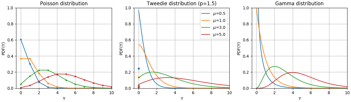](https://scikit-learn.org/stable/_images/poisson_gamma_tweedie_distributions.png)
PDF of a random variable Y following Poisson, Tweedie (power=1.5) and Gamma distributions with different mean values ( μ ). Observe the point mass at Y \= 0 for the Poisson distribution and the Tweedie (power=1.5) distribution, but not for the Gamma distribution which has a strictly positive target domain.[\#](https://scikit-learn.org/stable/modules/linear_model.html#id49 "Link to this image")
The Bernoulli distribution is a discrete probability distribution modelling a Bernoulli trial - an event that has only two mutually exclusive outcomes. The Categorical distribution is a generalization of the Bernoulli distribution for a categorical random variable. While a random variable in a Bernoulli distribution has two possible outcomes, a Categorical random variable can take on one of K possible categories, with the probability of each category specified separately.
The choice of the distribution depends on the problem at hand:
- If the target values y are counts (non-negative integer valued) or relative frequencies (non-negative), you might use a Poisson distribution with a log-link.
- If the target values are positive valued and skewed, you might try a Gamma distribution with a log-link.
- If the target values seem to be heavier tailed than a Gamma distribution, you might try an Inverse Gaussian distribution (or even higher variance powers of the Tweedie family).
- If the target values y are probabilities, you can use the Bernoulli distribution. The Bernoulli distribution with a logit link can be used for binary classification. The Categorical distribution with a softmax link can be used for multiclass classification.
Examples of use cases[\#](https://scikit-learn.org/stable/modules/linear_model.html#examples-of-use-cases "Link to this dropdown")
- Agriculture / weather modeling: number of rain events per year (Poisson), amount of rainfall per event (Gamma), total rainfall per year (Tweedie / Compound Poisson Gamma).
- Risk modeling / insurance policy pricing: number of claim events / policyholder per year (Poisson), cost per event (Gamma), total cost per policyholder per year (Tweedie / Compound Poisson Gamma).
- Credit Default: probability that a loan can’t be paid back (Bernoulli).
- Fraud Detection: probability that a financial transaction like a cash transfer is a fraudulent transaction (Bernoulli).
- Predictive maintenance: number of production interruption events per year (Poisson), duration of interruption (Gamma), total interruption time per year (Tweedie / Compound Poisson Gamma).
- Medical Drug Testing: probability of curing a patient in a set of trials or probability that a patient will experience side effects (Bernoulli).
- News Classification: classification of news articles into three categories namely Business News, Politics and Entertainment news (Categorical).
References
\[[10](https://scikit-learn.org/stable/modules/linear_model.html#id40)\]
McCullagh, Peter; Nelder, John (1989). Generalized Linear Models, Second Edition. Boca Raton: Chapman and Hall/CRC. ISBN 0-412-31760-5.
\[[11](https://scikit-learn.org/stable/modules/linear_model.html#id41)\]
Jørgensen, B. (1992). The theory of exponential dispersion models and analysis of deviance. Monografias de matemática, no. 51. See also [Exponential dispersion model.](https://en.wikipedia.org/wiki/Exponential_dispersion_model)
### 1\.1.12.1. Usage[\#](https://scikit-learn.org/stable/modules/linear_model.html#usage "Link to this heading")
[`TweedieRegressor`](https://scikit-learn.org/stable/modules/generated/sklearn.linear_model.TweedieRegressor.html#sklearn.linear_model.TweedieRegressor "sklearn.linear_model.TweedieRegressor") implements a generalized linear model for the Tweedie distribution, that allows to model any of the above mentioned distributions using the appropriate `power` parameter. In particular:
- `power = 0`: Normal distribution. Specific estimators such as [`Ridge`](https://scikit-learn.org/stable/modules/generated/sklearn.linear_model.Ridge.html#sklearn.linear_model.Ridge "sklearn.linear_model.Ridge"), [`ElasticNet`](https://scikit-learn.org/stable/modules/generated/sklearn.linear_model.ElasticNet.html#sklearn.linear_model.ElasticNet "sklearn.linear_model.ElasticNet") are generally more appropriate in this case.
- `power = 1`: Poisson distribution. [`PoissonRegressor`](https://scikit-learn.org/stable/modules/generated/sklearn.linear_model.PoissonRegressor.html#sklearn.linear_model.PoissonRegressor "sklearn.linear_model.PoissonRegressor") is exposed for convenience. However, it is strictly equivalent to `TweedieRegressor(power=1, link='log')`.
- `power = 2`: Gamma distribution. [`GammaRegressor`](https://scikit-learn.org/stable/modules/generated/sklearn.linear_model.GammaRegressor.html#sklearn.linear_model.GammaRegressor "sklearn.linear_model.GammaRegressor") is exposed for convenience. However, it is strictly equivalent to `TweedieRegressor(power=2, link='log')`.
- `power = 3`: Inverse Gaussian distribution.
The link function is determined by the `link` parameter.
Usage example:
```
>>> from sklearn.linear_model import TweedieRegressor
>>> reg = TweedieRegressor(power=1, alpha=0.5, link='log')
>>> reg.fit([[0, 0], [0, 1], [2, 2]], [0, 1, 2])
TweedieRegressor(alpha=0.5, link='log', power=1)
>>> reg.coef_
array([0.2463, 0.4337])
>>> reg.intercept_
np.float64(-0.7638)
```
Examples
- [Poisson regression and non-normal loss](https://scikit-learn.org/stable/auto_examples/linear_model/plot_poisson_regression_non_normal_loss.html#sphx-glr-auto-examples-linear-model-plot-poisson-regression-non-normal-loss-py)
- [Tweedie regression on insurance claims](https://scikit-learn.org/stable/auto_examples/linear_model/plot_tweedie_regression_insurance_claims.html#sphx-glr-auto-examples-linear-model-plot-tweedie-regression-insurance-claims-py)
Practical considerations[\#](https://scikit-learn.org/stable/modules/linear_model.html#practical-considerations "Link to this dropdown")
The feature matrix `X` should be standardized before fitting. This ensures that the penalty treats features equally.
Since the linear predictor X w can be negative and Poisson, Gamma and Inverse Gaussian distributions don’t support negative values, it is necessary to apply an inverse link function that guarantees the non-negativeness. For example with `link='log'`, the inverse link function becomes h ( X w ) \= exp ( X w ).
If you want to model a relative frequency, i.e. counts per exposure (time, volume, …) you can do so by using a Poisson distribution and passing y \= counts exposure as target values together with exposure as sample weights. For a concrete example see e.g. [Tweedie regression on insurance claims](https://scikit-learn.org/stable/auto_examples/linear_model/plot_tweedie_regression_insurance_claims.html#sphx-glr-auto-examples-linear-model-plot-tweedie-regression-insurance-claims-py).
When performing cross-validation for the `power` parameter of `TweedieRegressor`, it is advisable to specify an explicit `scoring` function, because the default scorer [`TweedieRegressor.score`](https://scikit-learn.org/stable/modules/generated/sklearn.linear_model.TweedieRegressor.html#sklearn.linear_model.TweedieRegressor.score "sklearn.linear_model.TweedieRegressor.score") is a function of `power` itself.
## 1\.1.13. Stochastic Gradient Descent - SGD[\#](https://scikit-learn.org/stable/modules/linear_model.html#stochastic-gradient-descent-sgd "Link to this heading")
Stochastic gradient descent is a simple yet very efficient approach to fit linear models. It is particularly useful when the number of samples (and the number of features) is very large. The `partial_fit` method allows online/out-of-core learning.
The classes [`SGDClassifier`](https://scikit-learn.org/stable/modules/generated/sklearn.linear_model.SGDClassifier.html#sklearn.linear_model.SGDClassifier "sklearn.linear_model.SGDClassifier") and [`SGDRegressor`](https://scikit-learn.org/stable/modules/generated/sklearn.linear_model.SGDRegressor.html#sklearn.linear_model.SGDRegressor "sklearn.linear_model.SGDRegressor") provide functionality to fit linear models for classification and regression using different (convex) loss functions and different penalties. E.g., with `loss="log"`, [`SGDClassifier`](https://scikit-learn.org/stable/modules/generated/sklearn.linear_model.SGDClassifier.html#sklearn.linear_model.SGDClassifier "sklearn.linear_model.SGDClassifier") fits a logistic regression model, while with `loss="hinge"` it fits a linear support vector machine (SVM).
You can refer to the dedicated [Stochastic Gradient Descent](https://scikit-learn.org/stable/modules/sgd.html#sgd) documentation section for more details.
### 1\.1.13.1. Perceptron[\#](https://scikit-learn.org/stable/modules/linear_model.html#perceptron "Link to this heading")
The [`Perceptron`](https://scikit-learn.org/stable/modules/generated/sklearn.linear_model.Perceptron.html#sklearn.linear_model.Perceptron "sklearn.linear_model.Perceptron") is another simple classification algorithm suitable for large scale learning and derives from SGD. By default:
- It does not require a learning rate.
- It is not regularized (penalized).
- It updates its model only on mistakes.
The last characteristic implies that the Perceptron is slightly faster to train than SGD with the hinge loss and that the resulting models are sparser.
In fact, the [`Perceptron`](https://scikit-learn.org/stable/modules/generated/sklearn.linear_model.Perceptron.html#sklearn.linear_model.Perceptron "sklearn.linear_model.Perceptron") is a wrapper around the [`SGDClassifier`](https://scikit-learn.org/stable/modules/generated/sklearn.linear_model.SGDClassifier.html#sklearn.linear_model.SGDClassifier "sklearn.linear_model.SGDClassifier") class using a perceptron loss and a constant learning rate. Refer to [mathematical section](https://scikit-learn.org/stable/modules/sgd.html#sgd-mathematical-formulation) of the SGD procedure for more details.
### 1\.1.13.2. Passive Aggressive Algorithms[\#](https://scikit-learn.org/stable/modules/linear_model.html#passive-aggressive-algorithms "Link to this heading")
The passive-aggressive (PA) algorithms are another family of 2 algorithms (PA-I and PA-II) for large-scale online learning that derive from SGD. They are similar to the Perceptron in that they do not require a learning rate. However, contrary to the Perceptron, they include a regularization parameter `eta0` (C in the reference paper).
For classification, `SGDClassifier(loss="hinge", penalty=None, learning_rate="pa1", eta0=1.0)` can be used for PA-I or with `learning_rate="pa2"` for PA-II. For regression, can be used for PA-I or with `learning_rate="pa2"` for PA-II.
References[\#](https://scikit-learn.org/stable/modules/linear_model.html#references-8 "Link to this dropdown")
- [“Online Passive-Aggressive Algorithms”](http://jmlr.csail.mit.edu/papers/volume7/crammer06a/crammer06a.pdf) K. Crammer, O. Dekel, J. Keshat, S. Shalev-Shwartz, Y. Singer - JMLR 7 (2006)
## 1\.1.14. Robustness regression: outliers and modeling errors[\#](https://scikit-learn.org/stable/modules/linear_model.html#robustness-regression-outliers-and-modeling-errors "Link to this heading")
Robust regression aims to fit a regression model in the presence of corrupt data: either outliers, or error in the model.
[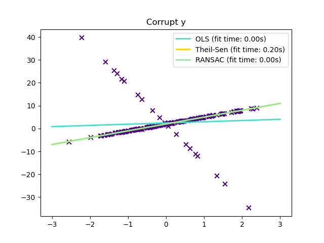](https://scikit-learn.org/stable/auto_examples/linear_model/plot_theilsen.html)
### 1\.1.14.1. Different scenario and useful concepts[\#](https://scikit-learn.org/stable/modules/linear_model.html#different-scenario-and-useful-concepts "Link to this heading")
There are different things to keep in mind when dealing with data corrupted by outliers:
- **Outliers in X or in y**?
| Outliers in the y direction | Outliers in the X direction |
|---|---|
| [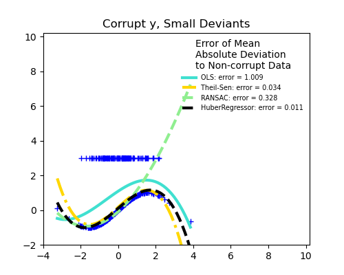](https://scikit-learn.org/stable/auto_examples/linear_model/plot_robust_fit.html) | [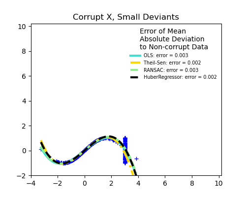](https://scikit-learn.org/stable/auto_examples/linear_model/plot_robust_fit.html) |
- **Fraction of outliers versus amplitude of error**
The number of outlying points matters, but also how much they are outliers.
| Small outliers | Large outliers |
|---|---|
| [](https://scikit-learn.org/stable/auto_examples/linear_model/plot_robust_fit.html) | [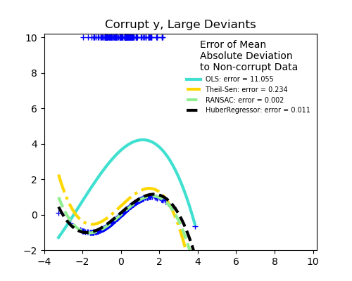](https://scikit-learn.org/stable/auto_examples/linear_model/plot_robust_fit.html) |
An important notion of robust fitting is that of breakdown point: the fraction of data that can be outlying for the fit to start missing the inlying data.
Note that in general, robust fitting in high-dimensional setting (large `n_features`) is very hard. The robust models here will probably not work in these settings.
Trade-offs: which estimator ?
Scikit-learn provides 3 robust regression estimators: [RANSAC](https://scikit-learn.org/stable/modules/linear_model.html#ransac-regression), [Theil Sen](https://scikit-learn.org/stable/modules/linear_model.html#theil-sen-regression) and [HuberRegressor](https://scikit-learn.org/stable/modules/linear_model.html#huber-regression).
- [HuberRegressor](https://scikit-learn.org/stable/modules/linear_model.html#huber-regression) should be faster than [RANSAC](https://scikit-learn.org/stable/modules/linear_model.html#ransac-regression) and [Theil Sen](https://scikit-learn.org/stable/modules/linear_model.html#theil-sen-regression) unless the number of samples is very large, i.e. `n_samples` \>\> `n_features`. This is because [RANSAC](https://scikit-learn.org/stable/modules/linear_model.html#ransac-regression) and [Theil Sen](https://scikit-learn.org/stable/modules/linear_model.html#theil-sen-regression) fit on smaller subsets of the data. However, both [Theil Sen](https://scikit-learn.org/stable/modules/linear_model.html#theil-sen-regression) and [RANSAC](https://scikit-learn.org/stable/modules/linear_model.html#ransac-regression) are unlikely to be as robust as [HuberRegressor](https://scikit-learn.org/stable/modules/linear_model.html#huber-regression) for the default parameters.
- [RANSAC](https://scikit-learn.org/stable/modules/linear_model.html#ransac-regression) is faster than [Theil Sen](https://scikit-learn.org/stable/modules/linear_model.html#theil-sen-regression) and scales much better with the number of samples.
- [RANSAC](https://scikit-learn.org/stable/modules/linear_model.html#ransac-regression) will deal better with large outliers in the y direction (most common situation).
- [Theil Sen](https://scikit-learn.org/stable/modules/linear_model.html#theil-sen-regression) will cope better with medium-size outliers in the X direction, but this property will disappear in high-dimensional settings.
When in doubt, use [RANSAC](https://scikit-learn.org/stable/modules/linear_model.html#ransac-regression).
### 1\.1.14.2. RANSAC: RANdom SAmple Consensus[\#](https://scikit-learn.org/stable/modules/linear_model.html#ransac-random-sample-consensus "Link to this heading")
RANSAC (RANdom SAmple Consensus) fits a model from random subsets of inliers from the complete data set.
RANSAC is a non-deterministic algorithm producing only a reasonable result with a certain probability, which is dependent on the number of iterations (see `max_trials` parameter). It is typically used for linear and non-linear regression problems and is especially popular in the field of photogrammetric computer vision.
The algorithm splits the complete input sample data into a set of inliers, which may be subject to noise, and outliers, which are e.g. caused by erroneous measurements or invalid hypotheses about the data. The resulting model is then estimated only from the determined inliers.
[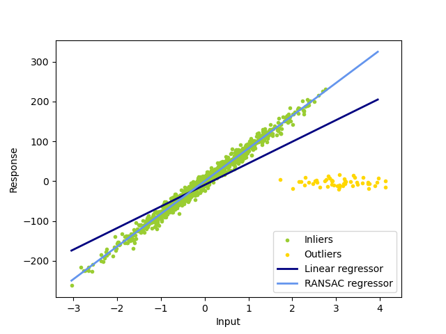](https://scikit-learn.org/stable/auto_examples/linear_model/plot_ransac.html)
Examples
- [Robust linear model estimation using RANSAC](https://scikit-learn.org/stable/auto_examples/linear_model/plot_ransac.html#sphx-glr-auto-examples-linear-model-plot-ransac-py)
- [Robust linear estimator fitting](https://scikit-learn.org/stable/auto_examples/linear_model/plot_robust_fit.html#sphx-glr-auto-examples-linear-model-plot-robust-fit-py)
Details of the algorithm[\#](https://scikit-learn.org/stable/modules/linear_model.html#details-of-the-algorithm "Link to this dropdown")
Each iteration performs the following steps:
1. Select `min_samples` random samples from the original data and check whether the set of data is valid (see `is_data_valid`).
2. Fit a model to the random subset (`estimator.fit`) and check whether the estimated model is valid (see `is_model_valid`).
3. Classify all data as inliers or outliers by calculating the residuals to the estimated model (`estimator.predict(X) - y`) - all data samples with absolute residuals smaller than or equal to the `residual_threshold` are considered as inliers.
4. Save fitted model as best model if number of inlier samples is maximal. In case the current estimated model has the same number of inliers, it is only considered as the best model if it has better score.
These steps are performed either a maximum number of times (`max_trials`) or until one of the special stop criteria are met (see `stop_n_inliers` and `stop_score`). The final model is estimated using all inlier samples (consensus set) of the previously determined best model.
The `is_data_valid` and `is_model_valid` functions allow to identify and reject degenerate combinations of random sub-samples. If the estimated model is not needed for identifying degenerate cases, `is_data_valid` should be used as it is called prior to fitting the model and thus leading to better computational performance.
References[\#](https://scikit-learn.org/stable/modules/linear_model.html#references-9 "Link to this dropdown")
- <https://en.wikipedia.org/wiki/RANSAC>
- [“Random Sample Consensus: A Paradigm for Model Fitting with Applications to Image Analysis and Automated Cartography”](https://www.cs.ait.ac.th/~mdailey/cvreadings/Fischler-RANSAC.pdf) Martin A. Fischler and Robert C. Bolles - SRI International (1981)
- [“Performance Evaluation of RANSAC Family”](http://www.bmva.org/bmvc/2009/Papers/Paper355/Paper355.pdf) Sunglok Choi, Taemin Kim and Wonpil Yu - BMVC (2009)
### 1\.1.14.3. Theil-Sen estimator: generalized-median-based estimator[\#](https://scikit-learn.org/stable/modules/linear_model.html#theil-sen-estimator-generalized-median-based-estimator "Link to this heading")
The [`TheilSenRegressor`](https://scikit-learn.org/stable/modules/generated/sklearn.linear_model.TheilSenRegressor.html#sklearn.linear_model.TheilSenRegressor "sklearn.linear_model.TheilSenRegressor") estimator uses a generalization of the median in multiple dimensions. It is thus robust to multivariate outliers. Note however that the robustness of the estimator decreases quickly with the dimensionality of the problem. It loses its robustness properties and becomes no better than an ordinary least squares in high dimension.
Examples
- [Theil-Sen Regression](https://scikit-learn.org/stable/auto_examples/linear_model/plot_theilsen.html#sphx-glr-auto-examples-linear-model-plot-theilsen-py)
- [Robust linear estimator fitting](https://scikit-learn.org/stable/auto_examples/linear_model/plot_robust_fit.html#sphx-glr-auto-examples-linear-model-plot-robust-fit-py)
Theoretical considerations[\#](https://scikit-learn.org/stable/modules/linear_model.html#theoretical-considerations "Link to this dropdown")
[`TheilSenRegressor`](https://scikit-learn.org/stable/modules/generated/sklearn.linear_model.TheilSenRegressor.html#sklearn.linear_model.TheilSenRegressor "sklearn.linear_model.TheilSenRegressor") is comparable to the [Ordinary Least Squares (OLS)](https://scikit-learn.org/stable/modules/linear_model.html#ordinary-least-squares) in terms of asymptotic efficiency and as an unbiased estimator. In contrast to OLS, Theil-Sen is a non-parametric method which means it makes no assumption about the underlying distribution of the data. Since Theil-Sen is a median-based estimator, it is more robust against corrupted data aka outliers. In univariate setting, Theil-Sen has a breakdown point of about 29.3% in case of a simple linear regression which means that it can tolerate arbitrary corrupted data of up to 29.3%.
[](https://scikit-learn.org/stable/auto_examples/linear_model/plot_theilsen.html)
The implementation of [`TheilSenRegressor`](https://scikit-learn.org/stable/modules/generated/sklearn.linear_model.TheilSenRegressor.html#sklearn.linear_model.TheilSenRegressor "sklearn.linear_model.TheilSenRegressor") in scikit-learn follows a generalization to a multivariate linear regression model [\[14\]](https://scikit-learn.org/stable/modules/linear_model.html#f1) using the spatial median which is a generalization of the median to multiple dimensions [\[15\]](https://scikit-learn.org/stable/modules/linear_model.html#f2).
In terms of time and space complexity, Theil-Sen scales according to
(
n
samples
n
subsamples
)
which makes it infeasible to be applied exhaustively to problems with a large number of samples and features. Therefore, the magnitude of a subpopulation can be chosen to limit the time and space complexity by considering only a random subset of all possible combinations.
References
\[[14](https://scikit-learn.org/stable/modules/linear_model.html#id45)\]
Xin Dang, Hanxiang Peng, Xueqin Wang and Heping Zhang: [Theil-Sen Estimators in a Multiple Linear Regression Model.](http://home.olemiss.edu/~xdang/papers/MTSE.pdf)
\[[15](https://scikit-learn.org/stable/modules/linear_model.html#id46)\]
1. Kärkkäinen and S. Äyrämö: [On Computation of Spatial Median for Robust Data Mining.](http://users.jyu.fi/~samiayr/pdf/ayramo_eurogen05.pdf)
Also see the [Wikipedia page](https://en.wikipedia.org/wiki/Theil%E2%80%93Sen_estimator)
### 1\.1.14.4. Huber Regression[\#](https://scikit-learn.org/stable/modules/linear_model.html#huber-regression "Link to this heading")
The [`HuberRegressor`](https://scikit-learn.org/stable/modules/generated/sklearn.linear_model.HuberRegressor.html#sklearn.linear_model.HuberRegressor "sklearn.linear_model.HuberRegressor") is different from [`Ridge`](https://scikit-learn.org/stable/modules/generated/sklearn.linear_model.Ridge.html#sklearn.linear_model.Ridge "sklearn.linear_model.Ridge") because it applies a linear loss to samples that are defined as outliers by the `epsilon` parameter. A sample is classified as an inlier if the absolute error of that sample is less than the threshold `epsilon`. It differs from [`TheilSenRegressor`](https://scikit-learn.org/stable/modules/generated/sklearn.linear_model.TheilSenRegressor.html#sklearn.linear_model.TheilSenRegressor "sklearn.linear_model.TheilSenRegressor") and [`RANSACRegressor`](https://scikit-learn.org/stable/modules/generated/sklearn.linear_model.RANSACRegressor.html#sklearn.linear_model.RANSACRegressor "sklearn.linear_model.RANSACRegressor") because it does not ignore the effect of the outliers but gives a lesser weight to them.
[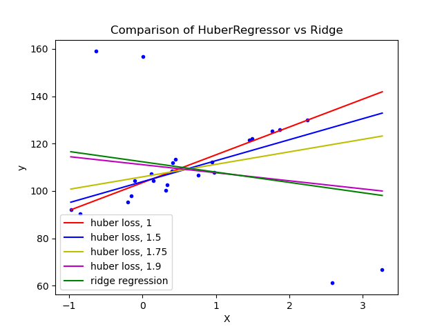](https://scikit-learn.org/stable/auto_examples/linear_model/plot_huber_vs_ridge.html)
Examples
- [HuberRegressor vs Ridge on dataset with strong outliers](https://scikit-learn.org/stable/auto_examples/linear_model/plot_huber_vs_ridge.html#sphx-glr-auto-examples-linear-model-plot-huber-vs-ridge-py)
Mathematical details[\#](https://scikit-learn.org/stable/modules/linear_model.html#mathematical-details-5 "Link to this dropdown")
[`HuberRegressor`](https://scikit-learn.org/stable/modules/generated/sklearn.linear_model.HuberRegressor.html#sklearn.linear_model.HuberRegressor "sklearn.linear_model.HuberRegressor") minimizes
min
w
,
σ
∑
i
\=
1
n
(
σ
\+
H
ϵ
(
X
i
w
−
y
i
σ
)
σ
)
\+
α
\|
\|
w
\|
\|
2
2
where the loss function is given by
H
ϵ
(
z
)
\=
{
z
2
,
if
\|
z
\|
\<
ϵ
,
2
ϵ
\|
z
\|
−
ϵ
2
,
otherwise
It is advised to set the parameter `epsilon` to 1.35 to achieve 95% statistical efficiency.
References
- Peter J. Huber, Elvezio M. Ronchetti: Robust Statistics, Concomitant scale estimates, p. 172.
The [`HuberRegressor`](https://scikit-learn.org/stable/modules/generated/sklearn.linear_model.HuberRegressor.html#sklearn.linear_model.HuberRegressor "sklearn.linear_model.HuberRegressor") differs from using [`SGDRegressor`](https://scikit-learn.org/stable/modules/generated/sklearn.linear_model.SGDRegressor.html#sklearn.linear_model.SGDRegressor "sklearn.linear_model.SGDRegressor") with loss set to `huber` in the following ways.
- [`HuberRegressor`](https://scikit-learn.org/stable/modules/generated/sklearn.linear_model.HuberRegressor.html#sklearn.linear_model.HuberRegressor "sklearn.linear_model.HuberRegressor") is scaling invariant. Once `epsilon` is set, scaling `X` and `y` down or up by different values would produce the same robustness to outliers as before. as compared to [`SGDRegressor`](https://scikit-learn.org/stable/modules/generated/sklearn.linear_model.SGDRegressor.html#sklearn.linear_model.SGDRegressor "sklearn.linear_model.SGDRegressor") where `epsilon` has to be set again when `X` and `y` are scaled.
- [`HuberRegressor`](https://scikit-learn.org/stable/modules/generated/sklearn.linear_model.HuberRegressor.html#sklearn.linear_model.HuberRegressor "sklearn.linear_model.HuberRegressor") should be more efficient to use on data with small number of samples while [`SGDRegressor`](https://scikit-learn.org/stable/modules/generated/sklearn.linear_model.SGDRegressor.html#sklearn.linear_model.SGDRegressor "sklearn.linear_model.SGDRegressor") needs a number of passes on the training data to produce the same robustness.
Note that this estimator is different from the [R implementation of Robust Regression](https://stats.oarc.ucla.edu/r/dae/robust-regression/) because the R implementation does a weighted least squares implementation with weights given to each sample on the basis of how much the residual is greater than a certain threshold.
## 1\.1.15. Quantile Regression[\#](https://scikit-learn.org/stable/modules/linear_model.html#quantile-regression "Link to this heading")
Quantile regression estimates the median or other quantiles of y conditional on X, while ordinary least squares (OLS) estimates the conditional mean.
Quantile regression may be useful if one is interested in predicting an interval instead of point prediction. Sometimes, prediction intervals are calculated based on the assumption that prediction error is distributed normally with zero mean and constant variance. Quantile regression provides sensible prediction intervals even for errors with non-constant (but predictable) variance or non-normal distribution.
[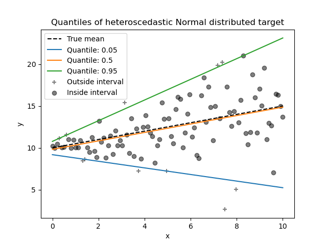](https://scikit-learn.org/stable/auto_examples/linear_model/plot_quantile_regression.html)
Based on minimizing the pinball loss, conditional quantiles can also be estimated by models other than linear models. For example, [`GradientBoostingRegressor`](https://scikit-learn.org/stable/modules/generated/sklearn.ensemble.GradientBoostingRegressor.html#sklearn.ensemble.GradientBoostingRegressor "sklearn.ensemble.GradientBoostingRegressor") can predict conditional quantiles if its parameter `loss` is set to `"quantile"` and parameter `alpha` is set to the quantile that should be predicted. See the example in [Prediction Intervals for Gradient Boosting Regression](https://scikit-learn.org/stable/auto_examples/ensemble/plot_gradient_boosting_quantile.html#sphx-glr-auto-examples-ensemble-plot-gradient-boosting-quantile-py).
Most implementations of quantile regression are based on linear programming problem. The current implementation is based on [`scipy.optimize.linprog`](https://docs.scipy.org/doc/scipy/reference/generated/scipy.optimize.linprog.html#scipy.optimize.linprog "(in SciPy v1.17.0)").
Examples
- [Quantile regression](https://scikit-learn.org/stable/auto_examples/linear_model/plot_quantile_regression.html#sphx-glr-auto-examples-linear-model-plot-quantile-regression-py)
Mathematical details[\#](https://scikit-learn.org/stable/modules/linear_model.html#mathematical-details-6 "Link to this dropdown")
As a linear model, the [`QuantileRegressor`](https://scikit-learn.org/stable/modules/generated/sklearn.linear_model.QuantileRegressor.html#sklearn.linear_model.QuantileRegressor "sklearn.linear_model.QuantileRegressor") gives linear predictions y ^ ( w , X ) \= X w for the q\-th quantile, q ∈ ( 0 , 1 ). The weights or coefficients w are then found by the following minimization problem:
min
w
1
n
samples
∑
i
P
B
q
(
y
i
−
X
i
w
)
\+
α
\|
\|
w
\|
\|
1
.
This consists of the pinball loss (also known as linear loss), see also [`mean_pinball_loss`](https://scikit-learn.org/stable/modules/generated/sklearn.metrics.mean_pinball_loss.html#sklearn.metrics.mean_pinball_loss "sklearn.metrics.mean_pinball_loss"),
P
B
q
(
t
)
\=
q
max
(
t
,
0
)
\+
(
1
−
q
)
max
(
−
t
,
0
)
\=
{
q
t
,
t
\>
0
,
0
,
t
\=
0
,
(
q
−
1
)
t
,
t
\<
0
and the L1 penalty controlled by parameter `alpha`, similar to [`Lasso`](https://scikit-learn.org/stable/modules/generated/sklearn.linear_model.Lasso.html#sklearn.linear_model.Lasso "sklearn.linear_model.Lasso").
As the pinball loss is only linear in the residuals, quantile regression is much more robust to outliers than squared error based estimation of the mean. Somewhat in between is the [`HuberRegressor`](https://scikit-learn.org/stable/modules/generated/sklearn.linear_model.HuberRegressor.html#sklearn.linear_model.HuberRegressor "sklearn.linear_model.HuberRegressor").
References[\#](https://scikit-learn.org/stable/modules/linear_model.html#references-10 "Link to this dropdown")
- Koenker, R., & Bassett Jr, G. (1978). [Regression quantiles.](https://gib.people.uic.edu/RQ.pdf) Econometrica: journal of the Econometric Society, 33-50.
- Portnoy, S., & Koenker, R. (1997). [The Gaussian hare and the Laplacian tortoise: computability of squared-error versus absolute-error estimators. Statistical Science, 12, 279-300](https://doi.org/10.1214/ss/1030037960).
- Koenker, R. (2005). [Quantile Regression](https://doi.org/10.1017/CBO9780511754098). Cambridge University Press.
## 1\.1.16. Polynomial regression: extending linear models with basis functions[\#](https://scikit-learn.org/stable/modules/linear_model.html#polynomial-regression-extending-linear-models-with-basis-functions "Link to this heading")
One common pattern within machine learning is to use linear models trained on nonlinear functions of the data. This approach maintains the generally fast performance of linear methods, while allowing them to fit a much wider range of data.
Mathematical details[\#](https://scikit-learn.org/stable/modules/linear_model.html#mathematical-details-7 "Link to this dropdown")
For example, a simple linear regression can be extended by constructing **polynomial features** from the coefficients. In the standard linear regression case, you might have a model that looks like this for two-dimensional data:
y
^
(
w
,
x
)
\=
w
0
\+
w
1
x
1
\+
w
2
x
2
If we want to fit a paraboloid to the data instead of a plane, we can combine the features in second-order polynomials, so that the model looks like this:
y
^
(
w
,
x
)
\=
w
0
\+
w
1
x
1
\+
w
2
x
2
\+
w
3
x
1
x
2
\+
w
4
x
1
2
\+
w
5
x
2
2
The (sometimes surprising) observation is that this is *still a linear model*: to see this, imagine creating a new set of features
z
\=
\[
x
1
,
x
2
,
x
1
x
2
,
x
1
2
,
x
2
2
\]
With this re-labeling of the data, our problem can be written
y
^
(
w
,
z
)
\=
w
0
\+
w
1
z
1
\+
w
2
z
2
\+
w
3
z
3
\+
w
4
z
4
\+
w
5
z
5
We see that the resulting *polynomial regression* is in the same class of linear models we considered above (i.e. the model is linear in w) and can be solved by the same techniques. By considering linear fits within a higher-dimensional space built with these basis functions, the model has the flexibility to fit a much broader range of data.
Here is an example of applying this idea to one-dimensional data, using polynomial features of varying degrees:
[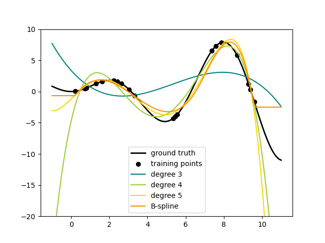](https://scikit-learn.org/stable/auto_examples/linear_model/plot_polynomial_interpolation.html)
This figure is created using the [`PolynomialFeatures`](https://scikit-learn.org/stable/modules/generated/sklearn.preprocessing.PolynomialFeatures.html#sklearn.preprocessing.PolynomialFeatures "sklearn.preprocessing.PolynomialFeatures") transformer, which transforms an input data matrix into a new data matrix of a given degree. It can be used as follows:
```
>>> from sklearn.preprocessing import PolynomialFeatures
>>> import numpy as np
>>> X = np.arange(6).reshape(3, 2)
>>> X
array([[0, 1],
[2, 3],
[4, 5]])
>>> poly = PolynomialFeatures(degree=2)
>>> poly.fit_transform(X)
array([[ 1., 0., 1., 0., 0., 1.],
[ 1., 2., 3., 4., 6., 9.],
[ 1., 4., 5., 16., 20., 25.]])
```
The features of `X` have been transformed from \[ x 1 , x 2 \] to \[ 1 , x 1 , x 2 , x 1 2 , x 1 x 2 , x 2 2 \], and can now be used within any linear model.
This sort of preprocessing can be streamlined with the [Pipeline](https://scikit-learn.org/stable/modules/compose.html#pipeline) tools. A single object representing a simple polynomial regression can be created and used as follows:
```
>>> from sklearn.preprocessing import PolynomialFeatures
>>> from sklearn.linear_model import LinearRegression
>>> from sklearn.pipeline import Pipeline
>>> import numpy as np
>>> model = Pipeline([('poly', PolynomialFeatures(degree=3)),
... ('linear', LinearRegression(fit_intercept=False))])
>>> # fit to an order-3 polynomial data
>>> x = np.arange(5)
>>> y = 3 - 2 * x + x ** 2 - x ** 3
>>> model = model.fit(x[:, np.newaxis], y)
>>> model.named_steps['linear'].coef_
array([ 3., -2., 1., -1.])
```
The linear model trained on polynomial features is able to exactly recover the input polynomial coefficients.
In some cases it’s not necessary to include higher powers of any single feature, but only the so-called *interaction features* that multiply together at most d distinct features. These can be gotten from [`PolynomialFeatures`](https://scikit-learn.org/stable/modules/generated/sklearn.preprocessing.PolynomialFeatures.html#sklearn.preprocessing.PolynomialFeatures "sklearn.preprocessing.PolynomialFeatures") with the setting `interaction_only=True`.
For example, when dealing with boolean features, x i n \= x i for all n and is therefore useless; but x i x j represents the conjunction of two booleans. This way, we can solve the XOR problem with a linear classifier:
```
>>> from sklearn.linear_model import Perceptron
>>> from sklearn.preprocessing import PolynomialFeatures
>>> import numpy as np
>>> X = np.array([[0, 0], [0, 1], [1, 0], [1, 1]])
>>> y = X[:, 0] ^ X[:, 1]
>>> y
array([0, 1, 1, 0])
>>> X = PolynomialFeatures(interaction_only=True).fit_transform(X).astype(int)
>>> X
array([[1, 0, 0, 0],
[1, 0, 1, 0],
[1, 1, 0, 0],
[1, 1, 1, 1]])
>>> clf = Perceptron(fit_intercept=False, max_iter=10, tol=None,
... shuffle=False).fit(X, y)
```
And the classifier “predictions” are perfect:
```
>>> clf.predict(X)
array([0, 1, 1, 0])
>>> clf.score(X, y)
1.0
```
[previous 1. Supervised learning](https://scikit-learn.org/stable/supervised_learning.html "previous page")
[next 1.2. Linear and Quadratic Discriminant Analysis](https://scikit-learn.org/stable/modules/lda_qda.html "next page")
On this page
- [1\.1.1. Ordinary Least Squares](https://scikit-learn.org/stable/modules/linear_model.html#ordinary-least-squares)
- [1\.1.1.1. Non-Negative Least Squares](https://scikit-learn.org/stable/modules/linear_model.html#non-negative-least-squares)
- [1\.1.1.2. Ordinary Least Squares Complexity](https://scikit-learn.org/stable/modules/linear_model.html#ordinary-least-squares-complexity)
- [1\.1.2. Ridge regression and classification](https://scikit-learn.org/stable/modules/linear_model.html#ridge-regression-and-classification)
- [1\.1.2.1. Regression](https://scikit-learn.org/stable/modules/linear_model.html#regression)
- [1\.1.2.2. Classification](https://scikit-learn.org/stable/modules/linear_model.html#classification)
- [1\.1.2.3. Ridge Complexity](https://scikit-learn.org/stable/modules/linear_model.html#ridge-complexity)
- [1\.1.2.4. Setting the regularization parameter: leave-one-out Cross-Validation](https://scikit-learn.org/stable/modules/linear_model.html#setting-the-regularization-parameter-leave-one-out-cross-validation)
- [1\.1.3. Lasso](https://scikit-learn.org/stable/modules/linear_model.html#lasso)
- [1\.1.3.1. Coordinate Descent with Gap Safe Screening Rules](https://scikit-learn.org/stable/modules/linear_model.html#coordinate-descent-with-gap-safe-screening-rules)
- [1\.1.3.2. Setting regularization parameter](https://scikit-learn.org/stable/modules/linear_model.html#setting-regularization-parameter)
- [1\.1.3.2.1. Using cross-validation](https://scikit-learn.org/stable/modules/linear_model.html#using-cross-validation)
- [1\.1.3.2.2. Information-criteria based model selection](https://scikit-learn.org/stable/modules/linear_model.html#information-criteria-based-model-selection)
- [1\.1.3.2.3. AIC and BIC criteria](https://scikit-learn.org/stable/modules/linear_model.html#aic-and-bic-criteria)
- [1\.1.3.2.4. Comparison with the regularization parameter of SVM](https://scikit-learn.org/stable/modules/linear_model.html#comparison-with-the-regularization-parameter-of-svm)
- [1\.1.4. Multi-task Lasso](https://scikit-learn.org/stable/modules/linear_model.html#multi-task-lasso)
- [1\.1.5. Elastic-Net](https://scikit-learn.org/stable/modules/linear_model.html#elastic-net)
- [1\.1.6. Multi-task Elastic-Net](https://scikit-learn.org/stable/modules/linear_model.html#multi-task-elastic-net)
- [1\.1.7. Least Angle Regression](https://scikit-learn.org/stable/modules/linear_model.html#least-angle-regression)
- [1\.1.8. LARS Lasso](https://scikit-learn.org/stable/modules/linear_model.html#lars-lasso)
- [1\.1.9. Orthogonal Matching Pursuit (OMP)](https://scikit-learn.org/stable/modules/linear_model.html#orthogonal-matching-pursuit-omp)
- [1\.1.10. Bayesian Regression](https://scikit-learn.org/stable/modules/linear_model.html#bayesian-regression)
- [1\.1.10.1. Bayesian Ridge Regression](https://scikit-learn.org/stable/modules/linear_model.html#bayesian-ridge-regression)
- [1\.1.10.2. Automatic Relevance Determination - ARD](https://scikit-learn.org/stable/modules/linear_model.html#automatic-relevance-determination-ard)
- [1\.1.11. Logistic regression](https://scikit-learn.org/stable/modules/linear_model.html#logistic-regression)
- [1\.1.11.1. Binary Case](https://scikit-learn.org/stable/modules/linear_model.html#binary-case)
- [1\.1.11.2. Multinomial Case](https://scikit-learn.org/stable/modules/linear_model.html#multinomial-case)
- [1\.1.11.3. Solvers](https://scikit-learn.org/stable/modules/linear_model.html#solvers)
- [1\.1.11.3.1. Differences between solvers](https://scikit-learn.org/stable/modules/linear_model.html#differences-between-solvers)
- [1\.1.12. Generalized Linear Models](https://scikit-learn.org/stable/modules/linear_model.html#generalized-linear-models)
- [1\.1.12.1. Usage](https://scikit-learn.org/stable/modules/linear_model.html#usage)
- [1\.1.13. Stochastic Gradient Descent - SGD](https://scikit-learn.org/stable/modules/linear_model.html#stochastic-gradient-descent-sgd)
- [1\.1.13.1. Perceptron](https://scikit-learn.org/stable/modules/linear_model.html#perceptron)
- [1\.1.13.2. Passive Aggressive Algorithms](https://scikit-learn.org/stable/modules/linear_model.html#passive-aggressive-algorithms)
- [1\.1.14. Robustness regression: outliers and modeling errors](https://scikit-learn.org/stable/modules/linear_model.html#robustness-regression-outliers-and-modeling-errors)
- [1\.1.14.1. Different scenario and useful concepts](https://scikit-learn.org/stable/modules/linear_model.html#different-scenario-and-useful-concepts)
- [1\.1.14.2. RANSAC: RANdom SAmple Consensus](https://scikit-learn.org/stable/modules/linear_model.html#ransac-random-sample-consensus)
- [1\.1.14.3. Theil-Sen estimator: generalized-median-based estimator](https://scikit-learn.org/stable/modules/linear_model.html#theil-sen-estimator-generalized-median-based-estimator)
- [1\.1.14.4. Huber Regression](https://scikit-learn.org/stable/modules/linear_model.html#huber-regression)
- [1\.1.15. Quantile Regression](https://scikit-learn.org/stable/modules/linear_model.html#quantile-regression)
- [1\.1.16. Polynomial regression: extending linear models with basis functions](https://scikit-learn.org/stable/modules/linear_model.html#polynomial-regression-extending-linear-models-with-basis-functions)
### This Page
- [Show Source](https://scikit-learn.org/stable/_sources/modules/linear_model.rst.txt)
© Copyright 2007 - 2026, scikit-learn developers (BSD License). |
| Readable Markdown | The following are a set of methods intended for regression in which the target value is expected to be a linear combination of the features. In mathematical notation, if y ^ is the predicted value.
y ^ ( w , x ) \= w 0 \+ w 1 x 1 \+ . . . \+ w p x p
Across the module, we designate the vector w \= ( w 1 , . . . , w p ) as `coef_` and w 0 as `intercept_`.
To perform classification with generalized linear models, see [Logistic regression](https://scikit-learn.org/stable/modules/linear_model.html#logistic-regression).
## 1\.1.1. Ordinary Least Squares[\#](https://scikit-learn.org/stable/modules/linear_model.html#ordinary-least-squares "Link to this heading")
[`LinearRegression`](https://scikit-learn.org/stable/modules/generated/sklearn.linear_model.LinearRegression.html#sklearn.linear_model.LinearRegression "sklearn.linear_model.LinearRegression") fits a linear model with coefficients w \= ( w 1 , . . . , w p ) to minimize the residual sum of squares between the observed targets in the dataset, and the targets predicted by the linear approximation. Mathematically it solves a problem of the form:
min w \| \| X w − y \| \| 2 2
[](https://scikit-learn.org/stable/auto_examples/linear_model/plot_ols_ridge.html)
[`LinearRegression`](https://scikit-learn.org/stable/modules/generated/sklearn.linear_model.LinearRegression.html#sklearn.linear_model.LinearRegression "sklearn.linear_model.LinearRegression") takes in its `fit` method arguments `X`, `y`, `sample_weight` and stores the coefficients w of the linear model in its `coef_` and `intercept_` attributes:
```
>>> from sklearn import linear_model
>>> reg = linear_model.LinearRegression()
>>> reg.fit([[0, 0], [1, 1], [2, 2]], [0, 1, 2])
LinearRegression()
>>> reg.coef_
array([0.5, 0.5])
>>> reg.intercept_
0.0
```
The coefficient estimates for Ordinary Least Squares rely on the independence of the features. When features are correlated and some columns of the design matrix X have an approximately linear dependence, the design matrix becomes close to singular and as a result, the least-squares estimate becomes highly sensitive to random errors in the observed target, producing a large variance. This situation of *multicollinearity* can arise, for example, when data are collected without an experimental design.
Examples
- [Ordinary Least Squares and Ridge Regression](https://scikit-learn.org/stable/auto_examples/linear_model/plot_ols_ridge.html#sphx-glr-auto-examples-linear-model-plot-ols-ridge-py)
### 1\.1.1.1. Non-Negative Least Squares[\#](https://scikit-learn.org/stable/modules/linear_model.html#non-negative-least-squares "Link to this heading")
It is possible to constrain all the coefficients to be non-negative, which may be useful when they represent some physical or naturally non-negative quantities (e.g., frequency counts or prices of goods). [`LinearRegression`](https://scikit-learn.org/stable/modules/generated/sklearn.linear_model.LinearRegression.html#sklearn.linear_model.LinearRegression "sklearn.linear_model.LinearRegression") accepts a boolean `positive` parameter: when set to `True` [Non-Negative Least Squares](https://en.wikipedia.org/wiki/Non-negative_least_squares) are then applied.
Examples
- [Non-negative least squares](https://scikit-learn.org/stable/auto_examples/linear_model/plot_nnls.html#sphx-glr-auto-examples-linear-model-plot-nnls-py)
### 1\.1.1.2. Ordinary Least Squares Complexity[\#](https://scikit-learn.org/stable/modules/linear_model.html#ordinary-least-squares-complexity "Link to this heading")
The least squares solution is computed using the singular value decomposition of X. If X is a matrix of shape `(n_samples, n_features)` this method has a cost of O ( n samples n features 2 ), assuming that n samples ≥ n features.
## 1\.1.2. Ridge regression and classification[\#](https://scikit-learn.org/stable/modules/linear_model.html#ridge-regression-and-classification "Link to this heading")
### 1\.1.2.1. Regression[\#](https://scikit-learn.org/stable/modules/linear_model.html#regression "Link to this heading")
[`Ridge`](https://scikit-learn.org/stable/modules/generated/sklearn.linear_model.Ridge.html#sklearn.linear_model.Ridge "sklearn.linear_model.Ridge") regression addresses some of the problems of [Ordinary Least Squares](https://scikit-learn.org/stable/modules/linear_model.html#ordinary-least-squares) by imposing a penalty on the size of the coefficients. The ridge coefficients minimize a penalized residual sum of squares:
min w \| \| X w − y \| \| 2 2 \+ α \| \| w \| \| 2 2
The complexity parameter α ≥ 0 controls the amount of shrinkage: the larger the value of α, the greater the amount of shrinkage and thus the coefficients become more robust to collinearity.
[](https://scikit-learn.org/stable/auto_examples/linear_model/plot_ridge_path.html)
As with other linear models, [`Ridge`](https://scikit-learn.org/stable/modules/generated/sklearn.linear_model.Ridge.html#sklearn.linear_model.Ridge "sklearn.linear_model.Ridge") will take in its `fit` method arrays `X`, `y` and will store the coefficients w of the linear model in its `coef_` member:
```
>>> from sklearn import linear_model
>>> reg = linear_model.Ridge(alpha=.5)
>>> reg.fit([[0, 0], [0, 0], [1, 1]], [0, .1, 1])
Ridge(alpha=0.5)
>>> reg.coef_
array([0.34545455, 0.34545455])
>>> reg.intercept_
np.float64(0.13636)
```
Note that the class [`Ridge`](https://scikit-learn.org/stable/modules/generated/sklearn.linear_model.Ridge.html#sklearn.linear_model.Ridge "sklearn.linear_model.Ridge") allows for the user to specify that the solver be automatically chosen by setting `solver="auto"`. When this option is specified, [`Ridge`](https://scikit-learn.org/stable/modules/generated/sklearn.linear_model.Ridge.html#sklearn.linear_model.Ridge "sklearn.linear_model.Ridge") will choose between the `"lbfgs"`, `"cholesky"`, and `"sparse_cg"` solvers. [`Ridge`](https://scikit-learn.org/stable/modules/generated/sklearn.linear_model.Ridge.html#sklearn.linear_model.Ridge "sklearn.linear_model.Ridge") will begin checking the conditions shown in the following table from top to bottom. If the condition is true, the corresponding solver is chosen.
Examples
- [Ordinary Least Squares and Ridge Regression](https://scikit-learn.org/stable/auto_examples/linear_model/plot_ols_ridge.html#sphx-glr-auto-examples-linear-model-plot-ols-ridge-py)
- [Plot Ridge coefficients as a function of the regularization](https://scikit-learn.org/stable/auto_examples/linear_model/plot_ridge_path.html#sphx-glr-auto-examples-linear-model-plot-ridge-path-py)
- [Common pitfalls in the interpretation of coefficients of linear models](https://scikit-learn.org/stable/auto_examples/inspection/plot_linear_model_coefficient_interpretation.html#sphx-glr-auto-examples-inspection-plot-linear-model-coefficient-interpretation-py)
- [Ridge coefficients as a function of the L2 Regularization](https://scikit-learn.org/stable/auto_examples/linear_model/plot_ridge_coeffs.html#sphx-glr-auto-examples-linear-model-plot-ridge-coeffs-py)
### 1\.1.2.2. Classification[\#](https://scikit-learn.org/stable/modules/linear_model.html#classification "Link to this heading")
The [`Ridge`](https://scikit-learn.org/stable/modules/generated/sklearn.linear_model.Ridge.html#sklearn.linear_model.Ridge "sklearn.linear_model.Ridge") regressor has a classifier variant: [`RidgeClassifier`](https://scikit-learn.org/stable/modules/generated/sklearn.linear_model.RidgeClassifier.html#sklearn.linear_model.RidgeClassifier "sklearn.linear_model.RidgeClassifier"). This classifier first converts binary targets to `{-1, 1}` and then treats the problem as a regression task, optimizing the same objective as above. The predicted class corresponds to the sign of the regressor’s prediction. For multiclass classification, the problem is treated as multi-output regression, and the predicted class corresponds to the output with the highest value.
It might seem questionable to use a (penalized) Least Squares loss to fit a classification model instead of the more traditional logistic or hinge losses. However, in practice, all those models can lead to similar cross-validation scores in terms of accuracy or precision/recall, while the penalized least squares loss used by the [`RidgeClassifier`](https://scikit-learn.org/stable/modules/generated/sklearn.linear_model.RidgeClassifier.html#sklearn.linear_model.RidgeClassifier "sklearn.linear_model.RidgeClassifier") allows for a very different choice of the numerical solvers with distinct computational performance profiles.
The [`RidgeClassifier`](https://scikit-learn.org/stable/modules/generated/sklearn.linear_model.RidgeClassifier.html#sklearn.linear_model.RidgeClassifier "sklearn.linear_model.RidgeClassifier") can be significantly faster than e.g. [`LogisticRegression`](https://scikit-learn.org/stable/modules/generated/sklearn.linear_model.LogisticRegression.html#sklearn.linear_model.LogisticRegression "sklearn.linear_model.LogisticRegression") with a high number of classes because it can compute the projection matrix ( X T X ) − 1 X T only once.
This classifier is sometimes referred to as a [Least Squares Support Vector Machine](https://en.wikipedia.org/wiki/Least-squares_support-vector_machine) with a linear kernel.
Examples
- [Classification of text documents using sparse features](https://scikit-learn.org/stable/auto_examples/text/plot_document_classification_20newsgroups.html#sphx-glr-auto-examples-text-plot-document-classification-20newsgroups-py)
### 1\.1.2.3. Ridge Complexity[\#](https://scikit-learn.org/stable/modules/linear_model.html#ridge-complexity "Link to this heading")
This method has the same order of complexity as [Ordinary Least Squares](https://scikit-learn.org/stable/modules/linear_model.html#ordinary-least-squares).
### 1\.1.2.4. Setting the regularization parameter: leave-one-out Cross-Validation[\#](https://scikit-learn.org/stable/modules/linear_model.html#setting-the-regularization-parameter-leave-one-out-cross-validation "Link to this heading")
[`RidgeCV`](https://scikit-learn.org/stable/modules/generated/sklearn.linear_model.RidgeCV.html#sklearn.linear_model.RidgeCV "sklearn.linear_model.RidgeCV") and [`RidgeClassifierCV`](https://scikit-learn.org/stable/modules/generated/sklearn.linear_model.RidgeClassifierCV.html#sklearn.linear_model.RidgeClassifierCV "sklearn.linear_model.RidgeClassifierCV") implement ridge regression/classification with built-in cross-validation of the alpha parameter. They work in the same way as [`GridSearchCV`](https://scikit-learn.org/stable/modules/generated/sklearn.model_selection.GridSearchCV.html#sklearn.model_selection.GridSearchCV "sklearn.model_selection.GridSearchCV") except that it defaults to efficient Leave-One-Out [cross-validation](https://scikit-learn.org/stable/glossary.html#term-cross-validation). When using the default [cross-validation](https://scikit-learn.org/stable/glossary.html#term-cross-validation), alpha cannot be 0 due to the formulation used to calculate Leave-One-Out error. See [\[RL2007\]](https://scikit-learn.org/stable/modules/linear_model.html#rl2007) for details.
Usage example:
```
>>> import numpy as np
>>> from sklearn import linear_model
>>> reg = linear_model.RidgeCV(alphas=np.logspace(-6, 6, 13))
>>> reg.fit([[0, 0], [0, 0], [1, 1]], [0, .1, 1])
RidgeCV(alphas=array([1.e-06, 1.e-05, 1.e-04, 1.e-03, 1.e-02, 1.e-01, 1.e+00, 1.e+01,
1.e+02, 1.e+03, 1.e+04, 1.e+05, 1.e+06]))
>>> reg.alpha_
np.float64(0.01)
```
Specifying the value of the [cv](https://scikit-learn.org/stable/glossary.html#term-cv) attribute will trigger the use of cross-validation with [`GridSearchCV`](https://scikit-learn.org/stable/modules/generated/sklearn.model_selection.GridSearchCV.html#sklearn.model_selection.GridSearchCV "sklearn.model_selection.GridSearchCV"), for example `cv=10` for 10-fold cross-validation, rather than Leave-One-Out Cross-Validation.
## 1\.1.3. Lasso[\#](https://scikit-learn.org/stable/modules/linear_model.html#lasso "Link to this heading")
The [`Lasso`](https://scikit-learn.org/stable/modules/generated/sklearn.linear_model.Lasso.html#sklearn.linear_model.Lasso "sklearn.linear_model.Lasso") is a linear model that estimates sparse coefficients, i.e., it is able to set coefficients exactly to zero. It is useful in some contexts due to its tendency to prefer solutions with fewer non-zero coefficients, effectively reducing the number of features upon which the given solution is dependent. For this reason, Lasso and its variants are fundamental to the field of compressed sensing. Under certain conditions, it can recover the exact set of non-zero coefficients (see [Compressive sensing: tomography reconstruction with L1 prior (Lasso)](https://scikit-learn.org/stable/auto_examples/applications/plot_tomography_l1_reconstruction.html#sphx-glr-auto-examples-applications-plot-tomography-l1-reconstruction-py)).
Mathematically, it consists of a linear model with an added regularization term. The objective function to minimize is:
min w P ( w ) \= 1 2 n samples \| \| X w − y \| \| 2 2 \+ α \| \| w \| \| 1
The lasso estimate thus solves the least-squares with added penalty α \| \| w \| \| 1, where α is a constant and \| \| w \| \| 1 is the ℓ 1\-norm of the coefficient vector.
The implementation in the class [`Lasso`](https://scikit-learn.org/stable/modules/generated/sklearn.linear_model.Lasso.html#sklearn.linear_model.Lasso "sklearn.linear_model.Lasso") uses coordinate descent as the algorithm to fit the coefficients. See [Least Angle Regression](https://scikit-learn.org/stable/modules/linear_model.html#least-angle-regression) for another implementation:
```
>>> from sklearn import linear_model
>>> reg = linear_model.Lasso(alpha=0.1)
>>> reg.fit([[0, 0], [1, 1]], [0, 1])
Lasso(alpha=0.1)
>>> reg.predict([[1, 1]])
array([0.8])
```
The function [`lasso_path`](https://scikit-learn.org/stable/modules/generated/sklearn.linear_model.lasso_path.html#sklearn.linear_model.lasso_path "sklearn.linear_model.lasso_path") is useful for lower-level tasks, as it computes the coefficients along the full path of possible values.
Examples
- [L1-based models for Sparse Signals](https://scikit-learn.org/stable/auto_examples/linear_model/plot_lasso_and_elasticnet.html#sphx-glr-auto-examples-linear-model-plot-lasso-and-elasticnet-py)
- [Compressive sensing: tomography reconstruction with L1 prior (Lasso)](https://scikit-learn.org/stable/auto_examples/applications/plot_tomography_l1_reconstruction.html#sphx-glr-auto-examples-applications-plot-tomography-l1-reconstruction-py)
- [Common pitfalls in the interpretation of coefficients of linear models](https://scikit-learn.org/stable/auto_examples/inspection/plot_linear_model_coefficient_interpretation.html#sphx-glr-auto-examples-inspection-plot-linear-model-coefficient-interpretation-py)
- [Lasso model selection: AIC-BIC / cross-validation](https://scikit-learn.org/stable/auto_examples/linear_model/plot_lasso_model_selection.html#sphx-glr-auto-examples-linear-model-plot-lasso-model-selection-py)
Note
**Feature selection with Lasso**
As the Lasso regression yields sparse models, it can thus be used to perform feature selection, as detailed in [L1-based feature selection](https://scikit-learn.org/stable/modules/feature_selection.html#l1-feature-selection).
The following references explain the origin of the Lasso as well as properties of the Lasso problem and the duality gap computation used for convergence control.
- [Robert Tibshirani. (1996) Regression Shrinkage and Selection Via the Lasso. J. R. Stat. Soc. Ser. B Stat. Methodol., 58(1):267-288](https://doi.org/10.1111/j.2517-6161.1996.tb02080.x)
- “An Interior-Point Method for Large-Scale L1-Regularized Least Squares,” S. J. Kim, K. Koh, M. Lustig, S. Boyd and D. Gorinevsky, in IEEE Journal of Selected Topics in Signal Processing, 2007 ([Paper](https://web.stanford.edu/~boyd/papers/pdf/l1_ls.pdf))
### 1\.1.3.1. Coordinate Descent with Gap Safe Screening Rules[\#](https://scikit-learn.org/stable/modules/linear_model.html#coordinate-descent-with-gap-safe-screening-rules "Link to this heading")
Coordinate descent (CD) is a strategy to solve a minimization problem that considers a single feature j at a time. This way, the optimization problem is reduced to a 1-dimensional problem which is easier to solve:
min w j 1 2 n samples \| \| x j w j \+ X − j w − j − y \| \| 2 2 \+ α \| w j \|
with index − j meaning all features but j. The solution is
w j \= S ( x j T ( y − X − j w − j ) , α ) \| \| x j \| \| 2 2
with the soft-thresholding function S ( z , α ) \= sign ( z ) max ( 0 , \| z \| − α ). Note that the soft-thresholding function is exactly zero whenever α ≥ \| z \|. The CD solver then loops over the features either in a cycle, picking one feature after the other in the order given by `X` (`selection="cyclic"`), or by randomly picking features (`selection="random"`). It stops if the duality gap is smaller than the provided tolerance `tol`.
The duality gap G ( w , v ) is an upper bound of the difference between the current primal objective function of the Lasso, P ( w ), and its minimum P ( w ⋆ ), i.e. G ( w , v ) ≥ P ( w ) − P ( w ⋆ ). It is given by G ( w , v ) \= P ( w ) − D ( v ) with dual objective function
D ( v ) \= 1 2 n samples ( y T v − \| \| v \| \| 2 2 )
subject to v ∈ \| \| X T v \| \| ∞ ≤ n samples α. At optimum, the duality gap is zero, G ( w ⋆ , v ⋆ ) \= 0 (a property called strong duality). With (scaled) dual variable v \= c r, current residual r \= y − X w and dual scaling
c \= { 1 , \| \| X T r \| \| ∞ ≤ n samples α , n samples α \| \| X T r \| \| ∞ , otherwise
the stopping criterion is
tol \| \| y \| \| 2 2 n samples \< G ( w , c r ) .
A clever method to speedup the coordinate descent algorithm is to screen features such that at optimum w j \= 0. Gap safe screening rules are such a tool. Anywhere during the optimization algorithm, they can tell which feature we can safely exclude, i.e., set to zero with certainty.
The first reference explains the coordinate descent solver used in scikit-learn, the others treat gap safe screening rules.
- [Friedman, Hastie & Tibshirani. (2010). Regularization Path For Generalized linear Models by Coordinate Descent. J Stat Softw 33(1), 1-22](https://doi.org/10.18637/jss.v033.i01)
- [O. Fercoq, A. Gramfort, J. Salmon. (2015). Mind the duality gap: safer rules for the Lasso. Proceedings of Machine Learning Research 37:333-342, 2015.](https://arxiv.org/abs/1505.03410)
- [E. Ndiaye, O. Fercoq, A. Gramfort, J. Salmon. (2017). Gap Safe Screening Rules for Sparsity Enforcing Penalties. Journal of Machine Learning Research 18(128):1-33, 2017.](https://arxiv.org/abs/1611.05780)
### 1\.1.3.2. Setting regularization parameter[\#](https://scikit-learn.org/stable/modules/linear_model.html#setting-regularization-parameter "Link to this heading")
The `alpha` parameter controls the degree of sparsity of the estimated coefficients.
#### 1\.1.3.2.1. Using cross-validation[\#](https://scikit-learn.org/stable/modules/linear_model.html#using-cross-validation "Link to this heading")
scikit-learn exposes objects that set the Lasso `alpha` parameter by cross-validation: [`LassoCV`](https://scikit-learn.org/stable/modules/generated/sklearn.linear_model.LassoCV.html#sklearn.linear_model.LassoCV "sklearn.linear_model.LassoCV") and [`LassoLarsCV`](https://scikit-learn.org/stable/modules/generated/sklearn.linear_model.LassoLarsCV.html#sklearn.linear_model.LassoLarsCV "sklearn.linear_model.LassoLarsCV"). [`LassoLarsCV`](https://scikit-learn.org/stable/modules/generated/sklearn.linear_model.LassoLarsCV.html#sklearn.linear_model.LassoLarsCV "sklearn.linear_model.LassoLarsCV") is based on the [Least Angle Regression](https://scikit-learn.org/stable/modules/linear_model.html#least-angle-regression) algorithm explained below.
For high-dimensional datasets with many collinear features, [`LassoCV`](https://scikit-learn.org/stable/modules/generated/sklearn.linear_model.LassoCV.html#sklearn.linear_model.LassoCV "sklearn.linear_model.LassoCV") is most often preferable. However, [`LassoLarsCV`](https://scikit-learn.org/stable/modules/generated/sklearn.linear_model.LassoLarsCV.html#sklearn.linear_model.LassoLarsCV "sklearn.linear_model.LassoLarsCV") has the advantage of exploring more relevant values of `alpha` parameter, and if the number of samples is very small compared to the number of features, it is often faster than [`LassoCV`](https://scikit-learn.org/stable/modules/generated/sklearn.linear_model.LassoCV.html#sklearn.linear_model.LassoCV "sklearn.linear_model.LassoCV").
**[](https://scikit-learn.org/stable/auto_examples/linear_model/plot_lasso_model_selection.html) [](https://scikit-learn.org/stable/auto_examples/linear_model/plot_lasso_model_selection.html)**
#### 1\.1.3.2.2. Information-criteria based model selection[\#](https://scikit-learn.org/stable/modules/linear_model.html#information-criteria-based-model-selection "Link to this heading")
Alternatively, the estimator [`LassoLarsIC`](https://scikit-learn.org/stable/modules/generated/sklearn.linear_model.LassoLarsIC.html#sklearn.linear_model.LassoLarsIC "sklearn.linear_model.LassoLarsIC") proposes to use the Akaike information criterion (AIC) and the Bayes Information criterion (BIC). It is a computationally cheaper alternative to find the optimal value of alpha as the regularization path is computed only once instead of k+1 times when using k-fold cross-validation.
Indeed, these criteria are computed on the in-sample training set. In short, they penalize the over-optimistic scores of the different Lasso models by their flexibility (cf. to “Mathematical details” section below).
However, such criteria need a proper estimation of the degrees of freedom of the solution, are derived for large samples (asymptotic results) and assume the correct model is candidates under investigation. They also tend to break when the problem is badly conditioned (e.g. more features than samples).
[](https://scikit-learn.org/stable/auto_examples/linear_model/plot_lasso_lars_ic.html)
Examples
- [Lasso model selection: AIC-BIC / cross-validation](https://scikit-learn.org/stable/auto_examples/linear_model/plot_lasso_model_selection.html#sphx-glr-auto-examples-linear-model-plot-lasso-model-selection-py)
- [Lasso model selection via information criteria](https://scikit-learn.org/stable/auto_examples/linear_model/plot_lasso_lars_ic.html#sphx-glr-auto-examples-linear-model-plot-lasso-lars-ic-py)
#### 1\.1.3.2.3. AIC and BIC criteria[\#](https://scikit-learn.org/stable/modules/linear_model.html#aic-and-bic-criteria "Link to this heading")
The definition of AIC (and thus BIC) might differ in the literature. In this section, we give more information regarding the criterion computed in scikit-learn.
The AIC criterion is defined as:
A I C \= − 2 log ( L ^ ) \+ 2 d
where L ^ is the maximum likelihood of the model and d is the number of parameters (as well referred to as degrees of freedom in the previous section).
The definition of BIC replaces the constant 2 by log ( N ):
B I C \= − 2 log ( L ^ ) \+ log ( N ) d
where N is the number of samples.
For a linear Gaussian model, the maximum log-likelihood is defined as:
log ( L ^ ) \= − n 2 log ( 2 π ) − n 2 log ( σ 2 ) − ∑ i \= 1 n ( y i − y ^ i ) 2 2 σ 2
where σ 2 is an estimate of the noise variance, y i and y ^ i are respectively the true and predicted targets, and n is the number of samples.
Plugging the maximum log-likelihood in the AIC formula yields:
A I C \= n log ( 2 π σ 2 ) \+ ∑ i \= 1 n ( y i − y ^ i ) 2 σ 2 \+ 2 d
The first term of the above expression is sometimes discarded since it is a constant when σ 2 is provided. In addition, it is sometimes stated that the AIC is equivalent to the C p statistic [\[12\]](https://scikit-learn.org/stable/modules/linear_model.html#id7). In a strict sense, however, it is equivalent only up to some constant and a multiplicative factor.
At last, we mentioned above that σ 2 is an estimate of the noise variance. In [`LassoLarsIC`](https://scikit-learn.org/stable/modules/generated/sklearn.linear_model.LassoLarsIC.html#sklearn.linear_model.LassoLarsIC "sklearn.linear_model.LassoLarsIC") when the parameter `noise_variance` is not provided (default), the noise variance is estimated via the unbiased estimator [\[13\]](https://scikit-learn.org/stable/modules/linear_model.html#id8) defined as:
σ 2 \= ∑ i \= 1 n ( y i − y ^ i ) 2 n − p
where p is the number of features and y ^ i is the predicted target using an ordinary least squares regression. Note, that this formula is valid only when `n_samples > n_features`.
References
#### 1\.1.3.2.4. Comparison with the regularization parameter of SVM[\#](https://scikit-learn.org/stable/modules/linear_model.html#comparison-with-the-regularization-parameter-of-svm "Link to this heading")
The equivalence between `alpha` and the regularization parameter of SVM, `C` is given by `alpha = 1 / C` or `alpha = 1 / (n_samples * C)`, depending on the estimator and the exact objective function optimized by the model.
## 1\.1.4. Multi-task Lasso[\#](https://scikit-learn.org/stable/modules/linear_model.html#multi-task-lasso "Link to this heading")
The [`MultiTaskLasso`](https://scikit-learn.org/stable/modules/generated/sklearn.linear_model.MultiTaskLasso.html#sklearn.linear_model.MultiTaskLasso "sklearn.linear_model.MultiTaskLasso") is a linear model that estimates sparse coefficients for multiple regression problems jointly: `y` is a 2D array, of shape `(n_samples, n_tasks)`. The constraint is that the selected features are the same for all the regression problems, also called tasks.
The following figure compares the location of the non-zero entries in the coefficient matrix W obtained with a simple Lasso or a MultiTaskLasso. The Lasso estimates yield scattered non-zeros while the non-zeros of the MultiTaskLasso are full columns.
**[](https://scikit-learn.org/stable/auto_examples/linear_model/plot_multi_task_lasso_support.html) [](https://scikit-learn.org/stable/auto_examples/linear_model/plot_multi_task_lasso_support.html)**
**Fitting a time-series model, imposing that any active feature be active at all times.**
Examples
- [Joint feature selection with multi-task Lasso](https://scikit-learn.org/stable/auto_examples/linear_model/plot_multi_task_lasso_support.html#sphx-glr-auto-examples-linear-model-plot-multi-task-lasso-support-py)
Mathematically, it consists of a linear model trained with a mixed ℓ 1 ℓ 2\-norm for regularization. The objective function to minimize is:
min W 1 2 n samples \| \| X W − Y \| \| Fro 2 \+ α \| \| W \| \| 21
where Fro indicates the Frobenius norm
\| \| A \| \| Fro \= ∑ i j a i j 2
and ℓ 1 ℓ 2 reads
\| \| A \| \| 2 1 \= ∑ i ∑ j a i j 2 .
The implementation in the class [`MultiTaskLasso`](https://scikit-learn.org/stable/modules/generated/sklearn.linear_model.MultiTaskLasso.html#sklearn.linear_model.MultiTaskLasso "sklearn.linear_model.MultiTaskLasso") uses coordinate descent as the algorithm to fit the coefficients.
## 1\.1.5. Elastic-Net[\#](https://scikit-learn.org/stable/modules/linear_model.html#elastic-net "Link to this heading")
[`ElasticNet`](https://scikit-learn.org/stable/modules/generated/sklearn.linear_model.ElasticNet.html#sklearn.linear_model.ElasticNet "sklearn.linear_model.ElasticNet") is a linear regression model trained with both ℓ 1 and ℓ 2\-norm regularization of the coefficients. This combination allows for learning a sparse model where few of the weights are non-zero like [`Lasso`](https://scikit-learn.org/stable/modules/generated/sklearn.linear_model.Lasso.html#sklearn.linear_model.Lasso "sklearn.linear_model.Lasso"), while still maintaining the regularization properties of [`Ridge`](https://scikit-learn.org/stable/modules/generated/sklearn.linear_model.Ridge.html#sklearn.linear_model.Ridge "sklearn.linear_model.Ridge"). We control the convex combination of ℓ 1 and ℓ 2 using the `l1_ratio` parameter.
Elastic-net is useful when there are multiple features that are correlated with one another. Lasso is likely to pick one of these at random, while elastic-net is likely to pick both.
A practical advantage of trading-off between Lasso and Ridge is that it allows Elastic-Net to inherit some of Ridge’s stability under rotation.
The objective function to minimize is in this case
min w 1 2 n samples \| \| X w − y \| \| 2 2 \+ α ρ \| \| w \| \| 1 \+ α ( 1 − ρ ) 2 \| \| w \| \| 2 2
[](https://scikit-learn.org/stable/auto_examples/linear_model/plot_lasso_lasso_lars_elasticnet_path.html)
The class [`ElasticNetCV`](https://scikit-learn.org/stable/modules/generated/sklearn.linear_model.ElasticNetCV.html#sklearn.linear_model.ElasticNetCV "sklearn.linear_model.ElasticNetCV") can be used to set the parameters `alpha` (α) and `l1_ratio` (ρ) by cross-validation.
Examples
- [L1-based models for Sparse Signals](https://scikit-learn.org/stable/auto_examples/linear_model/plot_lasso_and_elasticnet.html#sphx-glr-auto-examples-linear-model-plot-lasso-and-elasticnet-py)
- [Lasso, Lasso-LARS, and Elastic Net paths](https://scikit-learn.org/stable/auto_examples/linear_model/plot_lasso_lasso_lars_elasticnet_path.html#sphx-glr-auto-examples-linear-model-plot-lasso-lasso-lars-elasticnet-path-py)
- [Fitting an Elastic Net with a precomputed Gram Matrix and Weighted Samples](https://scikit-learn.org/stable/auto_examples/linear_model/plot_elastic_net_precomputed_gram_matrix_with_weighted_samples.html#sphx-glr-auto-examples-linear-model-plot-elastic-net-precomputed-gram-matrix-with-weighted-samples-py)
The following two references explain the iterations used in the coordinate descent solver of scikit-learn, as well as the duality gap computation used for convergence control.
- “Regularization Path For Generalized linear Models by Coordinate Descent”, Friedman, Hastie & Tibshirani, J Stat Softw, 2010 ([Paper](https://www.jstatsoft.org/article/view/v033i01/v33i01.pdf)).
- “An Interior-Point Method for Large-Scale L1-Regularized Least Squares,” S. J. Kim, K. Koh, M. Lustig, S. Boyd and D. Gorinevsky, in IEEE Journal of Selected Topics in Signal Processing, 2007 ([Paper](https://web.stanford.edu/~boyd/papers/pdf/l1_ls.pdf))
## 1\.1.6. Multi-task Elastic-Net[\#](https://scikit-learn.org/stable/modules/linear_model.html#multi-task-elastic-net "Link to this heading")
The [`MultiTaskElasticNet`](https://scikit-learn.org/stable/modules/generated/sklearn.linear_model.MultiTaskElasticNet.html#sklearn.linear_model.MultiTaskElasticNet "sklearn.linear_model.MultiTaskElasticNet") is an elastic-net model that estimates sparse coefficients for multiple regression problems jointly: `Y` is a 2D array of shape `(n_samples, n_tasks)`. The constraint is that the selected features are the same for all the regression problems, also called tasks.
Mathematically, it consists of a linear model trained with a mixed ℓ 1 ℓ 2\-norm and ℓ 2\-norm for regularization. The objective function to minimize is:
min W 1 2 n samples \| \| X W − Y \| \| Fro 2 \+ α ρ \| \| W \| \| 2 1 \+ α ( 1 − ρ ) 2 \| \| W \| \| Fro 2
The implementation in the class [`MultiTaskElasticNet`](https://scikit-learn.org/stable/modules/generated/sklearn.linear_model.MultiTaskElasticNet.html#sklearn.linear_model.MultiTaskElasticNet "sklearn.linear_model.MultiTaskElasticNet") uses coordinate descent as the algorithm to fit the coefficients.
The class [`MultiTaskElasticNetCV`](https://scikit-learn.org/stable/modules/generated/sklearn.linear_model.MultiTaskElasticNetCV.html#sklearn.linear_model.MultiTaskElasticNetCV "sklearn.linear_model.MultiTaskElasticNetCV") can be used to set the parameters `alpha` (α) and `l1_ratio` (ρ) by cross-validation.
## 1\.1.7. Least Angle Regression[\#](https://scikit-learn.org/stable/modules/linear_model.html#least-angle-regression "Link to this heading")
Least-angle regression (LARS) is a regression algorithm for high-dimensional data, developed by Bradley Efron, Trevor Hastie, Iain Johnstone and Robert Tibshirani. LARS is similar to forward stepwise regression. At each step, it finds the feature most correlated with the target. When there are multiple features having equal correlation, instead of continuing along the same feature, it proceeds in a direction equiangular between the features.
The advantages of LARS are:
- It is numerically efficient in contexts where the number of features is significantly greater than the number of samples.
- It is computationally just as fast as forward selection and has the same order of complexity as ordinary least squares.
- It produces a full piecewise linear solution path, which is useful in cross-validation or similar attempts to tune the model.
- If two features are almost equally correlated with the target, then their coefficients should increase at approximately the same rate. The algorithm thus behaves as intuition would expect, and also is more stable.
- It is easily modified to produce solutions for other estimators, like the Lasso.
The disadvantages of the LARS method include:
- Because LARS is based upon an iterative refitting of the residuals, it would appear to be especially sensitive to the effects of noise. This problem is discussed in detail by Weisberg in the discussion section of the Efron et al. (2004) Annals of Statistics article.
The LARS model can be used via the estimator [`Lars`](https://scikit-learn.org/stable/modules/generated/sklearn.linear_model.Lars.html#sklearn.linear_model.Lars "sklearn.linear_model.Lars"), or its low-level implementation [`lars_path`](https://scikit-learn.org/stable/modules/generated/sklearn.linear_model.lars_path.html#sklearn.linear_model.lars_path "sklearn.linear_model.lars_path") or [`lars_path_gram`](https://scikit-learn.org/stable/modules/generated/sklearn.linear_model.lars_path_gram.html#sklearn.linear_model.lars_path_gram "sklearn.linear_model.lars_path_gram").
## 1\.1.8. LARS Lasso[\#](https://scikit-learn.org/stable/modules/linear_model.html#lars-lasso "Link to this heading")
[`LassoLars`](https://scikit-learn.org/stable/modules/generated/sklearn.linear_model.LassoLars.html#sklearn.linear_model.LassoLars "sklearn.linear_model.LassoLars") is a lasso model implemented using the LARS algorithm, and unlike the implementation based on coordinate descent, this yields the exact solution, which is piecewise linear as a function of the norm of its coefficients.
[](https://scikit-learn.org/stable/auto_examples/linear_model/plot_lasso_lasso_lars_elasticnet_path.html)
```
>>> from sklearn import linear_model
>>> reg = linear_model.LassoLars(alpha=.1)
>>> reg.fit([[0, 0], [1, 1]], [0, 1])
LassoLars(alpha=0.1)
>>> reg.coef_
array([0.6, 0. ])
```
Examples
- [Lasso, Lasso-LARS, and Elastic Net paths](https://scikit-learn.org/stable/auto_examples/linear_model/plot_lasso_lasso_lars_elasticnet_path.html#sphx-glr-auto-examples-linear-model-plot-lasso-lasso-lars-elasticnet-path-py)
The LARS algorithm provides the full path of the coefficients along the regularization parameter almost for free, thus a common operation is to retrieve the path with one of the functions [`lars_path`](https://scikit-learn.org/stable/modules/generated/sklearn.linear_model.lars_path.html#sklearn.linear_model.lars_path "sklearn.linear_model.lars_path") or [`lars_path_gram`](https://scikit-learn.org/stable/modules/generated/sklearn.linear_model.lars_path_gram.html#sklearn.linear_model.lars_path_gram "sklearn.linear_model.lars_path_gram").
The algorithm is similar to forward stepwise regression, but instead of including features at each step, the estimated coefficients are increased in a direction equiangular to each one’s correlations with the residual.
Instead of giving a vector result, the LARS solution consists of a curve denoting the solution for each value of the ℓ 1 norm of the parameter vector. The full coefficients path is stored in the array `coef_path_` of shape `(n_features, max_features + 1)`. The first column is always zero.
References
- Original Algorithm is detailed in the paper [Least Angle Regression](https://hastie.su.domains/Papers/LARS/LeastAngle_2002.pdf) by Hastie et al.
## 1\.1.9. Orthogonal Matching Pursuit (OMP)[\#](https://scikit-learn.org/stable/modules/linear_model.html#orthogonal-matching-pursuit-omp "Link to this heading")
[`OrthogonalMatchingPursuit`](https://scikit-learn.org/stable/modules/generated/sklearn.linear_model.OrthogonalMatchingPursuit.html#sklearn.linear_model.OrthogonalMatchingPursuit "sklearn.linear_model.OrthogonalMatchingPursuit") and [`orthogonal_mp`](https://scikit-learn.org/stable/modules/generated/sklearn.linear_model.orthogonal_mp.html#sklearn.linear_model.orthogonal_mp "sklearn.linear_model.orthogonal_mp") implement the OMP algorithm for approximating the fit of a linear model with constraints imposed on the number of non-zero coefficients (i.e. the ℓ 0 pseudo-norm).
Being a forward feature selection method like [Least Angle Regression](https://scikit-learn.org/stable/modules/linear_model.html#least-angle-regression), orthogonal matching pursuit can approximate the optimum solution vector with a fixed number of non-zero elements:
arg min w \| \| y − X w \| \| 2 2 subject to \| \| w \| \| 0 ≤ n nonzero\_coefs
Alternatively, orthogonal matching pursuit can target a specific error instead of a specific number of non-zero coefficients. This can be expressed as:
arg min w \| \| w \| \| 0 subject to \| \| y − X w \| \| 2 2 ≤ tol
OMP is based on a greedy algorithm that includes at each step the atom most highly correlated with the current residual. It is similar to the simpler matching pursuit (MP) method, but better in that at each iteration, the residual is recomputed using an orthogonal projection on the space of the previously chosen dictionary elements.
Examples
- [Orthogonal Matching Pursuit](https://scikit-learn.org/stable/auto_examples/linear_model/plot_omp.html#sphx-glr-auto-examples-linear-model-plot-omp-py)
## 1\.1.10. Bayesian Regression[\#](https://scikit-learn.org/stable/modules/linear_model.html#bayesian-regression "Link to this heading")
Bayesian regression techniques can be used to include regularization parameters in the estimation procedure: the regularization parameter is not set in a hard sense but tuned to the data at hand.
This can be done by introducing [uninformative priors](https://en.wikipedia.org/wiki/Non-informative_prior#Uninformative_priors) over the hyper parameters of the model. The ℓ 2 regularization used in [Ridge regression and classification](https://scikit-learn.org/stable/modules/linear_model.html#ridge-regression) is equivalent to finding a maximum a posteriori estimation under a Gaussian prior over the coefficients w with precision λ − 1. Instead of setting `lambda` manually, it is possible to treat it as a random variable to be estimated from the data.
To obtain a fully probabilistic model, the output y is assumed to be Gaussian distributed around X w:
p ( y \| X , w , α ) \= N ( y \| X w , α − 1 )
where α is again treated as a random variable that is to be estimated from the data.
The advantages of Bayesian Regression are:
- It adapts to the data at hand.
- It can be used to include regularization parameters in the estimation procedure.
The disadvantages of Bayesian regression include:
- Inference of the model can be time consuming.
- A good introduction to Bayesian methods is given in [C. Bishop: Pattern Recognition and Machine Learning](https://www.microsoft.com/en-us/research/wp-content/uploads/2006/01/Bishop-Pattern-Recognition-and-Machine-Learning-2006.pdf).
- Original Algorithm is detailed in the book [Bayesian learning for neural networks](https://citeseerx.ist.psu.edu/document?repid=rep1&type=pdf&doi=db869fa192a3222ae4f2d766674a378e47013b1b) by Radford M. Neal.
### 1\.1.10.1. Bayesian Ridge Regression[\#](https://scikit-learn.org/stable/modules/linear_model.html#bayesian-ridge-regression "Link to this heading")
[`BayesianRidge`](https://scikit-learn.org/stable/modules/generated/sklearn.linear_model.BayesianRidge.html#sklearn.linear_model.BayesianRidge "sklearn.linear_model.BayesianRidge") estimates a probabilistic model of the regression problem as described above. The prior for the coefficient w is given by a spherical Gaussian:
p ( w \| λ ) \= N ( w \| 0 , λ − 1 I p )
The priors over α and λ are chosen to be [gamma distributions](https://en.wikipedia.org/wiki/Gamma_distribution), the conjugate prior for the precision of the Gaussian. The resulting model is called *Bayesian Ridge Regression*, and is similar to the classical [`Ridge`](https://scikit-learn.org/stable/modules/generated/sklearn.linear_model.Ridge.html#sklearn.linear_model.Ridge "sklearn.linear_model.Ridge").
The parameters w, α and λ are estimated jointly during the fit of the model, the regularization parameters α and λ being estimated by maximizing the *log marginal likelihood*. The scikit-learn implementation is based on the algorithm described in Appendix A of (Tipping, 2001) where the update of the parameters α and λ is done as suggested in (MacKay, 1992). The initial value of the maximization procedure can be set with the hyperparameters `alpha_init` and `lambda_init`.
There are four more hyperparameters, α 1, α 2, λ 1 and λ 2 of the gamma prior distributions over α and λ. These are usually chosen to be *non-informative*. By default α 1 \= α 2 \= λ 1 \= λ 2 \= 10 − 6.
Bayesian Ridge Regression is used for regression:
```
>>> from sklearn import linear_model
>>> X = [[0., 0.], [1., 1.], [2., 2.], [3., 3.]]
>>> Y = [0., 1., 2., 3.]
>>> reg = linear_model.BayesianRidge()
>>> reg.fit(X, Y)
BayesianRidge()
```
After being fitted, the model can then be used to predict new values:
```
>>> reg.predict([[1, 0.]])
array([0.50000013])
```
The coefficients w of the model can be accessed:
```
>>> reg.coef_
array([0.49999993, 0.49999993])
```
Due to the Bayesian framework, the weights found are slightly different from the ones found by [Ordinary Least Squares](https://scikit-learn.org/stable/modules/linear_model.html#ordinary-least-squares). However, Bayesian Ridge Regression is more robust to ill-posed problems.
Examples
- [Curve Fitting with Bayesian Ridge Regression](https://scikit-learn.org/stable/auto_examples/linear_model/plot_bayesian_ridge_curvefit.html#sphx-glr-auto-examples-linear-model-plot-bayesian-ridge-curvefit-py)
- Section 3.3 in Christopher M. Bishop: Pattern Recognition and Machine Learning, 2006
- David J. C. MacKay, [Bayesian Interpolation](https://citeseerx.ist.psu.edu/doc_view/pid/b14c7cc3686e82ba40653c6dff178356a33e5e2c), 1992.
- Michael E. Tipping, [Sparse Bayesian Learning and the Relevance Vector Machine](https://www.jmlr.org/papers/volume1/tipping01a/tipping01a.pdf), 2001.
### 1\.1.10.2. Automatic Relevance Determination - ARD[\#](https://scikit-learn.org/stable/modules/linear_model.html#automatic-relevance-determination-ard "Link to this heading")
The Automatic Relevance Determination (as being implemented in [`ARDRegression`](https://scikit-learn.org/stable/modules/generated/sklearn.linear_model.ARDRegression.html#sklearn.linear_model.ARDRegression "sklearn.linear_model.ARDRegression")) is a kind of linear model which is very similar to the [Bayesian Ridge Regression](https://scikit-learn.org/stable/modules/linear_model.html#id15), but that leads to sparser coefficients w [\[1\]](https://scikit-learn.org/stable/modules/linear_model.html#id20) [\[2\]](https://scikit-learn.org/stable/modules/linear_model.html#id21).
[`ARDRegression`](https://scikit-learn.org/stable/modules/generated/sklearn.linear_model.ARDRegression.html#sklearn.linear_model.ARDRegression "sklearn.linear_model.ARDRegression") poses a different prior over w: it drops the spherical Gaussian distribution for a centered elliptic Gaussian distribution. This means each coefficient w i can itself be drawn from a Gaussian distribution, centered on zero and with a precision λ i:
p ( w \| λ ) \= N ( w \| 0 , A − 1 )
with A being a positive definite diagonal matrix and diag ( A ) \= λ \= { λ 1 , . . . , λ p }.
In contrast to the [Bayesian Ridge Regression](https://scikit-learn.org/stable/modules/linear_model.html#id15), each coordinate of w i has its own standard deviation 1 λ i. The prior over all λ i is chosen to be the same gamma distribution given by the hyperparameters λ 1 and λ 2.
ARD is also known in the literature as *Sparse Bayesian Learning* and *Relevance Vector Machine* [\[3\]](https://scikit-learn.org/stable/modules/linear_model.html#id22) [\[4\]](https://scikit-learn.org/stable/modules/linear_model.html#id24).
See [Comparing Linear Bayesian Regressors](https://scikit-learn.org/stable/auto_examples/linear_model/plot_ard.html#sphx-glr-auto-examples-linear-model-plot-ard-py) for a worked-out comparison between ARD and [Bayesian Ridge Regression](https://scikit-learn.org/stable/modules/linear_model.html#id15).
See [L1-based models for Sparse Signals](https://scikit-learn.org/stable/auto_examples/linear_model/plot_lasso_and_elasticnet.html#sphx-glr-auto-examples-linear-model-plot-lasso-and-elasticnet-py) for a comparison between various methods - Lasso, ARD and ElasticNet - on correlated data.
References
## 1\.1.11. Logistic regression[\#](https://scikit-learn.org/stable/modules/linear_model.html#logistic-regression "Link to this heading")
The logistic regression is implemented in [`LogisticRegression`](https://scikit-learn.org/stable/modules/generated/sklearn.linear_model.LogisticRegression.html#sklearn.linear_model.LogisticRegression "sklearn.linear_model.LogisticRegression"). Despite its name, it is implemented as a linear model for classification rather than regression in terms of the scikit-learn/ML nomenclature. The logistic regression is also known in the literature as logit regression, maximum-entropy classification (MaxEnt) or the log-linear classifier. In this model, the probabilities describing the possible outcomes of a single trial are modeled using a [logistic function](https://en.wikipedia.org/wiki/Logistic_function).
This implementation can fit binary, One-vs-Rest, or multinomial logistic regression with optional ℓ 1, ℓ 2 or Elastic-Net regularization.
Note
**Regularization**
Regularization is applied by default, which is common in machine learning but not in statistics. Another advantage of regularization is that it improves numerical stability. No regularization amounts to setting C to a very high value.
Note
**Logistic Regression as a special case of the Generalized Linear Models (GLM)**
Logistic regression is a special case of [Generalized Linear Models](https://scikit-learn.org/stable/modules/linear_model.html#generalized-linear-models) with a Binomial / Bernoulli conditional distribution and a Logit link. The numerical output of the logistic regression, which is the predicted probability, can be used as a classifier by applying a threshold (by default 0.5) to it. This is how it is implemented in scikit-learn, so it expects a categorical target, making the Logistic Regression a classifier.
Examples
- [L1 Penalty and Sparsity in Logistic Regression](https://scikit-learn.org/stable/auto_examples/linear_model/plot_logistic_l1_l2_sparsity.html#sphx-glr-auto-examples-linear-model-plot-logistic-l1-l2-sparsity-py)
- [Regularization path of L1- Logistic Regression](https://scikit-learn.org/stable/auto_examples/linear_model/plot_logistic_path.html#sphx-glr-auto-examples-linear-model-plot-logistic-path-py)
- [Decision Boundaries of Multinomial and One-vs-Rest Logistic Regression](https://scikit-learn.org/stable/auto_examples/linear_model/plot_logistic_multinomial.html#sphx-glr-auto-examples-linear-model-plot-logistic-multinomial-py)
- [Multiclass sparse logistic regression on 20newgroups](https://scikit-learn.org/stable/auto_examples/linear_model/plot_sparse_logistic_regression_20newsgroups.html#sphx-glr-auto-examples-linear-model-plot-sparse-logistic-regression-20newsgroups-py)
- [MNIST classification using multinomial logistic + L1](https://scikit-learn.org/stable/auto_examples/linear_model/plot_sparse_logistic_regression_mnist.html#sphx-glr-auto-examples-linear-model-plot-sparse-logistic-regression-mnist-py)
- [Plot classification probability](https://scikit-learn.org/stable/auto_examples/classification/plot_classification_probability.html#sphx-glr-auto-examples-classification-plot-classification-probability-py)
### 1\.1.11.1. Binary Case[\#](https://scikit-learn.org/stable/modules/linear_model.html#binary-case "Link to this heading")
For notational ease, we assume that the target y i takes values in the set { 0 , 1 } for data point i. Once fitted, the [`predict_proba`](https://scikit-learn.org/stable/modules/generated/sklearn.linear_model.LogisticRegression.html#sklearn.linear_model.LogisticRegression.predict_proba "sklearn.linear_model.LogisticRegression.predict_proba") method of [`LogisticRegression`](https://scikit-learn.org/stable/modules/generated/sklearn.linear_model.LogisticRegression.html#sklearn.linear_model.LogisticRegression "sklearn.linear_model.LogisticRegression") predicts the probability of the positive class P ( y i \= 1 \| X i ) as
p ^ ( X i ) \= expit ( X i w \+ w 0 ) \= 1 1 \+ exp ( − X i w − w 0 ) .
As an optimization problem, binary class logistic regression with regularization term r ( w ) minimizes the following cost function:
(1)[\#](https://scikit-learn.org/stable/modules/linear_model.html#regularized-logistic-loss "Link to this equation")
min
w
1
S
∑
i
\=
1
n
s
i
(
−
y
i
log
(
p
^
(
X
i
)
)
−
(
1
−
y
i
)
log
(
1
−
p
^
(
X
i
)
)
)
\+
r
(
w
)
S
C
,
where s i corresponds to the weights assigned by the user to a specific training sample (the vector s is formed by element-wise multiplication of the class weights and sample weights), and the sum S \= ∑ i \= 1 n s i.
We currently provide four choices for the regularization or penalty term r ( w ) via the arguments `C` and `l1_ratio`:
| penalty | r ( w ) |
|---|---|
| none (`C=np.inf`) | 0 |
| ℓ 1 (`l1_ratio=1`) | ‖ w ‖ 1 |
| ℓ 2 (`l1_ratio=0`) | 1 2 ‖ w ‖ 2 2 \= 1 2 w T w |
| ElasticNet (`0<l1_ratio<1`) | 1 − ρ 2 w T w \+ ρ ‖ w ‖ 1 |
For ElasticNet, ρ (which corresponds to the `l1_ratio` parameter) controls the strength of ℓ 1 regularization vs. ℓ 2 regularization. Elastic-Net is equivalent to ℓ 1 when ρ \= 1 and equivalent to ℓ 2 when ρ \= 0.
Note that the scale of the class weights and the sample weights will influence the optimization problem. For instance, multiplying the sample weights by a constant b \> 0 is equivalent to multiplying the (inverse) regularization strength `C` by b.
### 1\.1.11.2. Multinomial Case[\#](https://scikit-learn.org/stable/modules/linear_model.html#multinomial-case "Link to this heading")
The binary case can be extended to K classes leading to the multinomial logistic regression, see also [log-linear model](https://en.wikipedia.org/wiki/Multinomial_logistic_regression#As_a_log-linear_model).
Note
It is possible to parameterize a K\-class classification model using only K − 1 weight vectors, leaving one class probability fully determined by the other class probabilities by leveraging the fact that all class probabilities must sum to one. We deliberately choose to overparameterize the model using K weight vectors for ease of implementation and to preserve the symmetrical inductive bias regarding ordering of classes, see [\[16\]](https://scikit-learn.org/stable/modules/linear_model.html#id38). This effect becomes especially important when using regularization. The choice of overparameterization can be detrimental for unpenalized models since then the solution may not be unique, as shown in [\[16\]](https://scikit-learn.org/stable/modules/linear_model.html#id38).
Let y i ∈ { 1 , … , K } be the label (ordinal) encoded target variable for observation i. Instead of a single coefficient vector, we now have a matrix of coefficients W where each row vector W k corresponds to class k. We aim at predicting the class probabilities P ( y i \= k \| X i ) via [`predict_proba`](https://scikit-learn.org/stable/modules/generated/sklearn.linear_model.LogisticRegression.html#sklearn.linear_model.LogisticRegression.predict_proba "sklearn.linear_model.LogisticRegression.predict_proba") as:
p ^ k ( X i ) \= exp ( X i W k \+ W 0 , k ) ∑ l \= 0 K − 1 exp ( X i W l \+ W 0 , l ) .
The objective for the optimization becomes
min W − 1 S ∑ i \= 1 n ∑ k \= 0 K − 1 s i k \[ y i \= k \] log ( p ^ k ( X i ) ) \+ r ( W ) S C ,
where \[ P \] represents the Iverson bracket which evaluates to 0 if P is false, otherwise it evaluates to 1.
Again, s i k are the weights assigned by the user (multiplication of sample weights and class weights) with their sum S \= ∑ i \= 1 n ∑ k \= 0 K − 1 s i k.
We currently provide four choices for the regularization or penalty term r ( W ) via the arguments `C` and `l1_ratio`, where m is the number of features:
| penalty | r ( W ) |
|---|---|
| none (`C=np.inf`) | 0 |
| ℓ 1 (`l1_ratio=1`) | ‖ W ‖ 1 , 1 \= ∑ i \= 1 m ∑ j \= 1 K \| W i , j \| |
| ℓ 2 (`l1_ratio=0`) | 1 2 ‖ W ‖ F 2 \= 1 2 ∑ i \= 1 m ∑ j \= 1 K W i , j 2 |
| ElasticNet (`0<l1_ratio<1`) | 1 − ρ 2 ‖ W ‖ F 2 \+ ρ ‖ W ‖ 1 , 1 |
### 1\.1.11.3. Solvers[\#](https://scikit-learn.org/stable/modules/linear_model.html#solvers "Link to this heading")
The solvers implemented in the class [`LogisticRegression`](https://scikit-learn.org/stable/modules/generated/sklearn.linear_model.LogisticRegression.html#sklearn.linear_model.LogisticRegression "sklearn.linear_model.LogisticRegression") are “lbfgs”, “liblinear”, “newton-cg”, “newton-cholesky”, “sag” and “saga”:
The following table summarizes the penalties and multinomial multiclass supported by each solver:
| | | | | | | |
|---|---|---|---|---|---|---|
| | **Solvers** | | | | | |
| **Penalties** | **‘lbfgs’** | **‘liblinear’** | **‘newton-cg’** | **‘newton-cholesky’** | **‘sag’** | **‘saga’** |
| L2 penalty | yes | yes | yes | yes | yes | yes |
| L1 penalty | no | yes | no | no | no | yes |
| Elastic-Net (L1 + L2) | no | no | no | no | no | yes |
| No penalty | yes | no | yes | yes | yes | yes |
| **Multiclass support** | | | | | | |
| multinomial multiclass | yes | no | yes | yes | yes | yes |
| **Behaviors** | | | | | | |
| Penalize the intercept (bad) | no | yes | no | no | no | no |
| Faster for large datasets | no | no | no | no | yes | yes |
| Robust to unscaled datasets | yes | yes | yes | yes | no | no |
The “lbfgs” solver is used by default for its robustness. For `n_samples >> n_features`, “newton-cholesky” is a good choice and can reach high precision (tiny `tol` values). For large datasets the “saga” solver is usually faster (than “lbfgs”), in particular for low precision (high `tol`). For large dataset, you may also consider using [`SGDClassifier`](https://scikit-learn.org/stable/modules/generated/sklearn.linear_model.SGDClassifier.html#sklearn.linear_model.SGDClassifier "sklearn.linear_model.SGDClassifier") with `loss="log_loss"`, which might be even faster but requires more tuning.
#### 1\.1.11.3.1. Differences between solvers[\#](https://scikit-learn.org/stable/modules/linear_model.html#differences-between-solvers "Link to this heading")
There might be a difference in the scores obtained between [`LogisticRegression`](https://scikit-learn.org/stable/modules/generated/sklearn.linear_model.LogisticRegression.html#sklearn.linear_model.LogisticRegression "sklearn.linear_model.LogisticRegression") with `solver=liblinear` or [`LinearSVC`](https://scikit-learn.org/stable/modules/generated/sklearn.svm.LinearSVC.html#sklearn.svm.LinearSVC "sklearn.svm.LinearSVC") and the external liblinear library directly, when `fit_intercept=False` and the fit `coef_` (or) the data to be predicted are zeroes. This is because for the sample(s) with `decision_function` zero, [`LogisticRegression`](https://scikit-learn.org/stable/modules/generated/sklearn.linear_model.LogisticRegression.html#sklearn.linear_model.LogisticRegression "sklearn.linear_model.LogisticRegression") and [`LinearSVC`](https://scikit-learn.org/stable/modules/generated/sklearn.svm.LinearSVC.html#sklearn.svm.LinearSVC "sklearn.svm.LinearSVC") predict the negative class, while liblinear predicts the positive class. Note that a model with `fit_intercept=False` and having many samples with `decision_function` zero, is likely to be an underfit, bad model and you are advised to set `fit_intercept=True` and increase the `intercept_scaling`.
- The solver “liblinear” uses a coordinate descent (CD) algorithm, and relies on the excellent C++ [LIBLINEAR library](https://www.csie.ntu.edu.tw/~cjlin/liblinear/), which is shipped with scikit-learn. However, the CD algorithm implemented in liblinear cannot learn a true multinomial (multiclass) model. If you still want to use “liblinear” on multiclass problems, you can use a “one-vs-rest” scheme `OneVsRestClassifier(LogisticRegression(solver="liblinear"))`, see ``:class:`~sklearn.multiclass.OneVsRestClassifier``. Note that minimizing the multinomial loss is expected to give better calibrated results as compared to a “one-vs-rest” scheme. For ℓ 1 regularization [`sklearn.svm.l1_min_c`](https://scikit-learn.org/stable/modules/generated/sklearn.svm.l1_min_c.html#sklearn.svm.l1_min_c "sklearn.svm.l1_min_c") allows to calculate the lower bound for C in order to get a non “null” (all feature weights to zero) model.
- The “lbfgs”, “newton-cg”, “newton-cholesky” and “sag” solvers only support ℓ 2 regularization or no regularization, and are found to converge faster for some high-dimensional data. These solvers (and “saga”) learn a true multinomial logistic regression model [\[5\]](https://scikit-learn.org/stable/modules/linear_model.html#id33).
- The “sag” solver uses Stochastic Average Gradient descent [\[6\]](https://scikit-learn.org/stable/modules/linear_model.html#id34). It is faster than other solvers for large datasets, when both the number of samples and the number of features are large.
- The “saga” solver [\[7\]](https://scikit-learn.org/stable/modules/linear_model.html#id35) is a variant of “sag” that also supports the non-smooth ℓ 1 penalty (`l1_ratio=1`). This is therefore the solver of choice for sparse multinomial logistic regression. It is also the only solver that supports Elastic-Net (`0 < l1_ratio < 1`).
- The “lbfgs” is an optimization algorithm that approximates the Broyden–Fletcher–Goldfarb–Shanno algorithm [\[8\]](https://scikit-learn.org/stable/modules/linear_model.html#id36), which belongs to quasi-Newton methods. As such, it can deal with a wide range of different training data and is therefore the default solver. Its performance, however, suffers on poorly scaled datasets and on datasets with one-hot encoded categorical features with rare categories.
- The “newton-cholesky” solver is an exact Newton solver that calculates the Hessian matrix and solves the resulting linear system. It is a very good choice for `n_samples` \>\> `n_features` and can reach high precision (tiny values of `tol`), but has a few shortcomings: Only ℓ 2 regularization is supported. Furthermore, because the Hessian matrix is explicitly computed, the memory usage has a quadratic dependency on `n_features` as well as on `n_classes`.
For a comparison of some of these solvers, see [\[9\]](https://scikit-learn.org/stable/modules/linear_model.html#id37).
References
Note
**Feature selection with sparse logistic regression**
A logistic regression with ℓ 1 penalty yields sparse models, and can thus be used to perform feature selection, as detailed in [L1-based feature selection](https://scikit-learn.org/stable/modules/feature_selection.html#l1-feature-selection).
Note
**P-value estimation**
It is possible to obtain the p-values and confidence intervals for coefficients in cases of regression without penalization. The [statsmodels package](https://pypi.org/project/statsmodels/) natively supports this. Within sklearn, one could use bootstrapping instead as well.
[`LogisticRegressionCV`](https://scikit-learn.org/stable/modules/generated/sklearn.linear_model.LogisticRegressionCV.html#sklearn.linear_model.LogisticRegressionCV "sklearn.linear_model.LogisticRegressionCV") implements Logistic Regression with built-in cross-validation support, to find the optimal `C` and `l1_ratio` parameters according to the `scoring` attribute. The “newton-cg”, “sag”, “saga” and “lbfgs” solvers are found to be faster for high-dimensional dense data, due to warm-starting (see [Glossary](https://scikit-learn.org/stable/glossary.html#term-warm_start)).
## 1\.1.12. Generalized Linear Models[\#](https://scikit-learn.org/stable/modules/linear_model.html#generalized-linear-models "Link to this heading")
Generalized Linear Models (GLM) extend linear models in two ways [\[10\]](https://scikit-learn.org/stable/modules/linear_model.html#id42). First, the predicted values y ^ are linked to a linear combination of the input variables X via an inverse link function h as
y ^ ( w , X ) \= h ( X w ) .
Secondly, the squared loss function is replaced by the unit deviance d of a distribution in the exponential family (or more precisely, a reproductive exponential dispersion model (EDM) [\[11\]](https://scikit-learn.org/stable/modules/linear_model.html#id43)).
The minimization problem becomes:
min w 1 2 n samples ∑ i d ( y i , y ^ i ) \+ α 2 \| \| w \| \| 2 2 ,
where α is the L2 regularization penalty. When sample weights are provided, the average becomes a weighted average.
The following table lists some specific EDMs and their unit deviance :
| Distribution | Target Domain | Unit Deviance d ( y , y ^ ) |
|---|---|---|
| Normal | y ∈ ( − ∞ , ∞ ) | ( y − y ^ ) 2 |
| Bernoulli | y ∈ { 0 , 1 } | 2 ( y log y y ^ \+ ( 1 − y ) log 1 − y 1 − y ^ ) |
| Categorical | y ∈ { 0 , 1 , . . . , k } | 2 ∑ i ∈ { 0 , 1 , . . . , k } I ( y \= i ) y i log I ( y \= i ) I ( y \= i ) ^ |
| Poisson | y ∈ \[ 0 , ∞ ) | 2 ( y log y y ^ − y \+ y ^ ) |
| Gamma | y ∈ ( 0 , ∞ ) | 2 ( log y ^ y \+ y y ^ − 1 ) |
| Inverse Gaussian | y ∈ ( 0 , ∞ ) | ( y − y ^ ) 2 y y ^ 2 |
The Probability Density Functions (PDF) of these distributions are illustrated in the following figure,
[](https://scikit-learn.org/stable/_images/poisson_gamma_tweedie_distributions.png)
PDF of a random variable Y following Poisson, Tweedie (power=1.5) and Gamma distributions with different mean values ( μ ). Observe the point mass at Y \= 0 for the Poisson distribution and the Tweedie (power=1.5) distribution, but not for the Gamma distribution which has a strictly positive target domain.[\#](https://scikit-learn.org/stable/modules/linear_model.html#id49 "Link to this image")
The Bernoulli distribution is a discrete probability distribution modelling a Bernoulli trial - an event that has only two mutually exclusive outcomes. The Categorical distribution is a generalization of the Bernoulli distribution for a categorical random variable. While a random variable in a Bernoulli distribution has two possible outcomes, a Categorical random variable can take on one of K possible categories, with the probability of each category specified separately.
The choice of the distribution depends on the problem at hand:
- If the target values y are counts (non-negative integer valued) or relative frequencies (non-negative), you might use a Poisson distribution with a log-link.
- If the target values are positive valued and skewed, you might try a Gamma distribution with a log-link.
- If the target values seem to be heavier tailed than a Gamma distribution, you might try an Inverse Gaussian distribution (or even higher variance powers of the Tweedie family).
- If the target values y are probabilities, you can use the Bernoulli distribution. The Bernoulli distribution with a logit link can be used for binary classification. The Categorical distribution with a softmax link can be used for multiclass classification.
- Agriculture / weather modeling: number of rain events per year (Poisson), amount of rainfall per event (Gamma), total rainfall per year (Tweedie / Compound Poisson Gamma).
- Risk modeling / insurance policy pricing: number of claim events / policyholder per year (Poisson), cost per event (Gamma), total cost per policyholder per year (Tweedie / Compound Poisson Gamma).
- Credit Default: probability that a loan can’t be paid back (Bernoulli).
- Fraud Detection: probability that a financial transaction like a cash transfer is a fraudulent transaction (Bernoulli).
- Predictive maintenance: number of production interruption events per year (Poisson), duration of interruption (Gamma), total interruption time per year (Tweedie / Compound Poisson Gamma).
- Medical Drug Testing: probability of curing a patient in a set of trials or probability that a patient will experience side effects (Bernoulli).
- News Classification: classification of news articles into three categories namely Business News, Politics and Entertainment news (Categorical).
References
### 1\.1.12.1. Usage[\#](https://scikit-learn.org/stable/modules/linear_model.html#usage "Link to this heading")
[`TweedieRegressor`](https://scikit-learn.org/stable/modules/generated/sklearn.linear_model.TweedieRegressor.html#sklearn.linear_model.TweedieRegressor "sklearn.linear_model.TweedieRegressor") implements a generalized linear model for the Tweedie distribution, that allows to model any of the above mentioned distributions using the appropriate `power` parameter. In particular:
- `power = 0`: Normal distribution. Specific estimators such as [`Ridge`](https://scikit-learn.org/stable/modules/generated/sklearn.linear_model.Ridge.html#sklearn.linear_model.Ridge "sklearn.linear_model.Ridge"), [`ElasticNet`](https://scikit-learn.org/stable/modules/generated/sklearn.linear_model.ElasticNet.html#sklearn.linear_model.ElasticNet "sklearn.linear_model.ElasticNet") are generally more appropriate in this case.
- `power = 1`: Poisson distribution. [`PoissonRegressor`](https://scikit-learn.org/stable/modules/generated/sklearn.linear_model.PoissonRegressor.html#sklearn.linear_model.PoissonRegressor "sklearn.linear_model.PoissonRegressor") is exposed for convenience. However, it is strictly equivalent to `TweedieRegressor(power=1, link='log')`.
- `power = 2`: Gamma distribution. [`GammaRegressor`](https://scikit-learn.org/stable/modules/generated/sklearn.linear_model.GammaRegressor.html#sklearn.linear_model.GammaRegressor "sklearn.linear_model.GammaRegressor") is exposed for convenience. However, it is strictly equivalent to `TweedieRegressor(power=2, link='log')`.
- `power = 3`: Inverse Gaussian distribution.
The link function is determined by the `link` parameter.
Usage example:
```
>>> from sklearn.linear_model import TweedieRegressor
>>> reg = TweedieRegressor(power=1, alpha=0.5, link='log')
>>> reg.fit([[0, 0], [0, 1], [2, 2]], [0, 1, 2])
TweedieRegressor(alpha=0.5, link='log', power=1)
>>> reg.coef_
array([0.2463, 0.4337])
>>> reg.intercept_
np.float64(-0.7638)
```
Examples
- [Poisson regression and non-normal loss](https://scikit-learn.org/stable/auto_examples/linear_model/plot_poisson_regression_non_normal_loss.html#sphx-glr-auto-examples-linear-model-plot-poisson-regression-non-normal-loss-py)
- [Tweedie regression on insurance claims](https://scikit-learn.org/stable/auto_examples/linear_model/plot_tweedie_regression_insurance_claims.html#sphx-glr-auto-examples-linear-model-plot-tweedie-regression-insurance-claims-py)
The feature matrix `X` should be standardized before fitting. This ensures that the penalty treats features equally.
Since the linear predictor X w can be negative and Poisson, Gamma and Inverse Gaussian distributions don’t support negative values, it is necessary to apply an inverse link function that guarantees the non-negativeness. For example with `link='log'`, the inverse link function becomes h ( X w ) \= exp ( X w ).
If you want to model a relative frequency, i.e. counts per exposure (time, volume, …) you can do so by using a Poisson distribution and passing y \= counts exposure as target values together with exposure as sample weights. For a concrete example see e.g. [Tweedie regression on insurance claims](https://scikit-learn.org/stable/auto_examples/linear_model/plot_tweedie_regression_insurance_claims.html#sphx-glr-auto-examples-linear-model-plot-tweedie-regression-insurance-claims-py).
When performing cross-validation for the `power` parameter of `TweedieRegressor`, it is advisable to specify an explicit `scoring` function, because the default scorer [`TweedieRegressor.score`](https://scikit-learn.org/stable/modules/generated/sklearn.linear_model.TweedieRegressor.html#sklearn.linear_model.TweedieRegressor.score "sklearn.linear_model.TweedieRegressor.score") is a function of `power` itself.
## 1\.1.13. Stochastic Gradient Descent - SGD[\#](https://scikit-learn.org/stable/modules/linear_model.html#stochastic-gradient-descent-sgd "Link to this heading")
Stochastic gradient descent is a simple yet very efficient approach to fit linear models. It is particularly useful when the number of samples (and the number of features) is very large. The `partial_fit` method allows online/out-of-core learning.
The classes [`SGDClassifier`](https://scikit-learn.org/stable/modules/generated/sklearn.linear_model.SGDClassifier.html#sklearn.linear_model.SGDClassifier "sklearn.linear_model.SGDClassifier") and [`SGDRegressor`](https://scikit-learn.org/stable/modules/generated/sklearn.linear_model.SGDRegressor.html#sklearn.linear_model.SGDRegressor "sklearn.linear_model.SGDRegressor") provide functionality to fit linear models for classification and regression using different (convex) loss functions and different penalties. E.g., with `loss="log"`, [`SGDClassifier`](https://scikit-learn.org/stable/modules/generated/sklearn.linear_model.SGDClassifier.html#sklearn.linear_model.SGDClassifier "sklearn.linear_model.SGDClassifier") fits a logistic regression model, while with `loss="hinge"` it fits a linear support vector machine (SVM).
You can refer to the dedicated [Stochastic Gradient Descent](https://scikit-learn.org/stable/modules/sgd.html#sgd) documentation section for more details.
### 1\.1.13.1. Perceptron[\#](https://scikit-learn.org/stable/modules/linear_model.html#perceptron "Link to this heading")
The [`Perceptron`](https://scikit-learn.org/stable/modules/generated/sklearn.linear_model.Perceptron.html#sklearn.linear_model.Perceptron "sklearn.linear_model.Perceptron") is another simple classification algorithm suitable for large scale learning and derives from SGD. By default:
- It does not require a learning rate.
- It is not regularized (penalized).
- It updates its model only on mistakes.
The last characteristic implies that the Perceptron is slightly faster to train than SGD with the hinge loss and that the resulting models are sparser.
In fact, the [`Perceptron`](https://scikit-learn.org/stable/modules/generated/sklearn.linear_model.Perceptron.html#sklearn.linear_model.Perceptron "sklearn.linear_model.Perceptron") is a wrapper around the [`SGDClassifier`](https://scikit-learn.org/stable/modules/generated/sklearn.linear_model.SGDClassifier.html#sklearn.linear_model.SGDClassifier "sklearn.linear_model.SGDClassifier") class using a perceptron loss and a constant learning rate. Refer to [mathematical section](https://scikit-learn.org/stable/modules/sgd.html#sgd-mathematical-formulation) of the SGD procedure for more details.
### 1\.1.13.2. Passive Aggressive Algorithms[\#](https://scikit-learn.org/stable/modules/linear_model.html#passive-aggressive-algorithms "Link to this heading")
The passive-aggressive (PA) algorithms are another family of 2 algorithms (PA-I and PA-II) for large-scale online learning that derive from SGD. They are similar to the Perceptron in that they do not require a learning rate. However, contrary to the Perceptron, they include a regularization parameter `eta0` (C in the reference paper).
For classification, `SGDClassifier(loss="hinge", penalty=None, learning_rate="pa1", eta0=1.0)` can be used for PA-I or with `learning_rate="pa2"` for PA-II. For regression, can be used for PA-I or with `learning_rate="pa2"` for PA-II.
- [“Online Passive-Aggressive Algorithms”](http://jmlr.csail.mit.edu/papers/volume7/crammer06a/crammer06a.pdf) K. Crammer, O. Dekel, J. Keshat, S. Shalev-Shwartz, Y. Singer - JMLR 7 (2006)
## 1\.1.14. Robustness regression: outliers and modeling errors[\#](https://scikit-learn.org/stable/modules/linear_model.html#robustness-regression-outliers-and-modeling-errors "Link to this heading")
Robust regression aims to fit a regression model in the presence of corrupt data: either outliers, or error in the model.
[](https://scikit-learn.org/stable/auto_examples/linear_model/plot_theilsen.html)
### 1\.1.14.1. Different scenario and useful concepts[\#](https://scikit-learn.org/stable/modules/linear_model.html#different-scenario-and-useful-concepts "Link to this heading")
There are different things to keep in mind when dealing with data corrupted by outliers:
- **Outliers in X or in y**?
| Outliers in the y direction | Outliers in the X direction |
|---|---|
| [](https://scikit-learn.org/stable/auto_examples/linear_model/plot_robust_fit.html) | [](https://scikit-learn.org/stable/auto_examples/linear_model/plot_robust_fit.html) |
- **Fraction of outliers versus amplitude of error**
The number of outlying points matters, but also how much they are outliers.
| Small outliers | Large outliers |
|---|---|
| [](https://scikit-learn.org/stable/auto_examples/linear_model/plot_robust_fit.html) | [](https://scikit-learn.org/stable/auto_examples/linear_model/plot_robust_fit.html) |
An important notion of robust fitting is that of breakdown point: the fraction of data that can be outlying for the fit to start missing the inlying data.
Note that in general, robust fitting in high-dimensional setting (large `n_features`) is very hard. The robust models here will probably not work in these settings.
### 1\.1.14.2. RANSAC: RANdom SAmple Consensus[\#](https://scikit-learn.org/stable/modules/linear_model.html#ransac-random-sample-consensus "Link to this heading")
RANSAC (RANdom SAmple Consensus) fits a model from random subsets of inliers from the complete data set.
RANSAC is a non-deterministic algorithm producing only a reasonable result with a certain probability, which is dependent on the number of iterations (see `max_trials` parameter). It is typically used for linear and non-linear regression problems and is especially popular in the field of photogrammetric computer vision.
The algorithm splits the complete input sample data into a set of inliers, which may be subject to noise, and outliers, which are e.g. caused by erroneous measurements or invalid hypotheses about the data. The resulting model is then estimated only from the determined inliers.
[](https://scikit-learn.org/stable/auto_examples/linear_model/plot_ransac.html)
Examples
- [Robust linear model estimation using RANSAC](https://scikit-learn.org/stable/auto_examples/linear_model/plot_ransac.html#sphx-glr-auto-examples-linear-model-plot-ransac-py)
- [Robust linear estimator fitting](https://scikit-learn.org/stable/auto_examples/linear_model/plot_robust_fit.html#sphx-glr-auto-examples-linear-model-plot-robust-fit-py)
Each iteration performs the following steps:
1. Select `min_samples` random samples from the original data and check whether the set of data is valid (see `is_data_valid`).
2. Fit a model to the random subset (`estimator.fit`) and check whether the estimated model is valid (see `is_model_valid`).
3. Classify all data as inliers or outliers by calculating the residuals to the estimated model (`estimator.predict(X) - y`) - all data samples with absolute residuals smaller than or equal to the `residual_threshold` are considered as inliers.
4. Save fitted model as best model if number of inlier samples is maximal. In case the current estimated model has the same number of inliers, it is only considered as the best model if it has better score.
These steps are performed either a maximum number of times (`max_trials`) or until one of the special stop criteria are met (see `stop_n_inliers` and `stop_score`). The final model is estimated using all inlier samples (consensus set) of the previously determined best model.
The `is_data_valid` and `is_model_valid` functions allow to identify and reject degenerate combinations of random sub-samples. If the estimated model is not needed for identifying degenerate cases, `is_data_valid` should be used as it is called prior to fitting the model and thus leading to better computational performance.
### 1\.1.14.3. Theil-Sen estimator: generalized-median-based estimator[\#](https://scikit-learn.org/stable/modules/linear_model.html#theil-sen-estimator-generalized-median-based-estimator "Link to this heading")
The [`TheilSenRegressor`](https://scikit-learn.org/stable/modules/generated/sklearn.linear_model.TheilSenRegressor.html#sklearn.linear_model.TheilSenRegressor "sklearn.linear_model.TheilSenRegressor") estimator uses a generalization of the median in multiple dimensions. It is thus robust to multivariate outliers. Note however that the robustness of the estimator decreases quickly with the dimensionality of the problem. It loses its robustness properties and becomes no better than an ordinary least squares in high dimension.
Examples
- [Theil-Sen Regression](https://scikit-learn.org/stable/auto_examples/linear_model/plot_theilsen.html#sphx-glr-auto-examples-linear-model-plot-theilsen-py)
- [Robust linear estimator fitting](https://scikit-learn.org/stable/auto_examples/linear_model/plot_robust_fit.html#sphx-glr-auto-examples-linear-model-plot-robust-fit-py)
[`TheilSenRegressor`](https://scikit-learn.org/stable/modules/generated/sklearn.linear_model.TheilSenRegressor.html#sklearn.linear_model.TheilSenRegressor "sklearn.linear_model.TheilSenRegressor") is comparable to the [Ordinary Least Squares (OLS)](https://scikit-learn.org/stable/modules/linear_model.html#ordinary-least-squares) in terms of asymptotic efficiency and as an unbiased estimator. In contrast to OLS, Theil-Sen is a non-parametric method which means it makes no assumption about the underlying distribution of the data. Since Theil-Sen is a median-based estimator, it is more robust against corrupted data aka outliers. In univariate setting, Theil-Sen has a breakdown point of about 29.3% in case of a simple linear regression which means that it can tolerate arbitrary corrupted data of up to 29.3%.
[](https://scikit-learn.org/stable/auto_examples/linear_model/plot_theilsen.html)
The implementation of [`TheilSenRegressor`](https://scikit-learn.org/stable/modules/generated/sklearn.linear_model.TheilSenRegressor.html#sklearn.linear_model.TheilSenRegressor "sklearn.linear_model.TheilSenRegressor") in scikit-learn follows a generalization to a multivariate linear regression model [\[14\]](https://scikit-learn.org/stable/modules/linear_model.html#f1) using the spatial median which is a generalization of the median to multiple dimensions [\[15\]](https://scikit-learn.org/stable/modules/linear_model.html#f2).
In terms of time and space complexity, Theil-Sen scales according to
( n samples n subsamples )
which makes it infeasible to be applied exhaustively to problems with a large number of samples and features. Therefore, the magnitude of a subpopulation can be chosen to limit the time and space complexity by considering only a random subset of all possible combinations.
References
Also see the [Wikipedia page](https://en.wikipedia.org/wiki/Theil%E2%80%93Sen_estimator)
### 1\.1.14.4. Huber Regression[\#](https://scikit-learn.org/stable/modules/linear_model.html#huber-regression "Link to this heading")
The [`HuberRegressor`](https://scikit-learn.org/stable/modules/generated/sklearn.linear_model.HuberRegressor.html#sklearn.linear_model.HuberRegressor "sklearn.linear_model.HuberRegressor") is different from [`Ridge`](https://scikit-learn.org/stable/modules/generated/sklearn.linear_model.Ridge.html#sklearn.linear_model.Ridge "sklearn.linear_model.Ridge") because it applies a linear loss to samples that are defined as outliers by the `epsilon` parameter. A sample is classified as an inlier if the absolute error of that sample is less than the threshold `epsilon`. It differs from [`TheilSenRegressor`](https://scikit-learn.org/stable/modules/generated/sklearn.linear_model.TheilSenRegressor.html#sklearn.linear_model.TheilSenRegressor "sklearn.linear_model.TheilSenRegressor") and [`RANSACRegressor`](https://scikit-learn.org/stable/modules/generated/sklearn.linear_model.RANSACRegressor.html#sklearn.linear_model.RANSACRegressor "sklearn.linear_model.RANSACRegressor") because it does not ignore the effect of the outliers but gives a lesser weight to them.
[](https://scikit-learn.org/stable/auto_examples/linear_model/plot_huber_vs_ridge.html)
Examples
- [HuberRegressor vs Ridge on dataset with strong outliers](https://scikit-learn.org/stable/auto_examples/linear_model/plot_huber_vs_ridge.html#sphx-glr-auto-examples-linear-model-plot-huber-vs-ridge-py)
[`HuberRegressor`](https://scikit-learn.org/stable/modules/generated/sklearn.linear_model.HuberRegressor.html#sklearn.linear_model.HuberRegressor "sklearn.linear_model.HuberRegressor") minimizes
min w , σ ∑ i \= 1 n ( σ \+ H ϵ ( X i w − y i σ ) σ ) \+ α \| \| w \| \| 2 2
where the loss function is given by
H ϵ ( z ) \= { z 2 , if \| z \| \< ϵ , 2 ϵ \| z \| − ϵ 2 , otherwise
It is advised to set the parameter `epsilon` to 1.35 to achieve 95% statistical efficiency.
References
- Peter J. Huber, Elvezio M. Ronchetti: Robust Statistics, Concomitant scale estimates, p. 172.
The [`HuberRegressor`](https://scikit-learn.org/stable/modules/generated/sklearn.linear_model.HuberRegressor.html#sklearn.linear_model.HuberRegressor "sklearn.linear_model.HuberRegressor") differs from using [`SGDRegressor`](https://scikit-learn.org/stable/modules/generated/sklearn.linear_model.SGDRegressor.html#sklearn.linear_model.SGDRegressor "sklearn.linear_model.SGDRegressor") with loss set to `huber` in the following ways.
- [`HuberRegressor`](https://scikit-learn.org/stable/modules/generated/sklearn.linear_model.HuberRegressor.html#sklearn.linear_model.HuberRegressor "sklearn.linear_model.HuberRegressor") is scaling invariant. Once `epsilon` is set, scaling `X` and `y` down or up by different values would produce the same robustness to outliers as before. as compared to [`SGDRegressor`](https://scikit-learn.org/stable/modules/generated/sklearn.linear_model.SGDRegressor.html#sklearn.linear_model.SGDRegressor "sklearn.linear_model.SGDRegressor") where `epsilon` has to be set again when `X` and `y` are scaled.
- [`HuberRegressor`](https://scikit-learn.org/stable/modules/generated/sklearn.linear_model.HuberRegressor.html#sklearn.linear_model.HuberRegressor "sklearn.linear_model.HuberRegressor") should be more efficient to use on data with small number of samples while [`SGDRegressor`](https://scikit-learn.org/stable/modules/generated/sklearn.linear_model.SGDRegressor.html#sklearn.linear_model.SGDRegressor "sklearn.linear_model.SGDRegressor") needs a number of passes on the training data to produce the same robustness.
Note that this estimator is different from the [R implementation of Robust Regression](https://stats.oarc.ucla.edu/r/dae/robust-regression/) because the R implementation does a weighted least squares implementation with weights given to each sample on the basis of how much the residual is greater than a certain threshold.
## 1\.1.15. Quantile Regression[\#](https://scikit-learn.org/stable/modules/linear_model.html#quantile-regression "Link to this heading")
Quantile regression estimates the median or other quantiles of y conditional on X, while ordinary least squares (OLS) estimates the conditional mean.
Quantile regression may be useful if one is interested in predicting an interval instead of point prediction. Sometimes, prediction intervals are calculated based on the assumption that prediction error is distributed normally with zero mean and constant variance. Quantile regression provides sensible prediction intervals even for errors with non-constant (but predictable) variance or non-normal distribution.
[](https://scikit-learn.org/stable/auto_examples/linear_model/plot_quantile_regression.html)
Based on minimizing the pinball loss, conditional quantiles can also be estimated by models other than linear models. For example, [`GradientBoostingRegressor`](https://scikit-learn.org/stable/modules/generated/sklearn.ensemble.GradientBoostingRegressor.html#sklearn.ensemble.GradientBoostingRegressor "sklearn.ensemble.GradientBoostingRegressor") can predict conditional quantiles if its parameter `loss` is set to `"quantile"` and parameter `alpha` is set to the quantile that should be predicted. See the example in [Prediction Intervals for Gradient Boosting Regression](https://scikit-learn.org/stable/auto_examples/ensemble/plot_gradient_boosting_quantile.html#sphx-glr-auto-examples-ensemble-plot-gradient-boosting-quantile-py).
Most implementations of quantile regression are based on linear programming problem. The current implementation is based on [`scipy.optimize.linprog`](https://docs.scipy.org/doc/scipy/reference/generated/scipy.optimize.linprog.html#scipy.optimize.linprog "(in SciPy v1.17.0)").
Examples
- [Quantile regression](https://scikit-learn.org/stable/auto_examples/linear_model/plot_quantile_regression.html#sphx-glr-auto-examples-linear-model-plot-quantile-regression-py)
As a linear model, the [`QuantileRegressor`](https://scikit-learn.org/stable/modules/generated/sklearn.linear_model.QuantileRegressor.html#sklearn.linear_model.QuantileRegressor "sklearn.linear_model.QuantileRegressor") gives linear predictions y ^ ( w , X ) \= X w for the q\-th quantile, q ∈ ( 0 , 1 ). The weights or coefficients w are then found by the following minimization problem:
min w 1 n samples ∑ i P B q ( y i − X i w ) \+ α \| \| w \| \| 1 .
This consists of the pinball loss (also known as linear loss), see also [`mean_pinball_loss`](https://scikit-learn.org/stable/modules/generated/sklearn.metrics.mean_pinball_loss.html#sklearn.metrics.mean_pinball_loss "sklearn.metrics.mean_pinball_loss"),
P B q ( t ) \= q max ( t , 0 ) \+ ( 1 − q ) max ( − t , 0 ) \= { q t , t \> 0 , 0 , t \= 0 , ( q − 1 ) t , t \< 0
and the L1 penalty controlled by parameter `alpha`, similar to [`Lasso`](https://scikit-learn.org/stable/modules/generated/sklearn.linear_model.Lasso.html#sklearn.linear_model.Lasso "sklearn.linear_model.Lasso").
As the pinball loss is only linear in the residuals, quantile regression is much more robust to outliers than squared error based estimation of the mean. Somewhat in between is the [`HuberRegressor`](https://scikit-learn.org/stable/modules/generated/sklearn.linear_model.HuberRegressor.html#sklearn.linear_model.HuberRegressor "sklearn.linear_model.HuberRegressor").
- Koenker, R., & Bassett Jr, G. (1978). [Regression quantiles.](https://gib.people.uic.edu/RQ.pdf) Econometrica: journal of the Econometric Society, 33-50.
- Portnoy, S., & Koenker, R. (1997). [The Gaussian hare and the Laplacian tortoise: computability of squared-error versus absolute-error estimators. Statistical Science, 12, 279-300](https://doi.org/10.1214/ss/1030037960).
- Koenker, R. (2005). [Quantile Regression](https://doi.org/10.1017/CBO9780511754098). Cambridge University Press.
## 1\.1.16. Polynomial regression: extending linear models with basis functions[\#](https://scikit-learn.org/stable/modules/linear_model.html#polynomial-regression-extending-linear-models-with-basis-functions "Link to this heading")
One common pattern within machine learning is to use linear models trained on nonlinear functions of the data. This approach maintains the generally fast performance of linear methods, while allowing them to fit a much wider range of data.
For example, a simple linear regression can be extended by constructing **polynomial features** from the coefficients. In the standard linear regression case, you might have a model that looks like this for two-dimensional data:
y ^ ( w , x ) \= w 0 \+ w 1 x 1 \+ w 2 x 2
If we want to fit a paraboloid to the data instead of a plane, we can combine the features in second-order polynomials, so that the model looks like this:
y ^ ( w , x ) \= w 0 \+ w 1 x 1 \+ w 2 x 2 \+ w 3 x 1 x 2 \+ w 4 x 1 2 \+ w 5 x 2 2
The (sometimes surprising) observation is that this is *still a linear model*: to see this, imagine creating a new set of features
z \= \[ x 1 , x 2 , x 1 x 2 , x 1 2 , x 2 2 \]
With this re-labeling of the data, our problem can be written
y ^ ( w , z ) \= w 0 \+ w 1 z 1 \+ w 2 z 2 \+ w 3 z 3 \+ w 4 z 4 \+ w 5 z 5
We see that the resulting *polynomial regression* is in the same class of linear models we considered above (i.e. the model is linear in w) and can be solved by the same techniques. By considering linear fits within a higher-dimensional space built with these basis functions, the model has the flexibility to fit a much broader range of data.
Here is an example of applying this idea to one-dimensional data, using polynomial features of varying degrees:
[](https://scikit-learn.org/stable/auto_examples/linear_model/plot_polynomial_interpolation.html)
This figure is created using the [`PolynomialFeatures`](https://scikit-learn.org/stable/modules/generated/sklearn.preprocessing.PolynomialFeatures.html#sklearn.preprocessing.PolynomialFeatures "sklearn.preprocessing.PolynomialFeatures") transformer, which transforms an input data matrix into a new data matrix of a given degree. It can be used as follows:
```
>>> from sklearn.preprocessing import PolynomialFeatures
>>> import numpy as np
>>> X = np.arange(6).reshape(3, 2)
>>> X
array([[0, 1],
[2, 3],
[4, 5]])
>>> poly = PolynomialFeatures(degree=2)
>>> poly.fit_transform(X)
array([[ 1., 0., 1., 0., 0., 1.],
[ 1., 2., 3., 4., 6., 9.],
[ 1., 4., 5., 16., 20., 25.]])
```
The features of `X` have been transformed from \[ x 1 , x 2 \] to \[ 1 , x 1 , x 2 , x 1 2 , x 1 x 2 , x 2 2 \], and can now be used within any linear model.
This sort of preprocessing can be streamlined with the [Pipeline](https://scikit-learn.org/stable/modules/compose.html#pipeline) tools. A single object representing a simple polynomial regression can be created and used as follows:
```
>>> from sklearn.preprocessing import PolynomialFeatures
>>> from sklearn.linear_model import LinearRegression
>>> from sklearn.pipeline import Pipeline
>>> import numpy as np
>>> model = Pipeline([('poly', PolynomialFeatures(degree=3)),
... ('linear', LinearRegression(fit_intercept=False))])
>>> # fit to an order-3 polynomial data
>>> x = np.arange(5)
>>> y = 3 - 2 * x + x ** 2 - x ** 3
>>> model = model.fit(x[:, np.newaxis], y)
>>> model.named_steps['linear'].coef_
array([ 3., -2., 1., -1.])
```
The linear model trained on polynomial features is able to exactly recover the input polynomial coefficients.
In some cases it’s not necessary to include higher powers of any single feature, but only the so-called *interaction features* that multiply together at most d distinct features. These can be gotten from [`PolynomialFeatures`](https://scikit-learn.org/stable/modules/generated/sklearn.preprocessing.PolynomialFeatures.html#sklearn.preprocessing.PolynomialFeatures "sklearn.preprocessing.PolynomialFeatures") with the setting `interaction_only=True`.
For example, when dealing with boolean features, x i n \= x i for all n and is therefore useless; but x i x j represents the conjunction of two booleans. This way, we can solve the XOR problem with a linear classifier:
```
>>> from sklearn.linear_model import Perceptron
>>> from sklearn.preprocessing import PolynomialFeatures
>>> import numpy as np
>>> X = np.array([[0, 0], [0, 1], [1, 0], [1, 1]])
>>> y = X[:, 0] ^ X[:, 1]
>>> y
array([0, 1, 1, 0])
>>> X = PolynomialFeatures(interaction_only=True).fit_transform(X).astype(int)
>>> X
array([[1, 0, 0, 0],
[1, 0, 1, 0],
[1, 1, 0, 0],
[1, 1, 1, 1]])
>>> clf = Perceptron(fit_intercept=False, max_iter=10, tol=None,
... shuffle=False).fit(X, y)
```
And the classifier “predictions” are perfect:
```
>>> clf.predict(X)
array([0, 1, 1, 0])
>>> clf.score(X, y)
1.0
``` |
| Shard | 148 (laksa) |
| Root Hash | 6052685795207125548 |
| Unparsed URL | org,scikit-learn!/stable/modules/linear_model.html s443 |