ℹ️ Skipped - page is already crawled
| Filter | Status | Condition | Details |
|---|---|---|---|
| HTTP status | PASS | download_http_code = 200 | HTTP 200 |
| Age cutoff | PASS | download_stamp > now() - 6 MONTH | 0.1 months ago |
| History drop | PASS | isNull(history_drop_reason) | No drop reason |
| Spam/ban | PASS | fh_dont_index != 1 AND ml_spam_score = 0 | ml_spam_score=0 |
| Canonical | PASS | meta_canonical IS NULL OR = '' OR = src_unparsed | Not set |
| Property | Value |
|---|---|
| URL | https://openstax.org/books/calculus-volume-2/pages/3-7-improper-integrals |
| Last Crawled | 2026-04-11 14:04:36 (1 day ago) |
| First Indexed | 2019-10-15 09:55:08 (6 years ago) |
| HTTP Status Code | 200 |
| Meta Title | 3.7 Improper Integrals - Calculus Volume 2 | OpenStax |
| Meta Description | null |
| Meta Canonical | null |
| Boilerpipe Text | Learning Objectives
3.7.1
Evaluate an integral over an infinite interval.
3.7.2
Evaluate an integral over a closed interval with an infinite discontinuity within the interval.
3.7.3
Use the comparison theorem to determine whether a definite integral is convergent.
Is the area between the graph of
f
(
x
)
=
1
x
f
(
x
)
=
1
x
and the
x
-axis over the interval
[
1
,
+
∞
)
[
1
,
+
∞
)
finite or infinite? If this same region is revolved about the
x
-axis, is the volume finite or infinite? Surprisingly, the area of the region described is infinite, but the volume of the solid obtained by revolving this region about the
x
-axis is finite.
In this section, we define integrals over an infinite interval as well as integrals of functions containing a discontinuity on the interval. Integrals of these types are called improper integrals. We examine several techniques for evaluating improper integrals, all of which involve taking limits.
Integrating over an Infinite Interval
How should we go about defining an integral of the type
∫
a
+
∞
f
(
x
)
d
x
?
∫
a
+
∞
f
(
x
)
d
x
?
We can integrate
∫
a
t
f
(
x
)
d
x
∫
a
t
f
(
x
)
d
x
for any value of
t
,
t
,
so it is reasonable to look at the behavior of this integral as we substitute larger values of
t
.
t
.
Figure 3.17
shows that
∫
a
t
f
(
x
)
d
x
∫
a
t
f
(
x
)
d
x
may be interpreted as area for various values of
t
.
t
.
In other words, we may define an improper integral as a limit, taken as one of the limits of integration increases or decreases without bound.
Figure
3.17
To integrate a function over an infinite interval, we consider the limit of the integral as the upper limit increases without bound.
Definition
Let
f
(
x
)
f
(
x
)
be continuous over an interval of the form
[
a
,
+
∞
)
.
[
a
,
+
∞
)
.
Then
∫
a
+
∞
f
(
x
)
d
x
=
lim
t
→
+
∞
∫
a
t
f
(
x
)
d
x
,
∫
a
+
∞
f
(
x
)
d
x
=
lim
t
→
+
∞
∫
a
t
f
(
x
)
d
x
,
(3.16)
provided this limit exists.
Let
f
(
x
)
f
(
x
)
be continuous over an interval of the form
(
−
∞
,
b
]
.
(
−
∞
,
b
]
.
Then
∫
−
∞
b
f
(
x
)
d
x
=
lim
t
→
−
∞
∫
t
b
f
(
x
)
d
x
,
∫
−
∞
b
f
(
x
)
d
x
=
lim
t
→
−
∞
∫
t
b
f
(
x
)
d
x
,
(3.17)
provided this limit exists.
In each case, if the limit exists, then the
improper integral
is said to converge. If the limit does not exist, then the improper integral is said to diverge.
Let
f
(
x
)
f
(
x
)
be continuous over
(
−
∞
,
+
∞
)
.
(
−
∞
,
+
∞
)
.
Then
∫
−
∞
+
∞
f
(
x
)
d
x
=
∫
−
∞
0
f
(
x
)
d
x
+
∫
0
+
∞
f
(
x
)
d
x
,
∫
−
∞
+
∞
f
(
x
)
d
x
=
∫
−
∞
0
f
(
x
)
d
x
+
∫
0
+
∞
f
(
x
)
d
x
,
(3.18)
provided that
∫
−
∞
0
f
(
x
)
d
x
∫
−
∞
0
f
(
x
)
d
x
and
∫
0
+
∞
f
(
x
)
d
x
∫
0
+
∞
f
(
x
)
d
x
both converge. If either one or both of these two integrals diverge, then
∫
−
∞
+
∞
f
(
x
)
d
x
∫
−
∞
+
∞
f
(
x
)
d
x
diverges. (It can be shown that, in fact,
∫
−
∞
+
∞
f
(
x
)
d
x
=
∫
−
∞
a
f
(
x
)
d
x
+
∫
a
+
∞
f
(
x
)
d
x
∫
−
∞
+
∞
f
(
x
)
d
x
=
∫
−
∞
a
f
(
x
)
d
x
+
∫
a
+
∞
f
(
x
)
d
x
for any value of
a
.
)
a
.
)
In our first example, we return to the question we posed at the start of this section: Is the area between the graph of
f
(
x
)
=
1
x
f
(
x
)
=
1
x
and the
x
x
-axis over the interval
[
1
,
+
∞
)
[
1
,
+
∞
)
finite or infinite?
Example
3.47
Finding an Area
Determine whether the area between the graph of
f
(
x
)
=
1
x
f
(
x
)
=
1
x
and the
x
-axis over the interval
[
1
,
+
∞
)
[
1
,
+
∞
)
is finite or infinite.
Example
3.48
Finding a Volume
Find the volume of the solid obtained by revolving the region bounded by the graph of
f
(
x
)
=
1
x
f
(
x
)
=
1
x
and the
x
-axis over the interval
[
1
,
+
∞
)
[
1
,
+
∞
)
about the
x
x
-axis.
In conclusion, although the area of the region between the
x
-axis and the graph of
f
(
x
)
=
1
/
x
f
(
x
)
=
1
/
x
over the interval
[
1
,
+
∞
)
[
1
,
+
∞
)
is infinite, the volume of the solid generated by revolving this region about the
x
-axis is finite. The solid generated is known as
Gabriel’s Horn
.
Example
3.49
Chapter Opener: Traffic Accidents in a City
Figure
3.20
(credit: modification of work by David McKelvey, Flickr)
In the chapter opener, we stated the following problem: Suppose that at a busy intersection,
traffic accidents
occur at an average rate of one every three months. After residents complained, changes were made to the traffic lights at the intersection. It has now been ten months since the changes were made and there have been no accidents. Were the changes effective or is the 10-month interval without an accident a result of chance?
Example
3.50
Evaluating an Improper Integral over an Infinite Interval
Evaluate
∫
−
∞
0
1
x
2
+
4
d
x
.
∫
−
∞
0
1
x
2
+
4
d
x
.
State whether the improper integral converges or diverges.
Example
3.51
Evaluating an Improper Integral on
(
−
∞
,
+
∞
)
(
−
∞
,
+
∞
)
Evaluate
∫
−
∞
+
∞
x
e
x
d
x
.
∫
−
∞
+
∞
x
e
x
d
x
.
State whether the improper integral converges or diverges.
Checkpoint
3.27
Evaluate
∫
−3
+
∞
e
−
x
d
x
.
∫
−3
+
∞
e
−
x
d
x
.
State whether the improper integral converges or diverges.
Integrating a Discontinuous Integrand
Now let’s examine integrals of functions containing an infinite discontinuity in the interval over which the integration occurs. Consider an integral of the form
∫
a
b
f
(
x
)
d
x
,
∫
a
b
f
(
x
)
d
x
,
where
f
(
x
)
f
(
x
)
is continuous over
[
a
,
b
)
[
a
,
b
)
and discontinuous at
b
.
b
.
Since the function
f
(
x
)
f
(
x
)
is continuous over
[
a
,
t
]
[
a
,
t
]
for all values of
t
t
satisfying
a
<
t
<
b
,
a
<
t
<
b
,
the integral
∫
a
t
f
(
x
)
d
x
∫
a
t
f
(
x
)
d
x
is defined for all such values of
t
.
t
.
Thus, it makes sense to consider the values of
∫
a
t
f
(
x
)
d
x
∫
a
t
f
(
x
)
d
x
as
t
t
approaches
b
b
for
a
<
t
<
b
.
a
<
t
<
b
.
That is, we define
∫
a
b
f
(
x
)
d
x
=
lim
t
→
b
−
∫
a
t
f
(
x
)
d
x
,
∫
a
b
f
(
x
)
d
x
=
lim
t
→
b
−
∫
a
t
f
(
x
)
d
x
,
provided this limit exists.
Figure 3.21
illustrates
∫
a
t
f
(
x
)
d
x
∫
a
t
f
(
x
)
d
x
as areas of regions for values of
t
t
approaching
b
.
b
.
Figure
3.21
As
t
approaches
b
from the left, the value of the area from
a
to
t
approaches the area from
a
to
b
.
We use a similar approach to define
∫
a
b
f
(
x
)
d
x
,
∫
a
b
f
(
x
)
d
x
,
where
f
(
x
)
f
(
x
)
is continuous over
(
a
,
b
]
(
a
,
b
]
and discontinuous at
a
.
a
.
We now proceed with a formal definition.
Definition
Let
f
(
x
)
f
(
x
)
be continuous over
[
a
,
b
)
.
[
a
,
b
)
.
Then,
∫
a
b
f
(
x
)
d
x
=
lim
t
→
b
−
∫
a
t
f
(
x
)
d
x
.
∫
a
b
f
(
x
)
d
x
=
lim
t
→
b
−
∫
a
t
f
(
x
)
d
x
.
(3.19)
Let
f
(
x
)
f
(
x
)
be continuous over
(
a
,
b
]
.
(
a
,
b
]
.
Then,
∫
a
b
f
(
x
)
d
x
=
lim
t
→
a
+
∫
t
b
f
(
x
)
d
x
.
∫
a
b
f
(
x
)
d
x
=
lim
t
→
a
+
∫
t
b
f
(
x
)
d
x
.
(3.20)
In each case, if the limit exists, then the improper integral is said to converge. If the limit does not exist, then the improper integral is said to diverge.
If
f
(
x
)
f
(
x
)
is continuous over
[
a
,
b
]
[
a
,
b
]
except at a point
c
c
in
(
a
,
b
)
,
(
a
,
b
)
,
then
∫
a
b
f
(
x
)
d
x
=
∫
a
c
f
(
x
)
d
x
+
∫
c
b
f
(
x
)
d
x
,
∫
a
b
f
(
x
)
d
x
=
∫
a
c
f
(
x
)
d
x
+
∫
c
b
f
(
x
)
d
x
,
(3.21)
provided both
∫
a
c
f
(
x
)
d
x
∫
a
c
f
(
x
)
d
x
and
∫
c
b
f
(
x
)
d
x
∫
c
b
f
(
x
)
d
x
converge. If either of these integrals diverges, then
∫
a
b
f
(
x
)
d
x
∫
a
b
f
(
x
)
d
x
diverges.
The following examples demonstrate the application of this definition.
Example
3.52
Integrating a Discontinuous Integrand
Evaluate
∫
0
4
1
4
−
x
d
x
,
∫
0
4
1
4
−
x
d
x
,
if possible. State whether the integral converges or diverges.
Example
3.53
Integrating a Discontinuous Integrand
Evaluate
∫
0
2
x
ln
x
d
x
.
∫
0
2
x
ln
x
d
x
.
State whether the integral converges or diverges.
Example
3.54
Integrating a Discontinuous Integrand
Evaluate
∫
−1
1
1
x
3
d
x
.
∫
−1
1
1
x
3
d
x
.
State whether the improper integral converges or diverges.
Checkpoint
3.28
Evaluate
∫
0
2
1
x
d
x
.
∫
0
2
1
x
d
x
.
State whether the integral converges or diverges.
A Comparison Theorem
It is not always easy or even possible to evaluate an improper integral directly; however, by comparing it with another carefully chosen integral, it may be possible to determine its convergence or divergence. To see this, consider two continuous functions
f
(
x
)
f
(
x
)
and
g
(
x
)
g
(
x
)
satisfying
0
≤
f
(
x
)
≤
g
(
x
)
0
≤
f
(
x
)
≤
g
(
x
)
for
x
≥
a
x
≥
a
(
Figure 3.22
). In this case, we may view integrals of these functions over intervals of the form
[
a
,
t
]
[
a
,
t
]
as areas, so we have the relationship
0
≤
∫
a
t
f
(
x
)
d
x
≤
∫
a
t
g
(
x
)
d
x
for
t
≥
a
.
0
≤
∫
a
t
f
(
x
)
d
x
≤
∫
a
t
g
(
x
)
d
x
for
t
≥
a
.
Figure
3.22
If
0
≤
f
(
x
)
≤
g
(
x
)
0
≤
f
(
x
)
≤
g
(
x
)
for
x
≥
a
,
x
≥
a
,
then for
t
≥
a
,
t
≥
a
,
∫
a
t
f
(
x
)
d
x
≤
∫
a
t
g
(
x
)
d
x
.
∫
a
t
f
(
x
)
d
x
≤
∫
a
t
g
(
x
)
d
x
.
Thus, if
∫
a
+
∞
f
(
x
)
d
x
=
lim
t
→
+
∞
∫
a
t
f
(
x
)
d
x
=
+
∞
,
∫
a
+
∞
f
(
x
)
d
x
=
lim
t
→
+
∞
∫
a
t
f
(
x
)
d
x
=
+
∞
,
then
∫
a
+
∞
g
(
x
)
d
x
=
lim
t
→
+
∞
∫
a
t
g
(
x
)
d
x
=
+
∞
∫
a
+
∞
g
(
x
)
d
x
=
lim
t
→
+
∞
∫
a
t
g
(
x
)
d
x
=
+
∞
as well. That is, if the area of the region between the graph of
f
(
x
)
f
(
x
)
and the
x
-axis over
[
a
,
+
∞
)
[
a
,
+
∞
)
is infinite, then the area of the region between the graph of
g
(
x
)
g
(
x
)
and the
x
-axis over
[
a
,
+
∞
)
[
a
,
+
∞
)
is infinite too.
On the other hand, if
∫
a
+
∞
g
(
x
)
d
x
=
lim
t
→
+
∞
∫
a
t
g
(
x
)
d
x
=
L
∫
a
+
∞
g
(
x
)
d
x
=
lim
t
→
+
∞
∫
a
t
g
(
x
)
d
x
=
L
for some real number
L
,
L
,
then
∫
a
+
∞
f
(
x
)
d
x
=
lim
t
→
+
∞
∫
a
t
f
(
x
)
d
x
∫
a
+
∞
f
(
x
)
d
x
=
lim
t
→
+
∞
∫
a
t
f
(
x
)
d
x
must converge to some value less than or equal to
L
,
L
,
since
∫
a
t
f
(
x
)
d
x
∫
a
t
f
(
x
)
d
x
increases as
t
t
increases and
∫
a
t
f
(
x
)
d
x
≤
L
∫
a
t
f
(
x
)
d
x
≤
L
for all
t
≥
a
.
t
≥
a
.
If the area of the region between the graph of
g
(
x
)
g
(
x
)
and the
x
-axis over
[
a
,
+
∞
)
[
a
,
+
∞
)
is finite, then the area of the region between the graph of
f
(
x
)
f
(
x
)
and the
x
-axis over
[
a
,
+
∞
)
[
a
,
+
∞
)
is also finite.
These conclusions are summarized in the following theorem.
Theorem
3.7
A Comparison Theorem
Let
f
(
x
)
f
(
x
)
and
g
(
x
)
g
(
x
)
be continuous over
[
a
,
+
∞
)
.
[
a
,
+
∞
)
.
Assume that
0
≤
f
(
x
)
≤
g
(
x
)
0
≤
f
(
x
)
≤
g
(
x
)
for
x
≥
a
.
x
≥
a
.
If
∫
a
+
∞
f
(
x
)
d
x
=
lim
t
→
+
∞
∫
a
t
f
(
x
)
d
x
=
+
∞
,
∫
a
+
∞
f
(
x
)
d
x
=
lim
t
→
+
∞
∫
a
t
f
(
x
)
d
x
=
+
∞
,
then
∫
a
+
∞
g
(
x
)
d
x
=
lim
t
→
+
∞
∫
a
t
g
(
x
)
d
x
=
+
∞
.
∫
a
+
∞
g
(
x
)
d
x
=
lim
t
→
+
∞
∫
a
t
g
(
x
)
d
x
=
+
∞
.
If
∫
a
+
∞
g
(
x
)
d
x
=
lim
t
→
+
∞
∫
a
t
g
(
x
)
d
x
=
L
,
∫
a
+
∞
g
(
x
)
d
x
=
lim
t
→
+
∞
∫
a
t
g
(
x
)
d
x
=
L
,
where
L
L
is a real number, then
∫
a
+
∞
f
(
x
)
d
x
=
lim
t
→
+
∞
∫
a
t
f
(
x
)
d
x
=
M
∫
a
+
∞
f
(
x
)
d
x
=
lim
t
→
+
∞
∫
a
t
f
(
x
)
d
x
=
M
for some real number
M
≤
L
.
M
≤
L
.
Example
3.55
Applying the Comparison Theorem
Use a comparison to show that
∫
1
+
∞
1
x
e
x
d
x
∫
1
+
∞
1
x
e
x
d
x
converges.
Example
3.56
Applying the Comparison Theorem
Use the comparison theorem to show that
∫
1
+
∞
1
x
p
d
x
∫
1
+
∞
1
x
p
d
x
diverges for all
p
<
1
.
p
<
1
.
Checkpoint
3.29
Use a comparison to show that
∫
e
+
∞
ln
x
x
d
x
∫
e
+
∞
ln
x
x
d
x
diverges.
Student Project
Laplace Transforms
In the last few chapters, we have looked at several ways to use integration for solving real-world problems. For this next project, we are going to explore a more advanced application of integration: integral transforms. Specifically, we describe the
Laplace transform
and some of its properties. The Laplace transform is used in engineering and physics to simplify the computations needed to solve some problems. It takes functions expressed in terms of time and
transforms
them to functions expressed in terms of frequency. It turns out that, in many cases, the computations needed to solve problems in the frequency domain are much simpler than those required in the time domain.
The Laplace transform is defined in terms of an integral as
L
{
f
(
t
)
}
=
F
(
s
)
=
∫
0
∞
e
−
s
t
f
(
t
)
d
t
.
L
{
f
(
t
)
}
=
F
(
s
)
=
∫
0
∞
e
−
s
t
f
(
t
)
d
t
.
Note that the input to a Laplace transform is a function of time,
f
(
t
)
,
f
(
t
)
,
and the output is a function of frequency,
F
(
s
)
.
F
(
s
)
.
Although many real-world examples require the use of complex numbers (involving the imaginary number
i
=
−1
)
,
i
=
−1
)
,
in this project we limit ourselves to functions of real numbers.
Let’s start with a simple example. Here we calculate the Laplace transform of
f
(
t
)
=
t
f
(
t
)
=
t
. We have
L
{
t
}
=
∫
0
∞
t
e
−
s
t
d
t
.
L
{
t
}
=
∫
0
∞
t
e
−
s
t
d
t
.
This is an improper integral, so we express it in terms of a limit, which gives
L
{
t
}
=
∫
0
∞
t
e
−
s
t
d
t
=
lim
z
→
∞
∫
0
z
t
e
−
s
t
d
t
.
L
{
t
}
=
∫
0
∞
t
e
−
s
t
d
t
=
lim
z
→
∞
∫
0
z
t
e
−
s
t
d
t
.
Now we use integration by parts to evaluate the integral. Note that we are integrating with respect to
t
, so we treat the variable
s
as a constant. We have
u
=
t
d
v
=
e
−
s
t
d
t
d
u
=
d
t
v
=
−
1
s
e
−
s
t
.
u
=
t
d
v
=
e
−
s
t
d
t
d
u
=
d
t
v
=
−
1
s
e
−
s
t
.
Then we obtain
lim
z
→
∞
∫
0
z
t
e
−
s
t
d
t
=
lim
z
→
∞
[
[
−
t
s
e
−
s
t
]
|
0
z
+
1
s
∫
0
z
e
−
s
t
d
t
]
=
lim
z
→
∞
[
[
−
z
s
e
−
s
z
+
0
s
e
−0
s
]
+
1
s
∫
0
z
e
−
s
t
d
t
]
=
lim
z
→
∞
[
[
−
z
s
e
−
s
z
+
0
]
−
1
s
[
e
−
s
t
s
]
|
0
z
]
=
lim
z
→
∞
[
[
−
z
s
e
−
s
z
]
−
1
s
2
[
e
−
s
z
−
1
]
]
=
lim
z
→
∞
[
−
z
s
e
s
z
]
−
lim
z
→
∞
[
1
s
2
e
s
z
]
+
lim
z
→
∞
1
s
2
=
0
−
0
+
1
s
2
=
1
s
2
.
lim
z
→
∞
∫
0
z
t
e
−
s
t
d
t
=
lim
z
→
∞
[
[
−
t
s
e
−
s
t
]
|
0
z
+
1
s
∫
0
z
e
−
s
t
d
t
]
=
lim
z
→
∞
[
[
−
z
s
e
−
s
z
+
0
s
e
−0
s
]
+
1
s
∫
0
z
e
−
s
t
d
t
]
=
lim
z
→
∞
[
[
−
z
s
e
−
s
z
+
0
]
−
1
s
[
e
−
s
t
s
]
|
0
z
]
=
lim
z
→
∞
[
[
−
z
s
e
−
s
z
]
−
1
s
2
[
e
−
s
z
−
1
]
]
=
lim
z
→
∞
[
−
z
s
e
s
z
]
−
lim
z
→
∞
[
1
s
2
e
s
z
]
+
lim
z
→
∞
1
s
2
=
0
−
0
+
1
s
2
=
1
s
2
.
Calculate the Laplace transform of
f
(
t
)
=
1
.
f
(
t
)
=
1
.
Calculate the Laplace transform of
f
(
t
)
=
e
−3
t
.
f
(
t
)
=
e
−3
t
.
Calculate the Laplace transform of
f
(
t
)
=
t
2
.
f
(
t
)
=
t
2
.
(Note, you will have to integrate by parts twice.)
Laplace transforms are often used to solve differential equations. Differential equations are not covered in detail until later in this book; but, for now, let’s look at the relationship between the Laplace transform of a function and the Laplace transform of its derivative.
Let’s start with the definition of the Laplace transform. We have
L
{
f
(
t
)
}
=
∫
0
∞
e
−
s
t
f
(
t
)
d
t
=
lim
z
→
∞
∫
0
z
e
−
s
t
f
(
t
)
d
t
.
L
{
f
(
t
)
}
=
∫
0
∞
e
−
s
t
f
(
t
)
d
t
=
lim
z
→
∞
∫
0
z
e
−
s
t
f
(
t
)
d
t
.
Use integration by parts to evaluate
lim
z
→
∞
∫
0
z
e
−
s
t
f
(
t
)
d
t
.
lim
z
→
∞
∫
0
z
e
−
s
t
f
(
t
)
d
t
.
(Let
u
=
f
(
t
)
u
=
f
(
t
)
and
d
v
=
e
−
s
t
d
t
.
)
d
v
=
e
−
s
t
d
t
.
)
After integrating by parts and evaluating the limit, you should see that
L
{
f
(
t
)
}
=
f
(
0
)
s
+
1
s
[
L
{
f
′
(
t
)
}
]
.
L
{
f
(
t
)
}
=
f
(
0
)
s
+
1
s
[
L
{
f
′
(
t
)
}
]
.
Then,
L
{
f
′
(
t
)
}
=
s
L
{
f
(
t
)
}
−
f
(
0
)
.
L
{
f
′
(
t
)
}
=
s
L
{
f
(
t
)
}
−
f
(
0
)
.
Thus, differentiation in the time domain simplifies to multiplication by
s
in the frequency domain.
The final thing we look at in this project is how the Laplace transforms of
f
(
t
)
f
(
t
)
and its antiderivative are related. Let
g
(
t
)
=
∫
0
t
f
(
u
)
d
u
.
g
(
t
)
=
∫
0
t
f
(
u
)
d
u
.
Then,
L
{
g
(
t
)
}
=
∫
0
∞
e
−
s
t
g
(
t
)
d
t
=
lim
z
→
∞
∫
0
z
e
−
s
t
g
(
t
)
d
t
.
L
{
g
(
t
)
}
=
∫
0
∞
e
−
s
t
g
(
t
)
d
t
=
lim
z
→
∞
∫
0
z
e
−
s
t
g
(
t
)
d
t
.
Use integration by parts to evaluate
lim
z
→
∞
∫
0
z
e
−
s
t
g
(
t
)
d
t
.
lim
z
→
∞
∫
0
z
e
−
s
t
g
(
t
)
d
t
.
(Let
u
=
g
(
t
)
u
=
g
(
t
)
and
d
v
=
e
−
s
t
d
t
.
d
v
=
e
−
s
t
d
t
.
Note, by the way, that we have defined
g
(
t
)
,
g
(
t
)
,
d
u
=
f
(
t
)
d
t
.
)
d
u
=
f
(
t
)
d
t
.
)
As you might expect, you should see that
L
{
g
(
t
)
}
=
1
s
·
L
{
f
(
t
)
}
.
L
{
g
(
t
)
}
=
1
s
·
L
{
f
(
t
)
}
.
Integration in the time domain simplifies to division by
s
in the frequency domain.
Section 3.7 Exercises
Evaluate the following integrals. If the integral is not convergent, answer “divergent.”
347
.
∫
2
4
d
x
(
x
−
3
)
2
∫
2
4
d
x
(
x
−
3
)
2
348
.
∫
0
∞
1
4
+
x
2
d
x
∫
0
∞
1
4
+
x
2
d
x
349
.
∫
0
2
1
4
−
x
2
d
x
∫
0
2
1
4
−
x
2
d
x
350
.
∫
1
∞
1
x
ln
x
d
x
∫
1
∞
1
x
ln
x
d
x
352
.
∫
−
∞
∞
x
x
2
+
1
d
x
∫
−
∞
∞
x
x
2
+
1
d
x
353
.
Without integrating, determine whether the integral
∫
1
∞
1
x
3
+
1
d
x
∫
1
∞
1
x
3
+
1
d
x
converges or diverges by comparing the function
f
(
x
)
=
1
x
3
+
1
f
(
x
)
=
1
x
3
+
1
with
g
(
x
)
=
1
x
3
.
g
(
x
)
=
1
x
3
.
354
.
Without integrating, determine whether the integral
∫
1
∞
1
x
+
1
d
x
∫
1
∞
1
x
+
1
d
x
converges or diverges.
Determine whether the improper integrals converge or diverge. If possible, determine the value of the integrals that converge.
355
.
∫
0
∞
e
−
x
cos
x
d
x
∫
0
∞
e
−
x
cos
x
d
x
356
.
∫
1
∞
ln
x
x
d
x
∫
1
∞
ln
x
x
d
x
358
.
∫
0
1
ln
x
d
x
∫
0
1
ln
x
d
x
359
.
∫
−
∞
∞
1
x
2
+
1
d
x
∫
−
∞
∞
1
x
2
+
1
d
x
360
.
∫
1
5
d
x
x
−
1
∫
1
5
d
x
x
−
1
361
.
∫
−2
2
d
x
(
1
+
x
)
2
∫
−2
2
d
x
(
1
+
x
)
2
362
.
∫
0
∞
e
−
x
d
x
∫
0
∞
e
−
x
d
x
363
.
∫
0
∞
sin
x
d
x
∫
0
∞
sin
x
d
x
364
.
∫
−
∞
∞
e
x
1
+
e
2
x
d
x
∫
−
∞
∞
e
x
1
+
e
2
x
d
x
366
.
∫
0
2
d
x
x
3
∫
0
2
d
x
x
3
368
.
∫
0
1
d
x
1
−
x
2
∫
0
1
d
x
1
−
x
2
370
.
∫
1
∞
5
x
3
d
x
∫
1
∞
5
x
3
d
x
371
.
∫
3
5
5
(
x
−
4
)
2
d
x
∫
3
5
5
(
x
−
4
)
2
d
x
Determine the convergence of each of the following integrals by comparison with the given integral. If the integral converges, find the number to which it converges.
372
.
∫
1
∞
d
x
x
2
+
4
x
;
∫
1
∞
d
x
x
2
+
4
x
;
compare with
∫
1
∞
d
x
x
2
.
∫
1
∞
d
x
x
2
.
373
.
∫
1
∞
d
x
x
+
1
;
∫
1
∞
d
x
x
+
1
;
compare with
∫
1
∞
d
x
2
x
.
∫
1
∞
d
x
2
x
.
Evaluate the integrals. If the integral diverges, answer “diverges.”
374
.
∫
1
∞
d
x
x
e
∫
1
∞
d
x
x
e
376
.
∫
0
1
d
x
1
−
x
∫
0
1
d
x
1
−
x
378
.
∫
−
∞
0
d
x
x
2
+
1
∫
−
∞
0
d
x
x
2
+
1
379
.
∫
−1
1
d
x
1
−
x
2
∫
−1
1
d
x
1
−
x
2
380
.
∫
0
1
ln
x
x
d
x
∫
0
1
ln
x
x
d
x
381
.
∫
0
e
ln
(
x
)
d
x
∫
0
e
ln
(
x
)
d
x
382
.
∫
0
∞
x
e
−
x
d
x
∫
0
∞
x
e
−
x
d
x
383
.
∫
−
∞
∞
x
(
x
2
+
1
)
2
d
x
∫
−
∞
∞
x
(
x
2
+
1
)
2
d
x
384
.
∫
0
∞
e
x
d
x
∫
0
∞
e
x
d
x
Evaluate the improper integrals. Each of these integrals has an infinite discontinuity either at an endpoint or at an interior point of the interval.
386
.
∫
−27
1
d
x
x
2
/
3
∫
−27
1
d
x
x
2
/
3
388
.
∫
6
24
d
t
t
t
2
−
36
∫
6
24
d
t
t
t
2
−
36
389
.
∫
0
4
x
ln
(
4
x
)
d
x
∫
0
4
x
ln
(
4
x
)
d
x
390
.
∫
0
3
x
9
−
x
2
d
x
∫
0
3
x
9
−
x
2
d
x
391
.
Evaluate
∫
.5
1
d
x
1
−
x
2
.
∫
.5
1
d
x
1
−
x
2
.
(Be careful!) (Express your answer using three decimal places.)
392
.
Evaluate
∫
1
4
d
x
x
2
−
1
.
∫
1
4
d
x
x
2
−
1
.
(Express the answer in exact form.)
393
.
Evaluate
∫
2
∞
d
x
(
x
2
−
1
)
3
/
2
.
∫
2
∞
d
x
(
x
2
−
1
)
3
/
2
.
394
.
Find the area of the region in the first quadrant between the curve
y
=
e
−6
x
y
=
e
−6
x
and the
x
-axis.
395
.
Find the area of the region bounded by the curve
y
=
7
x
2
,
y
=
7
x
2
,
the
x
-axis, and on the left by
x
=
1
.
x
=
1
.
396
.
Find the area under the curve
y
=
1
(
x
+
1
)
3
/
2
,
y
=
1
(
x
+
1
)
3
/
2
,
bounded on the left by
x
=
3
.
x
=
3
.
397
.
Find the area under
y
=
5
1
+
x
2
y
=
5
1
+
x
2
in the first quadrant.
398
.
Find the volume of the solid generated by revolving about the
x
-axis the region under the curve
y
=
3
x
y
=
3
x
from
x
=
1
x
=
1
to
x
=
∞
.
x
=
∞
.
399
.
Find the volume of the solid generated by revolving about the
y
-axis the region under the curve
y
=
6
e
−2
x
y
=
6
e
−2
x
in the first quadrant.
400
.
Find the volume of the solid generated by revolving about the
x
-axis the area under the curve
y
=
3
e
−
x
y
=
3
e
−
x
in the first quadrant.
The
Laplace transform
of a continuous function over the interval
[
0
,
∞
)
[
0
,
∞
)
is defined by
F
(
s
)
=
∫
0
∞
e
−
s
x
f
(
x
)
d
x
F
(
s
)
=
∫
0
∞
e
−
s
x
f
(
x
)
d
x
(see the Student Project). This definition is used to solve some important initial-value problems in differential equations, as discussed later. The domain of
F
is the set of all real numbers
s
such that the improper integral converges. Find the Laplace transform
F
of each of the following functions and give the domain of
F
.
402
.
f
(
x
)
=
x
f
(
x
)
=
x
403
.
f
(
x
)
=
cos
(
2
x
)
f
(
x
)
=
cos
(
2
x
)
404
.
f
(
x
)
=
e
a
x
f
(
x
)
=
e
a
x
405
.
Use the formula for arc length to show that the circumference of the circle
x
2
+
y
2
=
1
x
2
+
y
2
=
1
is
2
π
.
2
π
.
A non-negative function is a
probability density function
if it satisfies the following definition:
∫
−
∞
∞
f
(
t
)
d
t
=
1
.
∫
−
∞
∞
f
(
t
)
d
t
=
1
.
The probability that a random variable
x
lies between
a
and
b
is given by
P
(
a
≤
x
≤
b
)
=
∫
a
b
f
(
t
)
d
t
.
P
(
a
≤
x
≤
b
)
=
∫
a
b
f
(
t
)
d
t
.
406
.
Show that
f
(
x
)
=
{
0
if
x
<
0
7
e
−7
x
if
x
≥
0
f
(
x
)
=
{
0
if
x
<
0
7
e
−7
x
if
x
≥
0
is a probability density function.
407
.
Find the probability that
x
is between 0 and 0.3. (Use the function defined in the preceding problem.) Use four-place decimal accuracy. |
| Markdown | [Skip to Content](https://openstax.org/books/calculus-volume-2/pages/3-7-improper-integrals#main-content)[Go to accessibility page](https://openstax.org/accessibility-statement)
Keyboard shortcuts menu
[](https://openstax.org/)
[Calculus Volume 2](https://openstax.org/details/books/calculus-volume-2)
# 3\.7 Improper Integrals
[Calculus Volume 2](https://openstax.org/details/books/calculus-volume-2)
3\.7 Improper Integrals
Contents
Highlights
## Table of contents
[Preface](https://openstax.org/books/calculus-volume-2/pages/preface)
1 Integration
2 Applications of Integration
3 Techniques of Integration
[Introduction](https://openstax.org/books/calculus-volume-2/pages/3-introduction)
[3\.1 Integration by Parts](https://openstax.org/books/calculus-volume-2/pages/3-1-integration-by-parts)
[3\.2 Trigonometric Integrals](https://openstax.org/books/calculus-volume-2/pages/3-2-trigonometric-integrals)
[3\.3 Trigonometric Substitution](https://openstax.org/books/calculus-volume-2/pages/3-3-trigonometric-substitution)
[3\.4 Partial Fractions](https://openstax.org/books/calculus-volume-2/pages/3-4-partial-fractions)
[3\.5 Other Strategies for Integration](https://openstax.org/books/calculus-volume-2/pages/3-5-other-strategies-for-integration)
[3\.6 Numerical Integration](https://openstax.org/books/calculus-volume-2/pages/3-6-numerical-integration)
[3\.7 Improper Integrals](https://openstax.org/books/calculus-volume-2/pages/3-7-improper-integrals)
Chapter Review
4 Introduction to Differential Equations
5 Sequences and Series
6 Power Series
7 Parametric Equations and Polar Coordinates
[A \| Table of Integrals](https://openstax.org/books/calculus-volume-2/pages/a-table-of-integrals)
[B \| Table of Derivatives](https://openstax.org/books/calculus-volume-2/pages/b-table-of-derivatives)
[C \| Review of Pre-Calculus](https://openstax.org/books/calculus-volume-2/pages/c-review-of-pre-calculus)
Answer Key
[Index](https://openstax.org/books/calculus-volume-2/pages/index)

***
Close

We're unable to load Study Guides on this page. Please check your connection and try again.(ID: aa131a9acc9f4a00b1911b3ac7a9376d)
We're unable to load this page. Please check your connection and try again.(ID: 4aeb43c3890d4191b6fdbc322c4dd958)
## 3\.7 Improper Integrals
### Learning Objectives
- 3\.7.1 Evaluate an integral over an infinite interval.
- 3\.7.2 Evaluate an integral over a closed interval with an infinite discontinuity within the interval.
- 3\.7.3 Use the comparison theorem to determine whether a definite integral is convergent.
Is the area between the graph of 𝑓 ( 𝑥 ) \= 1 𝑥 f ( x ) \= 1 x f ( x ) \= 1 x and the *x*\-axis over the interval \[ 1 , \+ ∞ ) \[ 1 , \+ ∞ ) \[ 1 , \+ ∞ ) finite or infinite? If this same region is revolved about the *x*\-axis, is the volume finite or infinite? Surprisingly, the area of the region described is infinite, but the volume of the solid obtained by revolving this region about the *x*\-axis is finite.
In this section, we define integrals over an infinite interval as well as integrals of functions containing a discontinuity on the interval. Integrals of these types are called improper integrals. We examine several techniques for evaluating improper integrals, all of which involve taking limits.
### Integrating over an Infinite Interval
How should we go about defining an integral of the type ∫ \+ ∞ 𝑎 𝑓 ( 𝑥 ) 𝑑 𝑥 ? ∫ a \+ ∞ f ( x ) d x ? ∫ a \+ ∞ f ( x ) d x ? We can integrate ∫ 𝑡 𝑎 𝑓 ( 𝑥 ) 𝑑 𝑥 ∫ a t f ( x ) d x ∫ a t f ( x ) d x for any value of 𝑡 , t , t , so it is reasonable to look at the behavior of this integral as we substitute larger values of 𝑡 . t . t . [Figure 3.17](https://openstax.org/books/calculus-volume-2/pages/3-7-improper-integrals#CNX_Calc_Figure_07_07_001) shows that ∫ 𝑡 𝑎 𝑓 ( 𝑥 ) 𝑑 𝑥 ∫ a t f ( x ) d x ∫ a t f ( x ) d x may be interpreted as area for various values of 𝑡 . t . t . In other words, we may define an improper integral as a limit, taken as one of the limits of integration increases or decreases without bound.
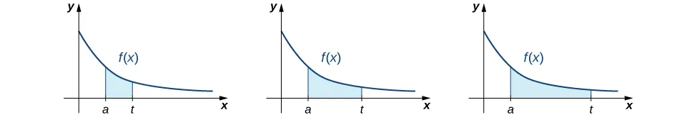
Figure 3\.17 To integrate a function over an infinite interval, we consider the limit of the integral as the upper limit increases without bound.
### Definition
1. Let
𝑓
(
𝑥
)
f
(
x
)
f
(
x
)
be continuous over an interval of the form
\[
𝑎
,
\+
∞
)
.
\[
a
,
\+
∞
)
.
\[
a
,
\+
∞
)
.
Then
∫
\+
∞
𝑎
𝑓
(
𝑥
)
𝑑
𝑥
\=
l
i
m
𝑡
→
\+
∞
∫
𝑡
𝑎
𝑓
(
𝑥
)
𝑑
𝑥
,
∫
a
\+
∞
f
(
x
)
d
x
\=
lim
t
→
\+
∞
∫
a
t
f
(
x
)
d
x
,
∫
a
\+
∞
f
(
x
)
d
x
\=
lim
t
→
\+
∞
∫
a
t
f
(
x
)
d
x
,
(3.16)
provided this limit exists.
2. Let
𝑓
(
𝑥
)
f
(
x
)
f
(
x
)
be continuous over an interval of the form
(
−
∞
,
𝑏
\]
.
(
−
∞
,
b
\]
.
(
−
∞
,
b
\]
.
Then
∫
𝑏
−
∞
𝑓
(
𝑥
)
𝑑
𝑥
\=
l
i
m
𝑡
→
−
∞
∫
𝑏
𝑡
𝑓
(
𝑥
)
𝑑
𝑥
,
∫
−
∞
b
f
(
x
)
d
x
\=
lim
t
→
−
∞
∫
t
b
f
(
x
)
d
x
,
∫
−
∞
b
f
(
x
)
d
x
\=
lim
t
→
−
∞
∫
t
b
f
(
x
)
d
x
,
(3.17)
provided this limit exists.
In each case, if the limit exists, then the improper integral is said to converge. If the limit does not exist, then the improper integral is said to diverge.
3. Let
𝑓
(
𝑥
)
f
(
x
)
f
(
x
)
be continuous over
(
−
∞
,
\+
∞
)
.
(
−
∞
,
\+
∞
)
.
(
−
∞
,
\+
∞
)
.
Then
∫
\+
∞
−
∞
𝑓
(
𝑥
)
𝑑
𝑥
\=
∫
0
−
∞
𝑓
(
𝑥
)
𝑑
𝑥
\+
∫
\+
∞
0
𝑓
(
𝑥
)
𝑑
𝑥
,
∫
−
∞
\+
∞
f
(
x
)
d
x
\=
∫
−
∞
0
f
(
x
)
d
x
\+
∫
0
\+
∞
f
(
x
)
d
x
,
∫
−
∞
\+
∞
f
(
x
)
d
x
\=
∫
−
∞
0
f
(
x
)
d
x
\+
∫
0
\+
∞
f
(
x
)
d
x
,
(3.18)
provided that
∫
0
−
∞
𝑓
(
𝑥
)
𝑑
𝑥
∫
−
∞
0
f
(
x
)
d
x
∫
−
∞
0
f
(
x
)
d
x
and
∫
\+
∞
0
𝑓
(
𝑥
)
𝑑
𝑥
∫
0
\+
∞
f
(
x
)
d
x
∫
0
\+
∞
f
(
x
)
d
x
both converge. If either one or both of these two integrals diverge, then
∫
\+
∞
−
∞
𝑓
(
𝑥
)
𝑑
𝑥
∫
−
∞
\+
∞
f
(
x
)
d
x
∫
−
∞
\+
∞
f
(
x
)
d
x
diverges. (It can be shown that, in fact,
∫
\+
∞
−
∞
𝑓
(
𝑥
)
𝑑
𝑥
\=
∫
𝑎
−
∞
𝑓
(
𝑥
)
𝑑
𝑥
\+
∫
\+
∞
𝑎
𝑓
(
𝑥
)
𝑑
𝑥
∫
−
∞
\+
∞
f
(
x
)
d
x
\=
∫
−
∞
a
f
(
x
)
d
x
\+
∫
a
\+
∞
f
(
x
)
d
x
∫
−
∞
\+
∞
f
(
x
)
d
x
\=
∫
−
∞
a
f
(
x
)
d
x
\+
∫
a
\+
∞
f
(
x
)
d
x
for any value of
𝑎
.
)
a
.
)
a
.
)
In our first example, we return to the question we posed at the start of this section: Is the area between the graph of 𝑓 ( 𝑥 ) \= 1 𝑥 f ( x ) \= 1 x f ( x ) \= 1 x and the 𝑥 x x\-axis over the interval \[ 1 , \+ ∞ ) \[ 1 , \+ ∞ ) \[ 1 , \+ ∞ ) finite or infinite?
### Example 3\.47
#### Finding an Area
Determine whether the area between the graph of 𝑓 ( 𝑥 ) \= 1 𝑥 f ( x ) \= 1 x f ( x ) \= 1 x and the *x*\-axis over the interval \[ 1 , \+ ∞ ) \[ 1 , \+ ∞ ) \[ 1 , \+ ∞ ) is finite or infinite.
#### Solution
We first do a quick sketch of the region in question, as shown in the following graph.
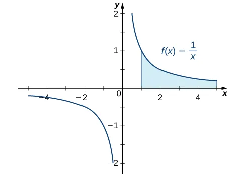
Figure 3\.18
We can find the area between the curve
𝑓
(
𝑥
)
\=
1
/
𝑥
f
(
x
)
\=
1
/
x
f
(
x
)
\=
1
/
x
and the *x*\-axis on an infinite interval.
We can see that the area of this region is given by 𝐴 \= ∫ ∞ 1 1 𝑥 𝑑 𝑥 . A \= ∫ 1 ∞ 1 x d x . A \= ∫ 1 ∞ 1 x d x . Then we have
𝐴
\=
∫
∞
1
1
𝑥
𝑑
𝑥
\=
l
i
m
𝑡
→
\+
∞
∫
𝑡
1
1
𝑥
𝑑
𝑥
R
e
w
r
i
t
e
t
h
e
i
m
p
r
o
p
e
r
i
n
t
e
g
r
a
l
a
s
a
l
i
m
i
t
.
\=
l
i
m
𝑡
→
\+
∞
l
n
\|
𝑥
\|
∣
𝑡
1
F
i
n
d
t
h
e
a
n
t
i
d
e
r
i
v
a
t
i
v
e
.
\=
l
i
m
𝑡
→
\+
∞
(
l
n
\|
𝑡
\|
−
l
n
1
)
E
v
a
l
u
a
t
e
t
h
e
a
n
t
i
d
e
r
i
v
a
t
i
v
e
.
\=
\+
∞
.
E
v
a
l
u
a
t
e
t
h
e
l
i
m
i
t
.
A
\=
∫
1
∞
1
x
d
x
\=
lim
t
→
\+
∞
∫
1
t
1
x
d
x
Rewrite the improper integral as a limit.
\=
lim
t
→
\+
∞
ln
\|
x
\|
\|
1
t
Find the antiderivative.
\=
lim
t
→
\+
∞
(
ln
\|
t
\|
−
ln
1
)
Evaluate the antiderivative.
\=
\+
∞
.
Evaluate the limit.
A
\=
∫
1
∞
1
x
d
x
\=
lim
t
→
\+
∞
∫
1
t
1
x
d
x
Rewrite the improper integral as a limit.
\=
lim
t
→
\+
∞
ln
\|
x
\|
\|
1
t
Find the antiderivative.
\=
lim
t
→
\+
∞
(
ln
\|
t
\|
−
ln
1
)
Evaluate the antiderivative.
\=
\+
∞
.
Evaluate the limit.
Since the improper integral diverges to \+ ∞ , \+ ∞ , \+ ∞ , the area of the region is infinite.
### Example 3\.48
#### Finding a Volume
Find the volume of the solid obtained by revolving the region bounded by the graph of 𝑓 ( 𝑥 ) \= 1 𝑥 f ( x ) \= 1 x f ( x ) \= 1 x and the *x*\-axis over the interval \[ 1 , \+ ∞ ) \[ 1 , \+ ∞ ) \[ 1 , \+ ∞ ) about the 𝑥 x x\-axis.
#### Solution
The solid is shown in [Figure 3.19](https://openstax.org/books/calculus-volume-2/pages/3-7-improper-integrals#CNX_Calc_Figure_07_07_003). Using the disk method, we see that the volume *V* is
𝑉
\=
𝜋
∫
\+
∞
1
1
𝑥
2
𝑑
𝑥
.
V
\=
π
∫
1
\+
∞
1
x
2
d
x
.
V
\=
π
∫
1
\+
∞
1
x
2
d
x
.
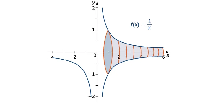
Figure 3\.19 The solid of revolution can be generated by rotating an infinite area about the *x*\-axis.
Then we have
𝑉
\=
𝜋
∫
\+
∞
1
1
𝑥
2
𝑑
𝑥
\=
𝜋
l
i
m
𝑡
→
\+
∞
∫
𝑡
1
1
𝑥
2
𝑑
𝑥
R
e
w
r
i
t
e
a
s
a
l
i
m
i
t
.
\=
𝜋
l
i
m
𝑡
→
\+
∞
−
1
𝑥
∣
𝑡
1
F
i
n
d
t
h
e
a
n
t
i
d
e
r
i
v
a
t
i
v
e
.
\=
𝜋
l
i
m
𝑡
→
\+
∞
(
−
1
𝑡
\+
1
)
E
v
a
l
u
a
t
e
t
h
e
a
n
t
i
d
e
r
i
v
a
t
i
v
e
.
\=
𝜋
.
V
\=
π
∫
1
\+
∞
1
x
2
d
x
\=
π
lim
t
→
\+
∞
∫
1
t
1
x
2
d
x
Rewrite as a limit.
\=
π
lim
t
→
\+
∞
−
1
x
\|
1
t
Find the antiderivative.
\=
π
lim
t
→
\+
∞
(
−
1
t
\+
1
)
Evaluate the antiderivative.
\=
π
.
V
\=
π
∫
1
\+
∞
1
x
2
d
x
\=
π
lim
t
→
\+
∞
∫
1
t
1
x
2
d
x
Rewrite as a limit.
\=
π
lim
t
→
\+
∞
−
1
x
\|
1
t
Find the antiderivative.
\=
π
lim
t
→
\+
∞
(
−
1
t
\+
1
)
Evaluate the antiderivative.
\=
π
.
The improper integral converges to 𝜋 . π . π . Therefore, the volume of the solid of revolution is 𝜋 . π . π .
In conclusion, although the area of the region between the *x*\-axis and the graph of 𝑓 ( 𝑥 ) \= 1 / 𝑥 f ( x ) \= 1 / x f ( x ) \= 1 / x over the interval \[ 1 , \+ ∞ ) \[ 1 , \+ ∞ ) \[ 1 , \+ ∞ ) is infinite, the volume of the solid generated by revolving this region about the *x*\-axis is finite. The solid generated is known as *Gabriel’s Horn*.
### Media
Visit this [website](http://www.openstax.org/l/20_GabrielsHorn) to read more about Gabriel’s Horn.
### Example 3\.49
#### Chapter Opener: Traffic Accidents in a City

Figure 3\.20 (credit: modification of work by David McKelvey, Flickr)
In the chapter opener, we stated the following problem: Suppose that at a busy intersection, traffic accidents occur at an average rate of one every three months. After residents complained, changes were made to the traffic lights at the intersection. It has now been ten months since the changes were made and there have been no accidents. Were the changes effective or is the 10-month interval without an accident a result of chance?
#### Solution
Revise to: Let 𝑥 x x represent the amount of time it takes for the next accident to occur. We want to know how likely it is that 𝑥 \> 1 0 x \> 10 x \> 10. Define the rate parameter λ λ λ to be the average number of accidents per month. According to probability theory, for 𝑎 \> 0 a \> 0 a \> 0,
𝑃
(
𝑥
\>
𝑎
)
\=
∫
∞
𝑎
𝜆
𝑒
−
𝜆
𝑥
𝑑
𝑥
,
P
(
x
\>
a
)
\=
∫
a
∞
λ
e
\-
λ
x
d
x
,
P
x
\>
a
\=
∫
a
∞
λ
e
\-
λ
x
d
x
,
In this example, since one accident happens every three months, on average, λ \= 1 3 λ \= 1 3 λ \= 1 3. The desired probability is:
𝑃
(
𝑥
\>
1
0
)
\=
∫
∞
1
0
1
3
𝑒
−
1
3
𝑥
𝑑
𝑥
\=
l
i
m
𝑡
→
∞
∫
𝑡
1
0
1
3
𝑒
−
1
3
𝑥
𝑑
𝑥
\=
l
i
m
𝑡
→
∞
−
𝑒
−
1
3
𝑥
\|
𝑡
1
0
\=
l
i
m
𝑡
→
∞
(
−
𝑒
−
𝑡
3
\+
𝑒
−
1
0
3
)
≈
0
.
0
3
5
7
P
(
x
\>
10
)
\=
∫
10
∞
1
3
e
−
1
3
x
d
x
\=
lim
t
→
∞
∫
10
t
1
3
e
−
1
3
x
d
x
\=
lim
t
→
∞
−
e
−
1
3
x
\|
10
t
\=
lim
t
→
∞
(
−
e
−
t
3
\+
e
−
10
3
)
≈
0\.0357
P
(
x
\>
10
)
\=
∫
10
∞
1
3
e
−
1
3
x
d
x
\=
lim
t
→
∞
∫
10
t
1
3
e
−
1
3
x
d
x
\=
lim
t
→
∞
−
e
−
1
3
x
\|
10
t
\=
lim
t
→
∞
(
−
e
−
t
3
\+
e
−
10
3
)
≈
0\.0357
The value 3 . 8 × 1 0 − 1 1 3\.8 × 10 −11 3\.8 × 10 −11 represents the probability of no accidents in 8 months under the initial conditions. Since this value is very, very small, it is reasonable to conclude the changes were effective.
### Example 3\.50
#### Evaluating an Improper Integral over an Infinite Interval
Evaluate ∫ 0 − ∞ 1 𝑥 2 \+ 4 𝑑 𝑥 . ∫ − ∞ 0 1 x 2 \+ 4 d x . ∫ − ∞ 0 1 x 2 \+ 4 d x . State whether the improper integral converges or diverges.
#### Solution
Begin by rewriting ∫ 0 − ∞ 1 𝑥 2 \+ 4 𝑑 𝑥 ∫ − ∞ 0 1 x 2 \+ 4 d x ∫ − ∞ 0 1 x 2 \+ 4 d x as a limit using [Equation 3.17](https://openstax.org/books/calculus-volume-2/pages/3-7-improper-integrals#fs-id1165043086270) from the definition. Thus,
∫
0
−
∞
1
𝑥
2
\+
4
𝑑
𝑥
\=
l
i
m
𝑥
→
−
∞
∫
0
𝑡
1
𝑥
2
\+
4
𝑑
𝑥
R
e
w
r
i
t
e
a
s
a
l
i
m
i
t
.
\=
l
i
m
𝑡
→
−
∞
1
2
t
a
n
−
1
𝑥
2
∣
0
𝑡
F
i
n
d
t
h
e
a
n
t
i
d
e
r
i
v
a
t
i
v
e
.
\=
1
2
l
i
m
𝑡
→
−
∞
(
t
a
n
−
1
0
−
t
a
n
−
1
𝑡
2
)
E
v
a
l
u
a
t
e
t
h
e
a
n
t
i
d
e
r
i
v
a
t
i
v
e
.
\=
𝜋
4
.
E
v
a
l
u
a
t
e
t
h
e
l
i
m
i
t
a
n
d
s
i
m
p
l
i
f
y
.
∫
−
∞
0
1
x
2
\+
4
d
x
\=
lim
x
→
−
∞
∫
t
0
1
x
2
\+
4
d
x
Rewrite as a limit.
\=
lim
t
→
−
∞
1
2
tan
−1
x
2
\|
t
0
Find the antiderivative.
\=
1
2
lim
t
→
−
∞
(
tan
−1
0
−
tan
−1
t
2
)
Evaluate the antiderivative.
\=
π
4
.
Evaluate the limit and simplify.
∫
−
∞
0
1
x
2
\+
4
d
x
\=
lim
x
→
−
∞
∫
t
0
1
x
2
\+
4
d
x
Rewrite as a limit.
\=
lim
t
→
−
∞
1
2
tan
−1
x
2
\|
t
0
Find the antiderivative.
\=
1
2
lim
t
→
−
∞
(
tan
−1
0
−
tan
−1
t
2
)
Evaluate the antiderivative.
\=
π
4
.
Evaluate the limit and simplify.
The improper integral converges to 𝜋 4 . π 4 . π 4 .
### Example 3\.51
#### Evaluating an Improper Integral on ( − ∞ , \+ ∞ ) ( − ∞ , \+ ∞ ) ( − ∞ , \+ ∞ )
Evaluate ∫ \+ ∞ − ∞ 𝑥 𝑒 𝑥 𝑑 𝑥 . ∫ − ∞ \+ ∞ x e x d x . ∫ − ∞ \+ ∞ x e x d x . State whether the improper integral converges or diverges.
#### Solution
Start by splitting up the integral:
∫
\+
∞
−
∞
𝑥
𝑒
𝑥
𝑑
𝑥
\=
∫
0
−
∞
𝑥
𝑒
𝑥
𝑑
𝑥
\+
∫
\+
∞
0
𝑥
𝑒
𝑥
𝑑
𝑥
.
∫
−
∞
\+
∞
x
e
x
d
x
\=
∫
−
∞
0
x
e
x
d
x
\+
∫
0
\+
∞
x
e
x
d
x
.
∫
−
∞
\+
∞
x
e
x
d
x
\=
∫
−
∞
0
x
e
x
d
x
\+
∫
0
\+
∞
x
e
x
d
x
.
If either ∫ 0 − ∞ 𝑥 𝑒 𝑥 𝑑 𝑥 ∫ − ∞ 0 x e x d x ∫ − ∞ 0 x e x d x or ∫ \+ ∞ 0 𝑥 𝑒 𝑥 𝑑 𝑥 ∫ 0 \+ ∞ x e x d x ∫ 0 \+ ∞ x e x d x diverges, then ∫ \+ ∞ − ∞ 𝑥 𝑒 𝑥 𝑑 𝑥 ∫ − ∞ \+ ∞ x e x d x ∫ − ∞ \+ ∞ x e x d x diverges. Compute each integral separately. For the first integral,
∫
0
−
∞
𝑥
𝑒
𝑥
𝑑
𝑥
\=
l
i
m
𝑡
→
−
∞
∫
0
𝑡
𝑥
𝑒
𝑥
𝑑
𝑥
R
e
w
r
i
t
e
a
s
a
l
i
m
i
t
.
\=
l
i
m
𝑡
→
−
∞
(
𝑥
𝑒
𝑥
−
𝑒
𝑥
)
∣
0
𝑡
U
s
e
i
n
t
e
g
r
a
t
i
o
n
b
y
p
a
r
t
s
t
o
f
i
n
d
t
h
e
a
n
t
i
d
e
r
i
v
a
t
i
v
e
.
(
H
e
r
e
𝑢
\=
𝑥
a
n
d
𝑑
𝑣
\=
𝑒
𝑥
d
x
.
)
\=
l
i
m
𝑡
→
−
∞
(
−
1
−
𝑡
𝑒
𝑡
\+
𝑒
𝑡
)
E
v
a
l
u
a
t
e
t
h
e
a
n
t
i
d
e
r
i
v
a
t
i
v
e
.
\=
−
1
.
E
v
a
l
u
a
t
e
t
h
e
l
i
m
i
t
.
𝑁
𝑜
𝑡
𝑒
:
l
i
m
𝑡
→
−
∞
𝑡
𝑒
𝑡
i
s
i
n
d
e
t
e
r
m
i
n
a
t
e
o
f
t
h
e
f
o
r
m
0
·
∞
.
T
h
u
s
,
l
i
m
𝑡
→
−
∞
𝑡
𝑒
𝑡
\=
l
i
m
𝑡
→
−
∞
𝑡
𝑒
−
𝑡
\=
l
i
m
𝑡
→
−
∞
−
1
𝑒
−
𝑡
\=
l
i
m
𝑡
→
−
∞
−
𝑒
𝑡
\=
0
b
y
L
’
H
ô
p
i
t
a
l
’
s
R
u
l
e
.
∫
−
∞
0
x
e
x
d
x
\=
lim
t
→
−
∞
∫
t
0
x
e
x
d
x
Rewrite as a limit.
\=
lim
t
→
−
∞
(
x
e
x
−
e
x
)
\|
t
0
Use integration by parts to find the
antiderivative. (Here
u
\=
x
and
d
v
\=
e
x
dx
.
)
\=
lim
t
→
−
∞
(
−1
−
t
e
t
\+
e
t
)
Evaluate the antiderivative.
\=
−1
.
Evaluate the limit.
Note:
lim
t
→
−
∞
t
e
t
is
indeterminate of the form
0
·
∞
.
Thus,
lim
t
→
−
∞
t
e
t
\=
lim
t
→
−
∞
t
e
−
t
\=
lim
t
→
−
∞
−1
e
−
t
\=
lim
t
→
−
∞
−
e
t
\=
0
by
L’Hôpital’s Rule.
∫
−
∞
0
x
e
x
d
x
\=
lim
t
→
−
∞
∫
t
0
x
e
x
d
x
Rewrite as a limit.
\=
lim
t
→
−
∞
(
x
e
x
−
e
x
)
\|
t
0
Use integration by parts to find the
antiderivative. (Here
u
\=
x
and
d
v
\=
e
x
dx
.
)
\=
lim
t
→
−
∞
(
−1
−
t
e
t
\+
e
t
)
Evaluate the antiderivative.
\=
−1
.
Evaluate the limit.
Note:
lim
t
→
−
∞
t
e
t
is
indeterminate of the form
0
·
∞
.
Thus,
lim
t
→
−
∞
t
e
t
\=
lim
t
→
−
∞
t
e
−
t
\=
lim
t
→
−
∞
−1
e
−
t
\=
lim
t
→
−
∞
−
e
t
\=
0
by
L’Hôpital’s Rule.
The first improper integral converges. For the second integral,
∫
\+
∞
0
𝑥
𝑒
𝑥
𝑑
𝑥
\=
l
i
m
𝑡
→
\+
∞
∫
𝑡
0
𝑥
𝑒
𝑥
𝑑
𝑥
R
e
w
r
i
t
e
a
s
a
l
i
m
i
t
.
\=
l
i
m
𝑡
→
\+
∞
(
𝑥
𝑒
𝑥
−
𝑒
𝑥
)
∣
𝑡
0
F
i
n
d
t
h
e
a
n
t
i
d
e
r
i
v
a
t
i
v
e
.
\=
l
i
m
𝑡
→
\+
∞
(
𝑡
𝑒
𝑡
−
𝑒
𝑡
\+
1
)
E
v
a
l
u
a
t
e
t
h
e
a
n
t
i
d
e
r
i
v
a
t
i
v
e
.
\=
l
i
m
𝑡
→
\+
∞
(
(
𝑡
−
1
)
𝑒
𝑡
\+
1
)
R
e
w
r
i
t
e
.
(
𝑡
𝑒
𝑡
−
𝑒
𝑡
i
s
i
n
d
e
t
e
r
m
i
n
a
t
e
.
)
\=
\+
∞
.
E
v
a
l
u
a
t
e
t
h
e
l
i
m
i
t
.
∫
0
\+
∞
x
e
x
d
x
\=
lim
t
→
\+
∞
∫
0
t
x
e
x
d
x
Rewrite as a limit.
\=
lim
t
→
\+
∞
(
x
e
x
−
e
x
)
\|
0
t
Find the antiderivative.
\=
lim
t
→
\+
∞
(
t
e
t
−
e
t
\+
1
)
Evaluate the antiderivative.
\=
lim
t
→
\+
∞
(
(
t
−
1
)
e
t
\+
1
)
Rewrite.
(
t
e
t
−
e
t
is indeterminate.)
\=
\+
∞
.
Evaluate the limit.
∫
0
\+
∞
x
e
x
d
x
\=
lim
t
→
\+
∞
∫
0
t
x
e
x
d
x
Rewrite as a limit.
\=
lim
t
→
\+
∞
(
x
e
x
−
e
x
)
\|
0
t
Find the antiderivative.
\=
lim
t
→
\+
∞
(
t
e
t
−
e
t
\+
1
)
Evaluate the antiderivative.
\=
lim
t
→
\+
∞
(
(
t
−
1
)
e
t
\+
1
)
Rewrite.
(
t
e
t
−
e
t
is indeterminate.)
\=
\+
∞
.
Evaluate the limit.
Thus, ∫ \+ ∞ 0 𝑥 𝑒 𝑥 𝑑 𝑥 ∫ 0 \+ ∞ x e x d x ∫ 0 \+ ∞ x e x d x diverges. Since this integral diverges, ∫ \+ ∞ − ∞ 𝑥 𝑒 𝑥 𝑑 𝑥 ∫ − ∞ \+ ∞ x e x d x ∫ − ∞ \+ ∞ x e x d x diverges as well.
### Checkpoint 3\.27
Evaluate ∫ \+ ∞ − 3 𝑒 − 𝑥 𝑑 𝑥 . ∫ −3 \+ ∞ e − x d x . ∫ −3 \+ ∞ e − x d x . State whether the improper integral converges or diverges.
### Integrating a Discontinuous Integrand
Now let’s examine integrals of functions containing an infinite discontinuity in the interval over which the integration occurs. Consider an integral of the form ∫ 𝑏 𝑎 𝑓 ( 𝑥 ) 𝑑 𝑥 , ∫ a b f ( x ) d x , ∫ a b f ( x ) d x , where 𝑓 ( 𝑥 ) f ( x ) f ( x ) is continuous over \[ 𝑎 , 𝑏 ) \[ a , b ) \[ a , b ) and discontinuous at 𝑏 . b . b . Since the function 𝑓 ( 𝑥 ) f ( x ) f ( x ) is continuous over \[ 𝑎 , 𝑡 \] \[ a , t \] \[ a , t \] for all values of 𝑡 t t satisfying 𝑎 \< 𝑡 \< 𝑏 , a \< t \< b , a \< t \< b , the integral ∫ 𝑡 𝑎 𝑓 ( 𝑥 ) 𝑑 𝑥 ∫ a t f ( x ) d x ∫ a t f ( x ) d x is defined for all such values of 𝑡 . t . t . Thus, it makes sense to consider the values of ∫ 𝑡 𝑎 𝑓 ( 𝑥 ) 𝑑 𝑥 ∫ a t f ( x ) d x ∫ a t f ( x ) d x as 𝑡 t t approaches 𝑏 b b for 𝑎 \< 𝑡 \< 𝑏 . a \< t \< b . a \< t \< b . That is, we define ∫ 𝑏 𝑎 𝑓 ( 𝑥 ) 𝑑 𝑥 \= l i m 𝑡 → 𝑏 − ∫ 𝑡 𝑎 𝑓 ( 𝑥 ) 𝑑 𝑥 , ∫ a b f ( x ) d x \= lim t → b − ∫ a t f ( x ) d x , ∫ a b f ( x ) d x \= lim t → b − ∫ a t f ( x ) d x , provided this limit exists. [Figure 3.21](https://openstax.org/books/calculus-volume-2/pages/3-7-improper-integrals#CNX_Calc_Figure_07_07_004) illustrates ∫ 𝑡 𝑎 𝑓 ( 𝑥 ) 𝑑 𝑥 ∫ a t f ( x ) d x ∫ a t f ( x ) d x as areas of regions for values of 𝑡 t t approaching 𝑏 . b . b .
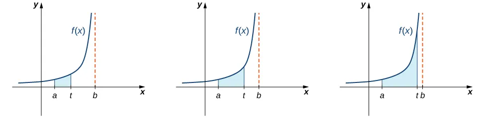
Figure 3\.21 As *t* approaches *b* from the left, the value of the area from *a* to *t* approaches the area from *a* to *b*.
We use a similar approach to define ∫ 𝑏 𝑎 𝑓 ( 𝑥 ) 𝑑 𝑥 , ∫ a b f ( x ) d x , ∫ a b f ( x ) d x , where 𝑓 ( 𝑥 ) f ( x ) f ( x ) is continuous over ( 𝑎 , 𝑏 \] ( a , b \] ( a , b \] and discontinuous at 𝑎 . a . a . We now proceed with a formal definition.
### Definition
1. Let
𝑓
(
𝑥
)
f
(
x
)
f
(
x
)
be continuous over
\[
𝑎
,
𝑏
)
.
\[
a
,
b
)
.
\[
a
,
b
)
.
Then,
∫
𝑏
𝑎
𝑓
(
𝑥
)
𝑑
𝑥
\=
l
i
m
𝑡
→
𝑏
−
∫
𝑡
𝑎
𝑓
(
𝑥
)
𝑑
𝑥
.
∫
a
b
f
(
x
)
d
x
\=
lim
t
→
b
−
∫
a
t
f
(
x
)
d
x
.
∫
a
b
f
(
x
)
d
x
\=
lim
t
→
b
−
∫
a
t
f
(
x
)
d
x
.
(3.19)
2. Let
𝑓
(
𝑥
)
f
(
x
)
f
(
x
)
be continuous over
(
𝑎
,
𝑏
\]
.
(
a
,
b
\]
.
(
a
,
b
\]
.
Then,
∫
𝑏
𝑎
𝑓
(
𝑥
)
𝑑
𝑥
\=
l
i
m
𝑡
→
𝑎
\+
∫
𝑏
𝑡
𝑓
(
𝑥
)
𝑑
𝑥
.
∫
a
b
f
(
x
)
d
x
\=
lim
t
→
a
\+
∫
t
b
f
(
x
)
d
x
.
∫
a
b
f
(
x
)
d
x
\=
lim
t
→
a
\+
∫
t
b
f
(
x
)
d
x
.
(3.20)
In each case, if the limit exists, then the improper integral is said to converge. If the limit does not exist, then the improper integral is said to diverge.
3. If
𝑓
(
𝑥
)
f
(
x
)
f
(
x
)
is continuous over
\[
𝑎
,
𝑏
\]
\[
a
,
b
\]
\[
a
,
b
\]
except at a point
𝑐
c
c
in
(
𝑎
,
𝑏
)
,
(
a
,
b
)
,
(
a
,
b
)
,
then
∫
𝑏
𝑎
𝑓
(
𝑥
)
𝑑
𝑥
\=
∫
𝑐
𝑎
𝑓
(
𝑥
)
𝑑
𝑥
\+
∫
𝑏
𝑐
𝑓
(
𝑥
)
𝑑
𝑥
,
∫
a
b
f
(
x
)
d
x
\=
∫
a
c
f
(
x
)
d
x
\+
∫
c
b
f
(
x
)
d
x
,
∫
a
b
f
(
x
)
d
x
\=
∫
a
c
f
(
x
)
d
x
\+
∫
c
b
f
(
x
)
d
x
,
(3.21)
provided both
∫
𝑐
𝑎
𝑓
(
𝑥
)
𝑑
𝑥
∫
a
c
f
(
x
)
d
x
∫
a
c
f
(
x
)
d
x
and
∫
𝑏
𝑐
𝑓
(
𝑥
)
𝑑
𝑥
∫
c
b
f
(
x
)
d
x
∫
c
b
f
(
x
)
d
x
converge. If either of these integrals diverges, then
∫
𝑏
𝑎
𝑓
(
𝑥
)
𝑑
𝑥
∫
a
b
f
(
x
)
d
x
∫
a
b
f
(
x
)
d
x
diverges.
The following examples demonstrate the application of this definition.
### Example 3\.52
#### Integrating a Discontinuous Integrand
Evaluate ∫ 4 0 1 √ 4 − 𝑥 𝑑 𝑥 , ∫ 0 4 1 4 − x d x , ∫ 0 4 1 4 − x d x , if possible. State whether the integral converges or diverges.
#### Solution
The function 𝑓 ( 𝑥 ) \= 1 √ 4 − 𝑥 f ( x ) \= 1 4 − x f ( x ) \= 1 4 − x is continuous over \[ 0 , 4 ) \[ 0 , 4 ) \[ 0 , 4 ) and discontinuous at 4. Using [Equation 3.19](https://openstax.org/books/calculus-volume-2/pages/3-7-improper-integrals#fs-id1165042617693) from the definition, rewrite ∫ 4 0 1 √ 4 − 𝑥 𝑑 𝑥 ∫ 0 4 1 4 − x d x ∫ 0 4 1 4 − x d x as a limit:
∫
4
0
1
√
4
−
𝑥
𝑑
𝑥
\=
l
i
m
𝑡
→
4
−
∫
𝑡
0
1
√
4
−
𝑥
𝑑
𝑥
R
e
w
r
i
t
e
a
s
a
l
i
m
i
t
.
\=
l
i
m
𝑡
→
4
−
(
−
2
√
4
−
𝑥
)
∣
𝑡
0
F
i
n
d
t
h
e
a
n
t
i
d
e
r
i
v
a
t
i
v
e
.
\=
l
i
m
𝑡
→
4
−
(
−
2
√
4
−
𝑡
\+
4
)
E
v
a
l
u
a
t
e
t
h
e
a
n
t
i
d
e
r
i
v
a
t
i
v
e
.
\=
4
.
E
v
a
l
u
a
t
e
t
h
e
l
i
m
i
t
.
∫
0
4
1
4
−
x
d
x
\=
lim
t
→
4
−
∫
0
t
1
4
−
x
d
x
Rewrite as a limit.
\=
lim
t
→
4
−
(
−2
4
−
x
)
\|
0
t
Find the antiderivative.
\=
lim
t
→
4
−
(
−2
4
−
t
\+
4
)
Evaluate the antiderivative.
\=
4
.
Evaluate the limit.
∫
0
4
1
4
−
x
d
x
\=
lim
t
→
4
−
∫
0
t
1
4
−
x
d
x
Rewrite as a limit.
\=
lim
t
→
4
−
(
−2
4
−
x
)
\|
0
t
Find the antiderivative.
\=
lim
t
→
4
−
(
−2
4
−
t
\+
4
)
Evaluate the antiderivative.
\=
4
.
Evaluate the limit.
The improper integral converges.
### Example 3\.53
#### Integrating a Discontinuous Integrand
Evaluate ∫ 2 0 𝑥 l n 𝑥 𝑑 𝑥 . ∫ 0 2 x ln x d x . ∫ 0 2 x ln x d x . State whether the integral converges or diverges.
#### Solution
Since 𝑓 ( 𝑥 ) \= 𝑥 l n 𝑥 f ( x ) \= x ln x f ( x ) \= x ln x is continuous over ( 0 , 2 \] ( 0 , 2 \] ( 0 , 2 \] and is discontinuous at zero, we can rewrite the integral in limit form using [Equation 3.20](https://openstax.org/books/calculus-volume-2/pages/3-7-improper-integrals#fs-id1165042506827):
∫
2
0
𝑥
l
n
𝑥
𝑑
𝑥
\=
l
i
m
𝑡
→
0
\+
∫
2
𝑡
𝑥
l
n
𝑥
𝑑
𝑥
R
e
w
r
i
t
e
a
s
a
l
i
m
i
t
.
\=
l
i
m
𝑡
→
0
\+
(
1
2
𝑥
2
l
n
𝑥
−
1
4
𝑥
2
)
∣
2
𝑡
E
v
a
l
u
a
t
e
∫
𝑥
l
n
𝑥
𝑑
𝑥
u
s
i
n
g
i
n
t
e
g
r
a
t
i
o
n
b
y
p
a
r
t
s
w
i
t
h
𝑢
\=
l
n
𝑥
a
n
d
𝑑
𝑣
\=
𝑥
d
x
.
\=
l
i
m
𝑡
→
0
\+
(
2
l
n
2
−
1
−
1
2
𝑡
2
l
n
𝑡
\+
1
4
𝑡
2
)
.
E
v
a
l
u
a
t
e
t
h
e
a
n
t
i
d
e
r
i
v
a
t
i
v
e
.
\=
2
l
n
2
−
1
.
E
v
a
l
u
a
t
e
t
h
e
l
i
m
i
t
.
l
i
m
𝑡
→
0
\+
𝑡
2
l
n
𝑡
i
s
i
n
d
e
t
e
r
m
i
n
a
t
e
.
T
o
e
v
a
l
u
a
t
e
i
t
,
r
e
w
r
i
t
e
a
s
a
q
u
o
t
i
e
n
t
a
n
d
a
p
p
l
y
L
’
H
ô
p
i
t
a
l
’
s
r
u
l
e
.
∫
0
2
x
ln
x
d
x
\=
lim
t
→
0
\+
∫
t
2
x
ln
x
d
x
Rewrite as a limit.
\=
lim
t
→
0
\+
(
1
2
x
2
ln
x
−
1
4
x
2
)
\|
t
2
Evaluate
∫
x
ln
x
d
x
using integration by parts
with
u
\=
ln
x
and
d
v
\=
x
dx
.
\=
lim
t
→
0
\+
(
2
ln
2
−
1
−
1
2
t
2
ln
t
\+
1
4
t
2
)
.
Evaluate the antiderivative.
\=
2
ln
2
−
1
.
Evaluate the limit.
lim
t
→
0
\+
t
2
ln
t
is indeterminate.
To evaluate it, rewrite as a quotient and apply
L’Hôpital’s rule.
∫
0
2
x
ln
x
d
x
\=
lim
t
→
0
\+
∫
t
2
x
ln
x
d
x
Rewrite as a limit.
\=
lim
t
→
0
\+
(
1
2
x
2
ln
x
−
1
4
x
2
)
\|
t
2
Evaluate
∫
x
ln
x
d
x
using integration by parts
with
u
\=
ln
x
and
d
v
\=
x
dx
.
\=
lim
t
→
0
\+
(
2
ln
2
−
1
−
1
2
t
2
ln
t
\+
1
4
t
2
)
.
Evaluate the antiderivative.
\=
2
ln
2
−
1
.
Evaluate the limit.
lim
t
→
0
\+
t
2
ln
t
is indeterminate.
To evaluate it, rewrite as a quotient and apply
L’Hôpital’s rule.
The improper integral converges.
### Example 3\.54
#### Integrating a Discontinuous Integrand
Evaluate ∫ 1 − 1 1 𝑥 3 𝑑 𝑥 . ∫ −1 1 1 x 3 d x . ∫ −1 1 1 x 3 d x . State whether the improper integral converges or diverges.
#### Solution
Since 𝑓 ( 𝑥 ) \= 1 / 𝑥 3 f ( x ) \= 1 / x 3 f ( x ) \= 1 / x 3 is discontinuous at zero, using [Equation 3.21](https://openstax.org/books/calculus-volume-2/pages/3-7-improper-integrals#fs-id1165043378015), we can write
∫
1
−
1
1
𝑥
3
𝑑
𝑥
\=
∫
0
−
1
1
𝑥
3
𝑑
𝑥
\+
∫
1
0
1
𝑥
3
𝑑
𝑥
.
∫
−1
1
1
x
3
d
x
\=
∫
−1
0
1
x
3
d
x
\+
∫
0
1
1
x
3
d
x
.
∫
−1
1
1
x
3
d
x
\=
∫
−1
0
1
x
3
d
x
\+
∫
0
1
1
x
3
d
x
.
If either of the two integrals diverges, then the original integral diverges. Begin with ∫ 0 − 1 1 𝑥 3 𝑑 𝑥 : ∫ −1 0 1 x 3 d x : ∫ −1 0 1 x 3 d x :
∫
0
−
1
1
𝑥
3
𝑑
𝑥
\=
l
i
m
𝑡
→
0
−
∫
𝑡
−
1
1
𝑥
3
𝑑
𝑥
R
e
w
r
i
t
e
a
s
a
l
i
m
i
t
.
\=
l
i
m
𝑡
→
0
−
(
−
1
2
𝑥
2
)
∣
𝑡
−
1
F
i
n
d
t
h
e
a
n
t
i
d
e
r
i
v
a
t
i
v
e
.
\=
l
i
m
𝑡
→
0
−
(
−
1
2
𝑡
2
\+
1
2
)
E
v
a
l
u
a
t
e
t
h
e
a
n
t
i
d
e
r
i
v
a
t
i
v
e
.
\=
\+
–
∞
.
E
v
a
l
u
a
t
e
t
h
e
l
i
m
i
t
.
∫
−1
0
1
x
3
d
x
\=
lim
t
→
0
−
∫
−1
t
1
x
3
d
x
Rewrite as a limit.
\=
lim
t
→
0
−
(
−
1
2
x
2
)
\|
−1
t
Find the antiderivative.
\=
lim
t
→
0
−
(
−
1
2
t
2
\+
1
2
)
Evaluate the antiderivative.
\=
\+
–∞
.
Evaluate the limit.
∫
−1
0
1
x
3
d
x
\=
lim
t
→
0
−
∫
−1
t
1
x
3
d
x
Rewrite as a limit.
\=
lim
t
→
0
−
(
−
1
2
x
2
)
\|
−1
t
Find the antiderivative.
\=
lim
t
→
0
−
(
−
1
2
t
2
\+
1
2
)
Evaluate the antiderivative.
\=
\+
–∞
.
Evaluate the limit.
Therefore, ∫ 0 − 1 1 𝑥 3 𝑑 𝑥 ∫ −1 0 1 x 3 d x ∫ −1 0 1 x 3 d x diverges. Since ∫ 0 − 1 1 𝑥 3 𝑑 𝑥 ∫ −1 0 1 x 3 d x ∫ −1 0 1 x 3 d x diverges, ∫ 1 − 1 1 𝑥 3 𝑑 𝑥 ∫ −1 1 1 x 3 d x ∫ −1 1 1 x 3 d x diverges.
### Checkpoint 3\.28
Evaluate ∫ 2 0 1 𝑥 𝑑 𝑥 . ∫ 0 2 1 x d x . ∫ 0 2 1 x d x . State whether the integral converges or diverges.
### A Comparison Theorem
It is not always easy or even possible to evaluate an improper integral directly; however, by comparing it with another carefully chosen integral, it may be possible to determine its convergence or divergence. To see this, consider two continuous functions 𝑓 ( 𝑥 ) f ( x ) f ( x ) and 𝑔 ( 𝑥 ) g ( x ) g ( x ) satisfying 0 ≤ 𝑓 ( 𝑥 ) ≤ 𝑔 ( 𝑥 ) 0 ≤ f ( x ) ≤ g ( x ) 0 ≤ f ( x ) ≤ g ( x ) for 𝑥 ≥ 𝑎 x ≥ a x ≥ a ([Figure 3.22](https://openstax.org/books/calculus-volume-2/pages/3-7-improper-integrals#CNX_Calc_Figure_07_07_005)). In this case, we may view integrals of these functions over intervals of the form \[ 𝑎 , 𝑡 \] \[ a , t \] \[ a , t \] as areas, so we have the relationship
0
≤
∫
𝑡
𝑎
𝑓
(
𝑥
)
𝑑
𝑥
≤
∫
𝑡
𝑎
𝑔
(
𝑥
)
𝑑
𝑥
f
o
r
𝑡
≥
𝑎
.
0
≤
∫
a
t
f
(
x
)
d
x
≤
∫
a
t
g
(
x
)
d
x
for
t
≥
a
.
0
≤
∫
a
t
f
(
x
)
d
x
≤
∫
a
t
g
(
x
)
d
x
for
t
≥
a
.
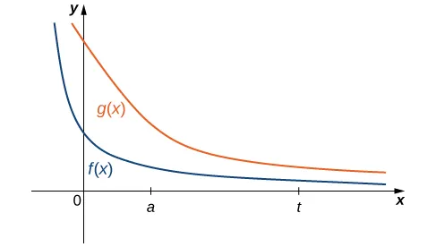
Figure 3\.22
If
0
≤
𝑓
(
𝑥
)
≤
𝑔
(
𝑥
)
0
≤
f
(
x
)
≤
g
(
x
)
0
≤
f
(
x
)
≤
g
(
x
)
for
𝑥
≥
𝑎
,
x
≥
a
,
x
≥
a
,
then for
𝑡
≥
𝑎
,
t
≥
a
,
t
≥
a
,
∫
𝑡
𝑎
𝑓
(
𝑥
)
𝑑
𝑥
≤
∫
𝑡
𝑎
𝑔
(
𝑥
)
𝑑
𝑥
.
∫
a
t
f
(
x
)
d
x
≤
∫
a
t
g
(
x
)
d
x
.
∫
a
t
f
(
x
)
d
x
≤
∫
a
t
g
(
x
)
d
x
.
Thus, if
∫
\+
∞
𝑎
𝑓
(
𝑥
)
𝑑
𝑥
\=
l
i
m
𝑡
→
\+
∞
∫
𝑡
𝑎
𝑓
(
𝑥
)
𝑑
𝑥
\=
\+
∞
,
∫
a
\+
∞
f
(
x
)
d
x
\=
lim
t
→
\+
∞
∫
a
t
f
(
x
)
d
x
\=
\+
∞
,
∫
a
\+
∞
f
(
x
)
d
x
\=
lim
t
→
\+
∞
∫
a
t
f
(
x
)
d
x
\=
\+
∞
,
then
∫ \+ ∞ 𝑎 𝑔 ( 𝑥 ) 𝑑 𝑥 \= l i m 𝑡 → \+ ∞ ∫ 𝑡 𝑎 𝑔 ( 𝑥 ) 𝑑 𝑥 \= \+ ∞ ∫ a \+ ∞ g ( x ) d x \= lim t → \+ ∞ ∫ a t g ( x ) d x \= \+ ∞ ∫ a \+ ∞ g ( x ) d x \= lim t → \+ ∞ ∫ a t g ( x ) d x \= \+ ∞ as well. That is, if the area of the region between the graph of 𝑓 ( 𝑥 ) f ( x ) f ( x ) and the *x*\-axis over \[ 𝑎 , \+ ∞ ) \[ a , \+ ∞ ) \[ a , \+ ∞ ) is infinite, then the area of the region between the graph of 𝑔 ( 𝑥 ) g ( x ) g ( x ) and the *x*\-axis over \[ 𝑎 , \+ ∞ ) \[ a , \+ ∞ ) \[ a , \+ ∞ ) is infinite too.
On the other hand, if
∫ \+ ∞ 𝑎 𝑔 ( 𝑥 ) 𝑑 𝑥 \= l i m 𝑡 → \+ ∞ ∫ 𝑡 𝑎 𝑔 ( 𝑥 ) 𝑑 𝑥 \= 𝐿 ∫ a \+ ∞ g ( x ) d x \= lim t → \+ ∞ ∫ a t g ( x ) d x \= L ∫ a \+ ∞ g ( x ) d x \= lim t → \+ ∞ ∫ a t g ( x ) d x \= L for some real number 𝐿 , L , L , then
∫ \+ ∞ 𝑎 𝑓 ( 𝑥 ) 𝑑 𝑥 \= l i m 𝑡 → \+ ∞ ∫ 𝑡 𝑎 𝑓 ( 𝑥 ) 𝑑 𝑥 ∫ a \+ ∞ f ( x ) d x \= lim t → \+ ∞ ∫ a t f ( x ) d x ∫ a \+ ∞ f ( x ) d x \= lim t → \+ ∞ ∫ a t f ( x ) d x must converge to some value less than or equal to 𝐿 , L , L , since ∫ 𝑡 𝑎 𝑓 ( 𝑥 ) 𝑑 𝑥 ∫ a t f ( x ) d x ∫ a t f ( x ) d x increases as 𝑡 t t increases and ∫ 𝑡 𝑎 𝑓 ( 𝑥 ) 𝑑 𝑥 ≤ 𝐿 ∫ a t f ( x ) d x ≤ L ∫ a t f ( x ) d x ≤ L for all 𝑡 ≥ 𝑎 . t ≥ a . t ≥ a .
If the area of the region between the graph of 𝑔 ( 𝑥 ) g ( x ) g ( x ) and the *x*\-axis over \[ 𝑎 , \+ ∞ ) \[ a , \+ ∞ ) \[ a , \+ ∞ ) is finite, then the area of the region between the graph of 𝑓 ( 𝑥 ) f ( x ) f ( x ) and the *x*\-axis over \[ 𝑎 , \+ ∞ ) \[ a , \+ ∞ ) \[ a , \+ ∞ ) is also finite.
These conclusions are summarized in the following theorem.
### Theorem 3\.7
#### A Comparison Theorem
Let 𝑓 ( 𝑥 ) f ( x ) f ( x ) and 𝑔 ( 𝑥 ) g ( x ) g ( x ) be continuous over \[ 𝑎 , \+ ∞ ) . \[ a , \+ ∞ ) . \[ a , \+ ∞ ) . Assume that 0 ≤ 𝑓 ( 𝑥 ) ≤ 𝑔 ( 𝑥 ) 0 ≤ f ( x ) ≤ g ( x ) 0 ≤ f ( x ) ≤ g ( x ) for 𝑥 ≥ 𝑎 . x ≥ a . x ≥ a .
1. If
∫
\+
∞
𝑎
𝑓
(
𝑥
)
𝑑
𝑥
\=
l
i
m
𝑡
→
\+
∞
∫
𝑡
𝑎
𝑓
(
𝑥
)
𝑑
𝑥
\=
\+
∞
,
∫
a
\+
∞
f
(
x
)
d
x
\=
lim
t
→
\+
∞
∫
a
t
f
(
x
)
d
x
\=
\+
∞
,
∫
a
\+
∞
f
(
x
)
d
x
\=
lim
t
→
\+
∞
∫
a
t
f
(
x
)
d
x
\=
\+
∞
,
then
∫
\+
∞
𝑎
𝑔
(
𝑥
)
𝑑
𝑥
\=
l
i
m
𝑡
→
\+
∞
∫
𝑡
𝑎
𝑔
(
𝑥
)
𝑑
𝑥
\=
\+
∞
.
∫
a
\+
∞
g
(
x
)
d
x
\=
lim
t
→
\+
∞
∫
a
t
g
(
x
)
d
x
\=
\+
∞
.
∫
a
\+
∞
g
(
x
)
d
x
\=
lim
t
→
\+
∞
∫
a
t
g
(
x
)
d
x
\=
\+
∞
.
2. If
∫
\+
∞
𝑎
𝑔
(
𝑥
)
𝑑
𝑥
\=
l
i
m
𝑡
→
\+
∞
∫
𝑡
𝑎
𝑔
(
𝑥
)
𝑑
𝑥
\=
𝐿
,
∫
a
\+
∞
g
(
x
)
d
x
\=
lim
t
→
\+
∞
∫
a
t
g
(
x
)
d
x
\=
L
,
∫
a
\+
∞
g
(
x
)
d
x
\=
lim
t
→
\+
∞
∫
a
t
g
(
x
)
d
x
\=
L
,
where
𝐿
L
L
is a real number, then
∫
\+
∞
𝑎
𝑓
(
𝑥
)
𝑑
𝑥
\=
l
i
m
𝑡
→
\+
∞
∫
𝑡
𝑎
𝑓
(
𝑥
)
𝑑
𝑥
\=
𝑀
∫
a
\+
∞
f
(
x
)
d
x
\=
lim
t
→
\+
∞
∫
a
t
f
(
x
)
d
x
\=
M
∫
a
\+
∞
f
(
x
)
d
x
\=
lim
t
→
\+
∞
∫
a
t
f
(
x
)
d
x
\=
M
for some real number
𝑀
≤
𝐿
.
M
≤
L
.
M
≤
L
.
### Example 3\.55
#### Applying the Comparison Theorem
Use a comparison to show that ∫ \+ ∞ 1 1 𝑥 𝑒 𝑥 𝑑 𝑥 ∫ 1 \+ ∞ 1 x e x d x ∫ 1 \+ ∞ 1 x e x d x converges.
#### Solution
We can see that
0
≤
1
𝑥
𝑒
𝑥
≤
1
𝑒
𝑥
\=
𝑒
−
𝑥
,
0
≤
1
x
e
x
≤
1
e
x
\=
e
−
x
,
0
≤
1
x
e
x
≤
1
e
x
\=
e
−
x
,
so if ∫ \+ ∞ 1 𝑒 − 𝑥 𝑑 𝑥 ∫ 1 \+ ∞ e − x d x ∫ 1 \+ ∞ e − x d x converges, then so does ∫ \+ ∞ 1 1 𝑥 𝑒 𝑥 𝑑 𝑥 . ∫ 1 \+ ∞ 1 x e x d x . ∫ 1 \+ ∞ 1 x e x d x . To evaluate ∫ \+ ∞ 1 𝑒 − 𝑥 𝑑 𝑥 , ∫ 1 \+ ∞ e − x d x , ∫ 1 \+ ∞ e − x d x , first rewrite it as a limit:
∫
\+
∞
1
𝑒
−
𝑥
𝑑
𝑥
\=
l
i
m
𝑡
→
\+
∞
∫
𝑡
1
𝑒
−
𝑥
𝑑
𝑥
\=
l
i
m
𝑡
→
\+
∞
(
−
𝑒
−
𝑥
)
∣
𝑡
1
\=
l
i
m
𝑡
→
\+
∞
(
−
𝑒
−
𝑡
\+
𝑒
–
1
)
\=
𝑒
–
1
.
∫
1
\+
∞
e
−
x
d
x
\=
lim
t
→
\+
∞
∫
1
t
e
−
x
d
x
\=
lim
t
→
\+
∞
(
−
e
−
x
)
\|
t
1
\=
lim
t
→
\+
∞
(
−
e
−
t
\+
e
–1
)
\=
e
–1
.
∫
1
\+
∞
e
−
x
d
x
\=
lim
t
→
\+
∞
∫
1
t
e
−
x
d
x
\=
lim
t
→
\+
∞
(
−
e
−
x
)
\|
t
1
\=
lim
t
→
\+
∞
(
−
e
−
t
\+
e
–1
)
\=
e
–1
.
Since ∫ \+ ∞ 1 𝑒 − 𝑥 𝑑 𝑥 ∫ 1 \+ ∞ e − x d x ∫ 1 \+ ∞ e − x d x converges, so does ∫ \+ ∞ 1 1 𝑥 𝑒 𝑥 𝑑 𝑥 . ∫ 1 \+ ∞ 1 x e x d x . ∫ 1 \+ ∞ 1 x e x d x .
### Example 3\.56
#### Applying the Comparison Theorem
Use the comparison theorem to show that ∫ \+ ∞ 1 1 𝑥 𝑝 𝑑 𝑥 ∫ 1 \+ ∞ 1 x p d x ∫ 1 \+ ∞ 1 x p d x diverges for all 𝑝 \< 1 . p \< 1 . p \< 1 .
#### Solution
For 𝑝 \< 1 , p \< 1 , p \< 1 , 1 / 𝑥 ≤ 1 / ( 𝑥 𝑝 ) 1 / x ≤ 1 / ( x p ) 1 / x ≤ 1 / ( x p ) over \[ 1 , \+ ∞ ) . \[ 1 , \+ ∞ ) . \[ 1 , \+ ∞ ) . In [Example 3.47](https://openstax.org/books/calculus-volume-2/pages/3-7-improper-integrals#fs-id1165043428127), we showed that ∫ \+ ∞ 1 1 𝑥 𝑑 𝑥 \= \+ ∞ . ∫ 1 \+ ∞ 1 x d x \= \+ ∞ . ∫ 1 \+ ∞ 1 x d x \= \+ ∞ . Therefore, ∫ \+ ∞ 1 1 𝑥 𝑝 𝑑 𝑥 ∫ 1 \+ ∞ 1 x p d x ∫ 1 \+ ∞ 1 x p d x diverges for all 𝑝 \< 1 . p \< 1 . p \< 1 .
### Checkpoint 3\.29
Use a comparison to show that ∫ \+ ∞ 𝑒 l n 𝑥 𝑥 𝑑 𝑥 ∫ e \+ ∞ ln x x d x ∫ e \+ ∞ ln x x d x diverges.
### Student Project
#### Laplace Transforms
In the last few chapters, we have looked at several ways to use integration for solving real-world problems. For this next project, we are going to explore a more advanced application of integration: integral transforms. Specifically, we describe the Laplace transform and some of its properties. The Laplace transform is used in engineering and physics to simplify the computations needed to solve some problems. It takes functions expressed in terms of time and *transforms* them to functions expressed in terms of frequency. It turns out that, in many cases, the computations needed to solve problems in the frequency domain are much simpler than those required in the time domain.
The Laplace transform is defined in terms of an integral as
𝐿
{
𝑓
(
𝑡
)
}
\=
𝐹
(
𝑠
)
\=
∫
∞
0
𝑒
−
𝑠
𝑡
𝑓
(
𝑡
)
𝑑
𝑡
.
L
{
f
(
t
)
}
\=
F
(
s
)
\=
∫
0
∞
e
−
s
t
f
(
t
)
d
t
.
L
{
f
(
t
)
}
\=
F
(
s
)
\=
∫
0
∞
e
−
s
t
f
(
t
)
d
t
.
Note that the input to a Laplace transform is a function of time, 𝑓 ( 𝑡 ) , f ( t ) , f ( t ) , and the output is a function of frequency, 𝐹 ( 𝑠 ) . F ( s ) . F ( s ) . Although many real-world examples require the use of complex numbers (involving the imaginary number 𝑖 \= √ − 1 ) , i \= −1 ) , i \= −1 ) , in this project we limit ourselves to functions of real numbers.
Let’s start with a simple example. Here we calculate the Laplace transform of 𝑓 ( 𝑡 ) \= 𝑡 f ( t ) \= t f ( t ) \= t. We have
𝐿
{
𝑡
}
\=
∫
∞
0
𝑡
𝑒
−
𝑠
𝑡
𝑑
𝑡
.
L
{
t
}
\=
∫
0
∞
t
e
−
s
t
d
t
.
L
{
t
}
\=
∫
0
∞
t
e
−
s
t
d
t
.
This is an improper integral, so we express it in terms of a limit, which gives
𝐿
{
𝑡
}
\=
∫
∞
0
𝑡
𝑒
−
𝑠
𝑡
𝑑
𝑡
\=
l
i
m
𝑧
→
∞
∫
𝑧
0
𝑡
𝑒
−
𝑠
𝑡
𝑑
𝑡
.
L
{
t
}
\=
∫
0
∞
t
e
−
s
t
d
t
\=
lim
z
→
∞
∫
0
z
t
e
−
s
t
d
t
.
L
{
t
}
\=
∫
0
∞
t
e
−
s
t
d
t
\=
lim
z
→
∞
∫
0
z
t
e
−
s
t
d
t
.
Now we use integration by parts to evaluate the integral. Note that we are integrating with respect to *t*, so we treat the variable *s* as a constant. We have
𝑢
\=
𝑡
𝑑
𝑣
\=
𝑒
−
𝑠
𝑡
𝑑
𝑡
𝑑
𝑢
\=
𝑑
𝑡
𝑣
\=
−
1
𝑠
𝑒
−
𝑠
𝑡
.
u
\=
t
d
v
\=
e
−
s
t
d
t
d
u
\=
d
t
v
\=
−
1
s
e
−
s
t
.
u
\=
t
d
v
\=
e
−
s
t
d
t
d
u
\=
d
t
v
\=
−
1
s
e
−
s
t
.
Then we obtain
l
i
m
𝑧
→
∞
∫
𝑧
0
𝑡
𝑒
−
𝑠
𝑡
𝑑
𝑡
\=
l
i
m
𝑧
→
∞
\[
\[
−
𝑡
𝑠
𝑒
−
𝑠
𝑡
\]
∣
𝑧
0
\+
1
𝑠
∫
𝑧
0
𝑒
−
𝑠
𝑡
𝑑
𝑡
\]
\=
l
i
m
𝑧
→
∞
\[
\[
−
𝑧
𝑠
𝑒
−
𝑠
𝑧
\+
0
𝑠
𝑒
−
0
𝑠
\]
\+
1
𝑠
∫
𝑧
0
𝑒
−
𝑠
𝑡
𝑑
𝑡
\]
\=
l
i
m
𝑧
→
∞
\[
\[
−
𝑧
𝑠
𝑒
−
𝑠
𝑧
\+
0
\]
−
1
𝑠
\[
𝑒
−
𝑠
𝑡
𝑠
\]
∣
𝑧
0
\]
\=
l
i
m
𝑧
→
∞
\[
\[
−
𝑧
𝑠
𝑒
−
𝑠
𝑧
\]
−
1
𝑠
2
\[
𝑒
−
𝑠
𝑧
−
1
\]
\]
\=
l
i
m
𝑧
→
∞
\[
−
𝑧
𝑠
𝑒
𝑠
𝑧
\]
−
l
i
m
𝑧
→
∞
\[
1
𝑠
2
𝑒
𝑠
𝑧
\]
\+
l
i
m
𝑧
→
∞
1
𝑠
2
\=
0
−
0
\+
1
𝑠
2
\=
1
𝑠
2
.
lim
z
→
∞
∫
0
z
t
e
−
s
t
d
t
\=
lim
z
→
∞
\[
\[
−
t
s
e
−
s
t
\]
\|
0
z
\+
1
s
∫
0
z
e
−
s
t
d
t
\]
\=
lim
z
→
∞
\[
\[
−
z
s
e
−
s
z
\+
0
s
e
−0
s
\]
\+
1
s
∫
0
z
e
−
s
t
d
t
\]
\=
lim
z
→
∞
\[
\[
−
z
s
e
−
s
z
\+
0
\]
−
1
s
\[
e
−
s
t
s
\]
\|
0
z
\]
\=
lim
z
→
∞
\[
\[
−
z
s
e
−
s
z
\]
−
1
s
2
\[
e
−
s
z
−
1
\]
\]
\=
lim
z
→
∞
\[
−
z
s
e
s
z
\]
−
lim
z
→
∞
\[
1
s
2
e
s
z
\]
\+
lim
z
→
∞
1
s
2
\=
0
−
0
\+
1
s
2
\=
1
s
2
.
1. Calculate the Laplace transform of
𝑓
(
𝑡
)
\=
1
.
f
(
t
)
\=
1
.
f
(
t
)
\=
1
.
2. Calculate the Laplace transform of
𝑓
(
𝑡
)
\=
𝑒
−
3
𝑡
.
f
(
t
)
\=
e
−3
t
.
f
(
t
)
\=
e
−3
t
.
3. Calculate the Laplace transform of
𝑓
(
𝑡
)
\=
𝑡
2
.
f
(
t
)
\=
t
2
.
f
(
t
)
\=
t
2
.
(Note, you will have to integrate by parts twice.)
Laplace transforms are often used to solve differential equations. Differential equations are not covered in detail until later in this book; but, for now, let’s look at the relationship between the Laplace transform of a function and the Laplace transform of its derivative.
Let’s start with the definition of the Laplace transform. We have
𝐿
{
𝑓
(
𝑡
)
}
\=
∫
∞
0
𝑒
−
𝑠
𝑡
𝑓
(
𝑡
)
𝑑
𝑡
\=
l
i
m
𝑧
→
∞
∫
𝑧
0
𝑒
−
𝑠
𝑡
𝑓
(
𝑡
)
𝑑
𝑡
.
L
{
f
(
t
)
}
\=
∫
0
∞
e
−
s
t
f
(
t
)
d
t
\=
lim
z
→
∞
∫
0
z
e
−
s
t
f
(
t
)
d
t
.
L
{
f
(
t
)
}
\=
∫
0
∞
e
−
s
t
f
(
t
)
d
t
\=
lim
z
→
∞
∫
0
z
e
−
s
t
f
(
t
)
d
t
.
4. Use integration by parts to evaluate
l
i
m
𝑧
→
∞
∫
𝑧
0
𝑒
−
𝑠
𝑡
𝑓
(
𝑡
)
𝑑
𝑡
.
lim
z
→
∞
∫
0
z
e
−
s
t
f
(
t
)
d
t
.
lim
z
→
∞
∫
0
z
e
−
s
t
f
(
t
)
d
t
.
(Let
𝑢
\=
𝑓
(
𝑡
)
u
\=
f
(
t
)
u
\=
f
(
t
)
and
𝑑
𝑣
\=
𝑒
−
𝑠
𝑡
𝑑
𝑡
.
)
d
v
\=
e
−
s
t
d
t
.
)
d
v
\=
e
−
s
t
d
t
.
)
After integrating by parts and evaluating the limit, you should see that
𝐿
{
𝑓
(
𝑡
)
}
\=
𝑓
(
0
)
𝑠
\+
1
𝑠
\[
𝐿
{
𝑓
′
(
𝑡
)
}
\]
.
L
{
f
(
t
)
}
\=
f
(
0
)
s
\+
1
s
\[
L
{
f
′
(
t
)
}
\]
.
L
{
f
(
t
)
}
\=
f
(
0
)
s
\+
1
s
\[
L
{
f
′
(
t
)
}
\]
.
Then,
𝐿
{
𝑓
′
(
𝑡
)
}
\=
𝑠
𝐿
{
𝑓
(
𝑡
)
}
−
𝑓
(
0
)
.
L
{
f
′
(
t
)
}
\=
s
L
{
f
(
t
)
}
−
f
(
0
)
.
L
{
f
′
(
t
)
}
\=
s
L
{
f
(
t
)
}
−
f
(
0
)
.
Thus, differentiation in the time domain simplifies to multiplication by *s* in the frequency domain.
The final thing we look at in this project is how the Laplace transforms of
𝑓
(
𝑡
)
f
(
t
)
f
(
t
)
and its antiderivative are related. Let
𝑔
(
𝑡
)
\=
∫
𝑡
0
𝑓
(
𝑢
)
𝑑
𝑢
.
g
(
t
)
\=
∫
0
t
f
(
u
)
d
u
.
g
(
t
)
\=
∫
0
t
f
(
u
)
d
u
.
Then,
𝐿
{
𝑔
(
𝑡
)
}
\=
∫
∞
0
𝑒
−
𝑠
𝑡
𝑔
(
𝑡
)
𝑑
𝑡
\=
l
i
m
𝑧
→
∞
∫
𝑧
0
𝑒
−
𝑠
𝑡
𝑔
(
𝑡
)
𝑑
𝑡
.
L
{
g
(
t
)
}
\=
∫
0
∞
e
−
s
t
g
(
t
)
d
t
\=
lim
z
→
∞
∫
0
z
e
−
s
t
g
(
t
)
d
t
.
L
{
g
(
t
)
}
\=
∫
0
∞
e
−
s
t
g
(
t
)
d
t
\=
lim
z
→
∞
∫
0
z
e
−
s
t
g
(
t
)
d
t
.
5. Use integration by parts to evaluate
l
i
m
𝑧
→
∞
∫
𝑧
0
𝑒
−
𝑠
𝑡
𝑔
(
𝑡
)
𝑑
𝑡
.
lim
z
→
∞
∫
0
z
e
−
s
t
g
(
t
)
d
t
.
lim
z
→
∞
∫
0
z
e
−
s
t
g
(
t
)
d
t
.
(Let
𝑢
\=
𝑔
(
𝑡
)
u
\=
g
(
t
)
u
\=
g
(
t
)
and
𝑑
𝑣
\=
𝑒
−
𝑠
𝑡
𝑑
𝑡
.
d
v
\=
e
−
s
t
d
t
.
d
v
\=
e
−
s
t
d
t
.
Note, by the way, that we have defined
𝑔
(
𝑡
)
,
g
(
t
)
,
g
(
t
)
,
𝑑
𝑢
\=
𝑓
(
𝑡
)
𝑑
𝑡
.
)
d
u
\=
f
(
t
)
d
t
.
)
d
u
\=
f
(
t
)
d
t
.
)
As you might expect, you should see that
𝐿
{
𝑔
(
𝑡
)
}
\=
1
𝑠
·
𝐿
{
𝑓
(
𝑡
)
}
.
L
{
g
(
t
)
}
\=
1
s
·
L
{
f
(
t
)
}
.
L
{
g
(
t
)
}
\=
1
s
·
L
{
f
(
t
)
}
.
Integration in the time domain simplifies to division by *s* in the frequency domain.
### Section 3.7 Exercises
Evaluate the following integrals. If the integral is not convergent, answer “divergent.”
[347](https://openstax.org/books/calculus-volume-2/pages/chapter-3).
∫ 4 2 𝑑 𝑥 ( 𝑥 − 3 ) 2 ∫ 2 4 d x ( x − 3 ) 2 ∫ 2 4 d x ( x − 3 ) 2
348.
∫ ∞ 0 1 4 \+ 𝑥 2 𝑑 𝑥 ∫ 0 ∞ 1 4 \+ x 2 d x ∫ 0 ∞ 1 4 \+ x 2 d x
[349](https://openstax.org/books/calculus-volume-2/pages/chapter-3).
∫ 2 0 1 √ 4 − 𝑥 2 𝑑 𝑥 ∫ 0 2 1 4 − x 2 d x ∫ 0 2 1 4 − x 2 d x
350.
∫ ∞ 1 1 𝑥 l n 𝑥 𝑑 𝑥 ∫ 1 ∞ 1 x ln x d x ∫ 1 ∞ 1 x ln x d x
[351](https://openstax.org/books/calculus-volume-2/pages/chapter-3).
∫ ∞ 1 𝑥 𝑒 − 𝑥 𝑑 𝑥 ∫ 1 ∞ x e − x d x ∫ 1 ∞ x e − x d x
352.
∫ ∞ − ∞ 𝑥 𝑥 2 \+ 1 𝑑 𝑥 ∫ − ∞ ∞ x x 2 \+ 1 d x ∫ − ∞ ∞ x x 2 \+ 1 d x
[353](https://openstax.org/books/calculus-volume-2/pages/chapter-3).
Without integrating, determine whether the integral ∫ ∞ 1 1 √ 𝑥 3 \+ 1 𝑑 𝑥 ∫ 1 ∞ 1 x 3 \+ 1 d x ∫ 1 ∞ 1 x 3 \+ 1 d x converges or diverges by comparing the function 𝑓 ( 𝑥 ) \= 1 √ 𝑥 3 \+ 1 f ( x ) \= 1 x 3 \+ 1 f ( x ) \= 1 x 3 \+ 1 with 𝑔 ( 𝑥 ) \= 1 √ 𝑥 3 . g ( x ) \= 1 x 3 . g ( x ) \= 1 x 3 .
354.
Without integrating, determine whether the integral ∫ ∞ 1 1 √ 𝑥 \+ 1 𝑑 𝑥 ∫ 1 ∞ 1 x \+ 1 d x ∫ 1 ∞ 1 x \+ 1 d x converges or diverges.
Determine whether the improper integrals converge or diverge. If possible, determine the value of the integrals that converge.
[355](https://openstax.org/books/calculus-volume-2/pages/chapter-3).
∫ ∞ 0 𝑒 − 𝑥 c o s 𝑥 𝑑 𝑥 ∫ 0 ∞ e − x cos x d x ∫ 0 ∞ e − x cos x d x
356.
∫ ∞ 1 l n 𝑥 𝑥 𝑑 𝑥 ∫ 1 ∞ ln x x d x ∫ 1 ∞ ln x x d x
[357](https://openstax.org/books/calculus-volume-2/pages/chapter-3).
∫ 1 0 l n 𝑥 √ 𝑥 𝑑 𝑥 ∫ 0 1 ln x x d x ∫ 0 1 ln x x d x
358.
∫ 1 0 l n 𝑥 𝑑 𝑥 ∫ 0 1 ln x d x ∫ 0 1 ln x d x
[359](https://openstax.org/books/calculus-volume-2/pages/chapter-3).
∫ ∞ − ∞ 1 𝑥 2 \+ 1 𝑑 𝑥 ∫ − ∞ ∞ 1 x 2 \+ 1 d x ∫ − ∞ ∞ 1 x 2 \+ 1 d x
360.
∫ 5 1 𝑑 𝑥 √ 𝑥 − 1 ∫ 1 5 d x x − 1 ∫ 1 5 d x x − 1
[361](https://openstax.org/books/calculus-volume-2/pages/chapter-3).
∫ 2 − 2 𝑑 𝑥 ( 1 \+ 𝑥 ) 2 ∫ −2 2 d x ( 1 \+ x ) 2 ∫ −2 2 d x ( 1 \+ x ) 2
362.
∫ ∞ 0 𝑒 − 𝑥 𝑑 𝑥 ∫ 0 ∞ e − x d x ∫ 0 ∞ e − x d x
[363](https://openstax.org/books/calculus-volume-2/pages/chapter-3).
∫ ∞ 0 s i n 𝑥 𝑑 𝑥 ∫ 0 ∞ sin x d x ∫ 0 ∞ sin x d x
364.
∫ ∞ − ∞ 𝑒 𝑥 1 \+ 𝑒 2 𝑥 𝑑 𝑥 ∫ − ∞ ∞ e x 1 \+ e 2 x d x ∫ − ∞ ∞ e x 1 \+ e 2 x d x
[365](https://openstax.org/books/calculus-volume-2/pages/chapter-3).
∫ 1 0 𝑑 𝑥 3 √ 𝑥 ∫ 0 1 d x x 3 ∫ 0 1 d x x 3
366.
∫ 2 0 𝑑 𝑥 𝑥 3 ∫ 0 2 d x x 3 ∫ 0 2 d x x 3
[367](https://openstax.org/books/calculus-volume-2/pages/chapter-3).
∫ 2 − 1 𝑑 𝑥 𝑥 3 ∫ −1 2 d x x 3 ∫ −1 2 d x x 3
368.
∫ 1 0 𝑑 𝑥 √ 1 − 𝑥 2 ∫ 0 1 d x 1 − x 2 ∫ 0 1 d x 1 − x 2
[369](https://openstax.org/books/calculus-volume-2/pages/chapter-3).
∫ 3 0 1 𝑥 − 1 𝑑 𝑥 ∫ 0 3 1 x − 1 d x ∫ 0 3 1 x − 1 d x
370.
∫ ∞ 1 5 𝑥 3 𝑑 𝑥 ∫ 1 ∞ 5 x 3 d x ∫ 1 ∞ 5 x 3 d x
[371](https://openstax.org/books/calculus-volume-2/pages/chapter-3).
∫ 5 3 5 ( 𝑥 − 4 ) 2 𝑑 𝑥 ∫ 3 5 5 ( x − 4 ) 2 d x ∫ 3 5 5 ( x − 4 ) 2 d x
Determine the convergence of each of the following integrals by comparison with the given integral. If the integral converges, find the number to which it converges.
372.
∫ ∞ 1 𝑑 𝑥 𝑥 2 \+ 4 𝑥 ; ∫ 1 ∞ d x x 2 \+ 4 x ; ∫ 1 ∞ d x x 2 \+ 4 x ; compare with ∫ ∞ 1 𝑑 𝑥 𝑥 2 . ∫ 1 ∞ d x x 2 . ∫ 1 ∞ d x x 2 .
[373](https://openstax.org/books/calculus-volume-2/pages/chapter-3).
∫ ∞ 1 𝑑 𝑥 √ 𝑥 \+ 1 ; ∫ 1 ∞ d x x \+ 1 ; ∫ 1 ∞ d x x \+ 1 ; compare with ∫ ∞ 1 𝑑 𝑥 2 √ 𝑥 . ∫ 1 ∞ d x 2 x . ∫ 1 ∞ d x 2 x .
Evaluate the integrals. If the integral diverges, answer “diverges.”
374.
∫ ∞ 1 𝑑 𝑥 𝑥 𝑒 ∫ 1 ∞ d x x e ∫ 1 ∞ d x x e
[375](https://openstax.org/books/calculus-volume-2/pages/chapter-3).
∫ 1 0 𝑑 𝑥 𝑥 𝜋 ∫ 0 1 d x x π ∫ 0 1 d x x π
376.
∫ 1 0 𝑑 𝑥 √ 1 − 𝑥 ∫ 0 1 d x 1 − x ∫ 0 1 d x 1 − x
[377](https://openstax.org/books/calculus-volume-2/pages/chapter-3).
∫ 1 0 𝑑 𝑥 1 − 𝑥 ∫ 0 1 d x 1 − x ∫ 0 1 d x 1 − x
378.
∫ 0 − ∞ 𝑑 𝑥 𝑥 2 \+ 1 ∫ − ∞ 0 d x x 2 \+ 1 ∫ − ∞ 0 d x x 2 \+ 1
[379](https://openstax.org/books/calculus-volume-2/pages/chapter-3).
∫ 1 − 1 𝑑 𝑥 √ 1 − 𝑥 2 ∫ −1 1 d x 1 − x 2 ∫ −1 1 d x 1 − x 2
380.
∫ 1 0 l n 𝑥 𝑥 𝑑 𝑥 ∫ 0 1 ln x x d x ∫ 0 1 ln x x d x
[381](https://openstax.org/books/calculus-volume-2/pages/chapter-3).
∫ 𝑒 0 l n ( 𝑥 ) 𝑑 𝑥 ∫ 0 e ln ( x ) d x ∫ 0 e ln ( x ) d x
382.
∫ ∞ 0 𝑥 𝑒 − 𝑥 𝑑 𝑥 ∫ 0 ∞ x e − x d x ∫ 0 ∞ x e − x d x
[383](https://openstax.org/books/calculus-volume-2/pages/chapter-3).
∫ ∞ − ∞ 𝑥 ( 𝑥 2 \+ 1 ) 2 𝑑 𝑥 ∫ − ∞ ∞ x ( x 2 \+ 1 ) 2 d x ∫ − ∞ ∞ x ( x 2 \+ 1 ) 2 d x
384.
∫ ∞ 0 𝑒 𝑥 𝑑 𝑥 ∫ 0 ∞ e x d x ∫ 0 ∞ e x d x
Evaluate the improper integrals. Each of these integrals has an infinite discontinuity either at an endpoint or at an interior point of the interval.
[385](https://openstax.org/books/calculus-volume-2/pages/chapter-3).
∫ 9 0 𝑑 𝑥 √ 9 − 𝑥 ∫ 0 9 d x 9 − x ∫ 0 9 d x 9 − x
386.
∫ 1 − 2 7 𝑑 𝑥 𝑥 2 / 3 ∫ −27 1 d x x 2 / 3 ∫ −27 1 d x x 2 / 3
[387](https://openstax.org/books/calculus-volume-2/pages/chapter-3).
∫ 3 0 𝑑 𝑥 √ 9 − 𝑥 2 ∫ 0 3 d x 9 − x 2 ∫ 0 3 d x 9 − x 2
388.
∫ 2 4 6 𝑑 𝑡 𝑡 √ 𝑡 2 − 3 6 ∫ 6 24 d t t t 2 − 36 ∫ 6 24 d t t t 2 − 36
[389](https://openstax.org/books/calculus-volume-2/pages/chapter-3).
∫ 4 0 𝑥 l n ( 4 𝑥 ) 𝑑 𝑥 ∫ 0 4 x ln ( 4 x ) d x ∫ 0 4 x ln ( 4 x ) d x
390.
∫ 3 0 𝑥 √ 9 − 𝑥 2 𝑑 𝑥 ∫ 0 3 x 9 − x 2 d x ∫ 0 3 x 9 − x 2 d x
[391](https://openstax.org/books/calculus-volume-2/pages/chapter-3).
Evaluate ∫ 1 . 5 𝑑 𝑥 √ 1 − 𝑥 2 . ∫ .5 1 d x 1 − x 2 . ∫ .5 1 d x 1 − x 2 . (Be careful!) (Express your answer using three decimal places.)
392.
Evaluate ∫ 4 1 𝑑 𝑥 √ 𝑥 2 − 1 . ∫ 1 4 d x x 2 − 1 . ∫ 1 4 d x x 2 − 1 . (Express the answer in exact form.)
[393](https://openstax.org/books/calculus-volume-2/pages/chapter-3).
Evaluate ∫ ∞ 2 𝑑 𝑥 ( 𝑥 2 − 1 ) 3 / 2 . ∫ 2 ∞ d x ( x 2 − 1 ) 3 / 2 . ∫ 2 ∞ d x ( x 2 − 1 ) 3 / 2 .
394.
Find the area of the region in the first quadrant between the curve 𝑦 \= 𝑒 − 6 𝑥 y \= e −6 x y \= e −6 x and the *x*\-axis.
[395](https://openstax.org/books/calculus-volume-2/pages/chapter-3).
Find the area of the region bounded by the curve 𝑦 \= 7 𝑥 2 , y \= 7 x 2 , y \= 7 x 2 , the *x*\-axis, and on the left by 𝑥 \= 1 . x \= 1 . x \= 1 .
396.
Find the area under the curve 𝑦 \= 1 ( 𝑥 \+ 1 ) 3 / 2 , y \= 1 ( x \+ 1 ) 3 / 2 , y \= 1 ( x \+ 1 ) 3 / 2 , bounded on the left by 𝑥 \= 3 . x \= 3 . x \= 3 .
[397](https://openstax.org/books/calculus-volume-2/pages/chapter-3).
Find the area under 𝑦 \= 5 1 \+ 𝑥 2 y \= 5 1 \+ x 2 y \= 5 1 \+ x 2 in the first quadrant.
398.
Find the volume of the solid generated by revolving about the *x*\-axis the region under the curve 𝑦 \= 3 𝑥 y \= 3 x y \= 3 x from 𝑥 \= 1 x \= 1 x \= 1 to 𝑥 \= ∞ . x \= ∞ . x \= ∞ .
[399](https://openstax.org/books/calculus-volume-2/pages/chapter-3).
Find the volume of the solid generated by revolving about the *y*\-axis the region under the curve 𝑦 \= 6 𝑒 − 2 𝑥 y \= 6 e −2 x y \= 6 e −2 x in the first quadrant.
400.
Find the volume of the solid generated by revolving about the *x*\-axis the area under the curve 𝑦 \= 3 𝑒 − 𝑥 y \= 3 e − x y \= 3 e − x in the first quadrant.
The Laplace transform of a continuous function over the interval \[ 0 , ∞ ) \[ 0 , ∞ ) \[ 0 , ∞ ) is defined by 𝐹 ( 𝑠 ) \= ∫ ∞ 0 𝑒 − 𝑠 𝑥 𝑓 ( 𝑥 ) 𝑑 𝑥 F ( s ) \= ∫ 0 ∞ e − s x f ( x ) d x F ( s ) \= ∫ 0 ∞ e − s x f ( x ) d x (see the Student Project). This definition is used to solve some important initial-value problems in differential equations, as discussed later. The domain of *F* is the set of all real numbers *s* such that the improper integral converges. Find the Laplace transform *F* of each of the following functions and give the domain of *F*.
[401](https://openstax.org/books/calculus-volume-2/pages/chapter-3).
𝑓 ( 𝑥 ) \= 1 f ( x ) \= 1 f ( x ) \= 1
402.
𝑓 ( 𝑥 ) \= 𝑥 f ( x ) \= x f ( x ) \= x
[403](https://openstax.org/books/calculus-volume-2/pages/chapter-3).
𝑓 ( 𝑥 ) \= c o s ( 2 𝑥 ) f ( x ) \= cos ( 2 x ) f ( x ) \= cos ( 2 x )
404.
𝑓 ( 𝑥 ) \= 𝑒 𝑎 𝑥 f ( x ) \= e a x f ( x ) \= e a x
[405](https://openstax.org/books/calculus-volume-2/pages/chapter-3).
Use the formula for arc length to show that the circumference of the circle 𝑥 2 \+ 𝑦 2 \= 1 x 2 \+ y 2 \= 1 x 2 \+ y 2 \= 1 is 2 𝜋 . 2 π . 2 π .
A non-negative function is a probability density function if it satisfies the following definition: ∫ ∞ − ∞ 𝑓 ( 𝑡 ) 𝑑 𝑡 \= 1 . ∫ − ∞ ∞ f ( t ) d t \= 1 . ∫ − ∞ ∞ f ( t ) d t \= 1 . The probability that a random variable *x* lies between *a* and *b* is given by 𝑃 ( 𝑎 ≤ 𝑥 ≤ 𝑏 ) \= ∫ 𝑏 𝑎 𝑓 ( 𝑡 ) 𝑑 𝑡 . P ( a ≤ x ≤ b ) \= ∫ a b f ( t ) d t . P ( a ≤ x ≤ b ) \= ∫ a b f ( t ) d t .
406.
Show that 𝑓 ( 𝑥 ) \= { 0 i f 𝑥 \< 0 7 𝑒 − 7 𝑥 i f 𝑥 ≥ 0 f ( x ) \= { 0 if x \< 0 7 e −7 x if x ≥ 0 f ( x ) \= { 0 if x \< 0 7 e −7 x if x ≥ 0 is a probability density function.
[407](https://openstax.org/books/calculus-volume-2/pages/chapter-3).
Find the probability that *x* is between 0 and 0.3. (Use the function defined in the preceding problem.) Use four-place decimal accuracy.
[Previous](https://openstax.org/books/calculus-volume-2/pages/3-6-numerical-integration)
[Next](https://openstax.org/books/calculus-volume-2/pages/3-key-terms)
[Order a print copy](https://he.kendallhunt.com/product/openstax-calculus-vol-2-hardcover?utm_source=openstax&utm_medium=website&utm_campaign=rex-page)
Citation/Attribution
This book may not be used in the training of large language models or otherwise be ingested into large language models or generative AI offerings without OpenStax's permission.
Want to cite, share, or modify this book? This book uses the [Creative Commons Attribution-NonCommercial-ShareAlike License](http://creativecommons.org/licenses/by-nc-sa/4.0/) and you must attribute OpenStax.
**Attribution information**
- If you are redistributing all or part of this book in a print format, then you must include on every physical page the following attribution:
Access for free at https://openstax.org/books/calculus-volume-2/pages/1-introduction
- If you are redistributing all or part of this book in a digital format, then you must include on every digital page view the following attribution:
Access for free at <https://openstax.org/books/calculus-volume-2/pages/1-introduction>
**Citation information**
- Use the information below to generate a citation. We recommend using a citation tool such as [this one](https://www.lib.ncsu.edu/citationbuilder/#/default/default).
- Authors: Gilbert Strang, Edwin “Jed” Herman
- Publisher/website: OpenStax
- Book title: Calculus Volume 2
- Publication date: Mar 30, 2016
- Location: Houston, Texas
- Book URL: <https://openstax.org/books/calculus-volume-2/pages/1-introduction>
- Section URL: <https://openstax.org/books/calculus-volume-2/pages/3-7-improper-integrals>
© Feb 3, 2026 OpenStax. Textbook content produced by OpenStax is licensed under a Creative Commons Attribution-NonCommercial-ShareAlike License . **The OpenStax name, OpenStax logo, OpenStax book covers, OpenStax CNX name, and OpenStax CNX logo are not subject to the Creative Commons license and may not be reproduced without the prior and express written consent of Rice University.**
## OpenStax’s mission is to make an amazing education accessible for all.
OpenStax is part of Rice University, which is a 501(c)(3) nonprofit. [Give today](https://openstax.org/give) and help us reach more students.
### Help
[Contact Us](https://openstax.org/contact)
[Support Center](https://help.openstax.org/s/)
[FAQ](https://openstax.org/faq)
[System Status](https://status.openstax.org/)
Keyboard Shortcuts
### OpenStax
[Press](https://openstax.org/press)
[Newsletter](http://www2.openstax.org/l/218812/2016-10-04/lvk)
[Careers](https://openstax.org/careers)
### Policies
[Accessibility Statement](https://openstax.org/accessibility-statement)
[Terms of Use](https://openstax.org/tos)
[Licensing](https://openstax.org/license)
[Privacy Policy](https://openstax.org/privacy-policy)
© 1999-2026, Rice University. Except where otherwise noted, textbooks on this site are licensed under a [Creative Commons Attribution 4.0 International License](https://creativecommons.org/licenses/by/4.0/).
Advanced Placement® and AP® are trademarks registered and/or owned by the College Board, which is not affiliated with, and does not endorse, this site.
[](http://www.rice.edu/) |
| Readable Markdown | ### Learning Objectives
- 3\.7.1 Evaluate an integral over an infinite interval.
- 3\.7.2 Evaluate an integral over a closed interval with an infinite discontinuity within the interval.
- 3\.7.3 Use the comparison theorem to determine whether a definite integral is convergent.
Is the area between the graph of f ( x ) \= 1 x f ( x ) \= 1 x and the *x*\-axis over the interval \[ 1 , \+ ∞ ) \[ 1 , \+ ∞ ) finite or infinite? If this same region is revolved about the *x*\-axis, is the volume finite or infinite? Surprisingly, the area of the region described is infinite, but the volume of the solid obtained by revolving this region about the *x*\-axis is finite.
In this section, we define integrals over an infinite interval as well as integrals of functions containing a discontinuity on the interval. Integrals of these types are called improper integrals. We examine several techniques for evaluating improper integrals, all of which involve taking limits.
### Integrating over an Infinite Interval
How should we go about defining an integral of the type ∫ a \+ ∞ f ( x ) d x ? ∫ a \+ ∞ f ( x ) d x ? We can integrate ∫ a t f ( x ) d x ∫ a t f ( x ) d x for any value of t , t , so it is reasonable to look at the behavior of this integral as we substitute larger values of t . t . [Figure 3.17](https://openstax.org/books/calculus-volume-2/pages/3-7-improper-integrals#CNX_Calc_Figure_07_07_001) shows that ∫ a t f ( x ) d x ∫ a t f ( x ) d x may be interpreted as area for various values of t . t . In other words, we may define an improper integral as a limit, taken as one of the limits of integration increases or decreases without bound.
Figure 3\.17 To integrate a function over an infinite interval, we consider the limit of the integral as the upper limit increases without bound.
### Definition
1. Let
f
(
x
)
f
(
x
)
be continuous over an interval of the form
\[
a
,
\+
∞
)
.
\[
a
,
\+
∞
)
.
Then
∫
a
\+
∞
f
(
x
)
d
x
\=
lim
t
→
\+
∞
∫
a
t
f
(
x
)
d
x
,
∫
a
\+
∞
f
(
x
)
d
x
\=
lim
t
→
\+
∞
∫
a
t
f
(
x
)
d
x
,
(3.16)
provided this limit exists.
2. Let
f
(
x
)
f
(
x
)
be continuous over an interval of the form
(
−
∞
,
b
\]
.
(
−
∞
,
b
\]
.
Then
∫
−
∞
b
f
(
x
)
d
x
\=
lim
t
→
−
∞
∫
t
b
f
(
x
)
d
x
,
∫
−
∞
b
f
(
x
)
d
x
\=
lim
t
→
−
∞
∫
t
b
f
(
x
)
d
x
,
(3.17)
provided this limit exists.
In each case, if the limit exists, then the improper integral is said to converge. If the limit does not exist, then the improper integral is said to diverge.
3. Let
f
(
x
)
f
(
x
)
be continuous over
(
−
∞
,
\+
∞
)
.
(
−
∞
,
\+
∞
)
.
Then
∫
−
∞
\+
∞
f
(
x
)
d
x
\=
∫
−
∞
0
f
(
x
)
d
x
\+
∫
0
\+
∞
f
(
x
)
d
x
,
∫
−
∞
\+
∞
f
(
x
)
d
x
\=
∫
−
∞
0
f
(
x
)
d
x
\+
∫
0
\+
∞
f
(
x
)
d
x
,
(3.18)
provided that
∫
−
∞
0
f
(
x
)
d
x
∫
−
∞
0
f
(
x
)
d
x
and
∫
0
\+
∞
f
(
x
)
d
x
∫
0
\+
∞
f
(
x
)
d
x
both converge. If either one or both of these two integrals diverge, then
∫
−
∞
\+
∞
f
(
x
)
d
x
∫
−
∞
\+
∞
f
(
x
)
d
x
diverges. (It can be shown that, in fact,
∫
−
∞
\+
∞
f
(
x
)
d
x
\=
∫
−
∞
a
f
(
x
)
d
x
\+
∫
a
\+
∞
f
(
x
)
d
x
∫
−
∞
\+
∞
f
(
x
)
d
x
\=
∫
−
∞
a
f
(
x
)
d
x
\+
∫
a
\+
∞
f
(
x
)
d
x
for any value of
a
.
)
a
.
)
In our first example, we return to the question we posed at the start of this section: Is the area between the graph of f ( x ) \= 1 x f ( x ) \= 1 x and the x x\-axis over the interval \[ 1 , \+ ∞ ) \[ 1 , \+ ∞ ) finite or infinite?
### Example 3\.47
#### Finding an Area
Determine whether the area between the graph of f ( x ) \= 1 x f ( x ) \= 1 x and the *x*\-axis over the interval \[ 1 , \+ ∞ ) \[ 1 , \+ ∞ ) is finite or infinite.
### Example 3\.48
#### Finding a Volume
Find the volume of the solid obtained by revolving the region bounded by the graph of f ( x ) \= 1 x f ( x ) \= 1 x and the *x*\-axis over the interval \[ 1 , \+ ∞ ) \[ 1 , \+ ∞ ) about the x x\-axis.
In conclusion, although the area of the region between the *x*\-axis and the graph of f ( x ) \= 1 / x f ( x ) \= 1 / x over the interval \[ 1 , \+ ∞ ) \[ 1 , \+ ∞ ) is infinite, the volume of the solid generated by revolving this region about the *x*\-axis is finite. The solid generated is known as *Gabriel’s Horn*.
### Example 3\.49
#### Chapter Opener: Traffic Accidents in a City
Figure 3\.20 (credit: modification of work by David McKelvey, Flickr)
In the chapter opener, we stated the following problem: Suppose that at a busy intersection, traffic accidents occur at an average rate of one every three months. After residents complained, changes were made to the traffic lights at the intersection. It has now been ten months since the changes were made and there have been no accidents. Were the changes effective or is the 10-month interval without an accident a result of chance?
### Example 3\.50
#### Evaluating an Improper Integral over an Infinite Interval
Evaluate ∫ − ∞ 0 1 x 2 \+ 4 d x . ∫ − ∞ 0 1 x 2 \+ 4 d x . State whether the improper integral converges or diverges.
### Example 3\.51
#### Evaluating an Improper Integral on ( − ∞ , \+ ∞ ) ( − ∞ , \+ ∞ )
Evaluate ∫ − ∞ \+ ∞ x e x d x . ∫ − ∞ \+ ∞ x e x d x . State whether the improper integral converges or diverges.
### Checkpoint 3\.27
Evaluate ∫ −3 \+ ∞ e − x d x . ∫ −3 \+ ∞ e − x d x . State whether the improper integral converges or diverges.
### Integrating a Discontinuous Integrand
Now let’s examine integrals of functions containing an infinite discontinuity in the interval over which the integration occurs. Consider an integral of the form ∫ a b f ( x ) d x , ∫ a b f ( x ) d x , where f ( x ) f ( x ) is continuous over \[ a , b ) \[ a , b ) and discontinuous at b . b . Since the function f ( x ) f ( x ) is continuous over \[ a , t \] \[ a , t \] for all values of t t satisfying a \< t \< b , a \< t \< b , the integral ∫ a t f ( x ) d x ∫ a t f ( x ) d x is defined for all such values of t . t . Thus, it makes sense to consider the values of ∫ a t f ( x ) d x ∫ a t f ( x ) d x as t t approaches b b for a \< t \< b . a \< t \< b . That is, we define ∫ a b f ( x ) d x \= lim t → b − ∫ a t f ( x ) d x , ∫ a b f ( x ) d x \= lim t → b − ∫ a t f ( x ) d x , provided this limit exists. [Figure 3.21](https://openstax.org/books/calculus-volume-2/pages/3-7-improper-integrals#CNX_Calc_Figure_07_07_004) illustrates ∫ a t f ( x ) d x ∫ a t f ( x ) d x as areas of regions for values of t t approaching b . b .
Figure 3\.21 As *t* approaches *b* from the left, the value of the area from *a* to *t* approaches the area from *a* to *b*.
We use a similar approach to define ∫ a b f ( x ) d x , ∫ a b f ( x ) d x , where f ( x ) f ( x ) is continuous over ( a , b \] ( a , b \] and discontinuous at a . a . We now proceed with a formal definition.
### Definition
1. Let
f
(
x
)
f
(
x
)
be continuous over
\[
a
,
b
)
.
\[
a
,
b
)
.
Then,
∫
a
b
f
(
x
)
d
x
\=
lim
t
→
b
−
∫
a
t
f
(
x
)
d
x
.
∫
a
b
f
(
x
)
d
x
\=
lim
t
→
b
−
∫
a
t
f
(
x
)
d
x
.
(3.19)
2. Let
f
(
x
)
f
(
x
)
be continuous over
(
a
,
b
\]
.
(
a
,
b
\]
.
Then,
∫
a
b
f
(
x
)
d
x
\=
lim
t
→
a
\+
∫
t
b
f
(
x
)
d
x
.
∫
a
b
f
(
x
)
d
x
\=
lim
t
→
a
\+
∫
t
b
f
(
x
)
d
x
.
(3.20)
In each case, if the limit exists, then the improper integral is said to converge. If the limit does not exist, then the improper integral is said to diverge.
3. If
f
(
x
)
f
(
x
)
is continuous over
\[
a
,
b
\]
\[
a
,
b
\]
except at a point
c
c
in
(
a
,
b
)
,
(
a
,
b
)
,
then
∫
a
b
f
(
x
)
d
x
\=
∫
a
c
f
(
x
)
d
x
\+
∫
c
b
f
(
x
)
d
x
,
∫
a
b
f
(
x
)
d
x
\=
∫
a
c
f
(
x
)
d
x
\+
∫
c
b
f
(
x
)
d
x
,
(3.21)
provided both
∫
a
c
f
(
x
)
d
x
∫
a
c
f
(
x
)
d
x
and
∫
c
b
f
(
x
)
d
x
∫
c
b
f
(
x
)
d
x
converge. If either of these integrals diverges, then
∫
a
b
f
(
x
)
d
x
∫
a
b
f
(
x
)
d
x
diverges.
The following examples demonstrate the application of this definition.
### Example 3\.52
#### Integrating a Discontinuous Integrand
Evaluate ∫ 0 4 1 4 − x d x , ∫ 0 4 1 4 − x d x , if possible. State whether the integral converges or diverges.
### Example 3\.53
#### Integrating a Discontinuous Integrand
Evaluate ∫ 0 2 x ln x d x . ∫ 0 2 x ln x d x . State whether the integral converges or diverges.
### Example 3\.54
#### Integrating a Discontinuous Integrand
Evaluate ∫ −1 1 1 x 3 d x . ∫ −1 1 1 x 3 d x . State whether the improper integral converges or diverges.
### Checkpoint 3\.28
Evaluate ∫ 0 2 1 x d x . ∫ 0 2 1 x d x . State whether the integral converges or diverges.
### A Comparison Theorem
It is not always easy or even possible to evaluate an improper integral directly; however, by comparing it with another carefully chosen integral, it may be possible to determine its convergence or divergence. To see this, consider two continuous functions f ( x ) f ( x ) and g ( x ) g ( x ) satisfying 0 ≤ f ( x ) ≤ g ( x ) 0 ≤ f ( x ) ≤ g ( x ) for x ≥ a x ≥ a ([Figure 3.22](https://openstax.org/books/calculus-volume-2/pages/3-7-improper-integrals#CNX_Calc_Figure_07_07_005)). In this case, we may view integrals of these functions over intervals of the form \[ a , t \] \[ a , t \] as areas, so we have the relationship
0 ≤ ∫ a t f ( x ) d x ≤ ∫ a t g ( x ) d x for t ≥ a . 0 ≤ ∫ a t f ( x ) d x ≤ ∫ a t g ( x ) d x for t ≥ a .
Figure 3\.22
If
0
≤
f
(
x
)
≤
g
(
x
)
0
≤
f
(
x
)
≤
g
(
x
)
for
x
≥
a
,
x
≥
a
,
then for
t
≥
a
,
t
≥
a
,
∫
a
t
f
(
x
)
d
x
≤
∫
a
t
g
(
x
)
d
x
.
∫
a
t
f
(
x
)
d
x
≤
∫
a
t
g
(
x
)
d
x
.
Thus, if
∫ a \+ ∞ f ( x ) d x \= lim t → \+ ∞ ∫ a t f ( x ) d x \= \+ ∞ , ∫ a \+ ∞ f ( x ) d x \= lim t → \+ ∞ ∫ a t f ( x ) d x \= \+ ∞ ,
then
∫ a \+ ∞ g ( x ) d x \= lim t → \+ ∞ ∫ a t g ( x ) d x \= \+ ∞ ∫ a \+ ∞ g ( x ) d x \= lim t → \+ ∞ ∫ a t g ( x ) d x \= \+ ∞ as well. That is, if the area of the region between the graph of f ( x ) f ( x ) and the *x*\-axis over \[ a , \+ ∞ ) \[ a , \+ ∞ ) is infinite, then the area of the region between the graph of g ( x ) g ( x ) and the *x*\-axis over \[ a , \+ ∞ ) \[ a , \+ ∞ ) is infinite too.
On the other hand, if
∫ a \+ ∞ g ( x ) d x \= lim t → \+ ∞ ∫ a t g ( x ) d x \= L ∫ a \+ ∞ g ( x ) d x \= lim t → \+ ∞ ∫ a t g ( x ) d x \= L for some real number L , L , then
∫ a \+ ∞ f ( x ) d x \= lim t → \+ ∞ ∫ a t f ( x ) d x ∫ a \+ ∞ f ( x ) d x \= lim t → \+ ∞ ∫ a t f ( x ) d x must converge to some value less than or equal to L , L , since ∫ a t f ( x ) d x ∫ a t f ( x ) d x increases as t t increases and ∫ a t f ( x ) d x ≤ L ∫ a t f ( x ) d x ≤ L for all t ≥ a . t ≥ a .
If the area of the region between the graph of g ( x ) g ( x ) and the *x*\-axis over \[ a , \+ ∞ ) \[ a , \+ ∞ ) is finite, then the area of the region between the graph of f ( x ) f ( x ) and the *x*\-axis over \[ a , \+ ∞ ) \[ a , \+ ∞ ) is also finite.
These conclusions are summarized in the following theorem.
### Theorem 3\.7
#### A Comparison Theorem
Let f ( x ) f ( x ) and g ( x ) g ( x ) be continuous over \[ a , \+ ∞ ) . \[ a , \+ ∞ ) . Assume that 0 ≤ f ( x ) ≤ g ( x ) 0 ≤ f ( x ) ≤ g ( x ) for x ≥ a . x ≥ a .
1. If
∫
a
\+
∞
f
(
x
)
d
x
\=
lim
t
→
\+
∞
∫
a
t
f
(
x
)
d
x
\=
\+
∞
,
∫
a
\+
∞
f
(
x
)
d
x
\=
lim
t
→
\+
∞
∫
a
t
f
(
x
)
d
x
\=
\+
∞
,
then
∫
a
\+
∞
g
(
x
)
d
x
\=
lim
t
→
\+
∞
∫
a
t
g
(
x
)
d
x
\=
\+
∞
.
∫
a
\+
∞
g
(
x
)
d
x
\=
lim
t
→
\+
∞
∫
a
t
g
(
x
)
d
x
\=
\+
∞
.
2. If
∫
a
\+
∞
g
(
x
)
d
x
\=
lim
t
→
\+
∞
∫
a
t
g
(
x
)
d
x
\=
L
,
∫
a
\+
∞
g
(
x
)
d
x
\=
lim
t
→
\+
∞
∫
a
t
g
(
x
)
d
x
\=
L
,
where
L
L
is a real number, then
∫
a
\+
∞
f
(
x
)
d
x
\=
lim
t
→
\+
∞
∫
a
t
f
(
x
)
d
x
\=
M
∫
a
\+
∞
f
(
x
)
d
x
\=
lim
t
→
\+
∞
∫
a
t
f
(
x
)
d
x
\=
M
for some real number
M
≤
L
.
M
≤
L
.
### Example 3\.55
#### Applying the Comparison Theorem
Use a comparison to show that ∫ 1 \+ ∞ 1 x e x d x ∫ 1 \+ ∞ 1 x e x d x converges.
### Example 3\.56
#### Applying the Comparison Theorem
Use the comparison theorem to show that ∫ 1 \+ ∞ 1 x p d x ∫ 1 \+ ∞ 1 x p d x diverges for all p \< 1 . p \< 1 .
### Checkpoint 3\.29
Use a comparison to show that ∫ e \+ ∞ ln x x d x ∫ e \+ ∞ ln x x d x diverges.
### Student Project
#### Laplace Transforms
In the last few chapters, we have looked at several ways to use integration for solving real-world problems. For this next project, we are going to explore a more advanced application of integration: integral transforms. Specifically, we describe the Laplace transform and some of its properties. The Laplace transform is used in engineering and physics to simplify the computations needed to solve some problems. It takes functions expressed in terms of time and *transforms* them to functions expressed in terms of frequency. It turns out that, in many cases, the computations needed to solve problems in the frequency domain are much simpler than those required in the time domain.
The Laplace transform is defined in terms of an integral as
L { f ( t ) } \= F ( s ) \= ∫ 0 ∞ e − s t f ( t ) d t . L { f ( t ) } \= F ( s ) \= ∫ 0 ∞ e − s t f ( t ) d t .
Note that the input to a Laplace transform is a function of time, f ( t ) , f ( t ) , and the output is a function of frequency, F ( s ) . F ( s ) . Although many real-world examples require the use of complex numbers (involving the imaginary number i \= −1 ) , i \= −1 ) , in this project we limit ourselves to functions of real numbers.
Let’s start with a simple example. Here we calculate the Laplace transform of f ( t ) \= t f ( t ) \= t. We have
L { t } \= ∫ 0 ∞ t e − s t d t . L { t } \= ∫ 0 ∞ t e − s t d t .
This is an improper integral, so we express it in terms of a limit, which gives
L { t } \= ∫ 0 ∞ t e − s t d t \= lim z → ∞ ∫ 0 z t e − s t d t . L { t } \= ∫ 0 ∞ t e − s t d t \= lim z → ∞ ∫ 0 z t e − s t d t .
Now we use integration by parts to evaluate the integral. Note that we are integrating with respect to *t*, so we treat the variable *s* as a constant. We have
u \= t d v \= e − s t d t d u \= d t v \= − 1 s e − s t . u \= t d v \= e − s t d t d u \= d t v \= − 1 s e − s t .
Then we obtain
lim z → ∞ ∫ 0 z t e − s t d t \= lim z → ∞ \[ \[ − t s e − s t \] \| 0 z \+ 1 s ∫ 0 z e − s t d t \] \= lim z → ∞ \[ \[ − z s e − s z \+ 0 s e −0 s \] \+ 1 s ∫ 0 z e − s t d t \] \= lim z → ∞ \[ \[ − z s e − s z \+ 0 \] − 1 s \[ e − s t s \] \| 0 z \] \= lim z → ∞ \[ \[ − z s e − s z \] − 1 s 2 \[ e − s z − 1 \] \] \= lim z → ∞ \[ − z s e s z \] − lim z → ∞ \[ 1 s 2 e s z \] \+ lim z → ∞ 1 s 2 \= 0 − 0 \+ 1 s 2 \= 1 s 2 . lim z → ∞ ∫ 0 z t e − s t d t \= lim z → ∞ \[ \[ − t s e − s t \] \| 0 z \+ 1 s ∫ 0 z e − s t d t \] \= lim z → ∞ \[ \[ − z s e − s z \+ 0 s e −0 s \] \+ 1 s ∫ 0 z e − s t d t \] \= lim z → ∞ \[ \[ − z s e − s z \+ 0 \] − 1 s \[ e − s t s \] \| 0 z \] \= lim z → ∞ \[ \[ − z s e − s z \] − 1 s 2 \[ e − s z − 1 \] \] \= lim z → ∞ \[ − z s e s z \] − lim z → ∞ \[ 1 s 2 e s z \] \+ lim z → ∞ 1 s 2 \= 0 − 0 \+ 1 s 2 \= 1 s 2 .
1. Calculate the Laplace transform of
f
(
t
)
\=
1
.
f
(
t
)
\=
1
.
2. Calculate the Laplace transform of
f
(
t
)
\=
e
−3
t
.
f
(
t
)
\=
e
−3
t
.
3. Calculate the Laplace transform of
f
(
t
)
\=
t
2
.
f
(
t
)
\=
t
2
.
(Note, you will have to integrate by parts twice.)
Laplace transforms are often used to solve differential equations. Differential equations are not covered in detail until later in this book; but, for now, let’s look at the relationship between the Laplace transform of a function and the Laplace transform of its derivative.
Let’s start with the definition of the Laplace transform. We have
L { f ( t ) } \= ∫ 0 ∞ e − s t f ( t ) d t \= lim z → ∞ ∫ 0 z e − s t f ( t ) d t . L { f ( t ) } \= ∫ 0 ∞ e − s t f ( t ) d t \= lim z → ∞ ∫ 0 z e − s t f ( t ) d t .
4. Use integration by parts to evaluate
lim
z
→
∞
∫
0
z
e
−
s
t
f
(
t
)
d
t
.
lim
z
→
∞
∫
0
z
e
−
s
t
f
(
t
)
d
t
.
(Let
u
\=
f
(
t
)
u
\=
f
(
t
)
and
d
v
\=
e
−
s
t
d
t
.
)
d
v
\=
e
−
s
t
d
t
.
)
After integrating by parts and evaluating the limit, you should see that
L { f ( t ) } \= f ( 0 ) s \+ 1 s \[ L { f ′ ( t ) } \] . L { f ( t ) } \= f ( 0 ) s \+ 1 s \[ L { f ′ ( t ) } \] .
Then,
L { f ′ ( t ) } \= s L { f ( t ) } − f ( 0 ) . L { f ′ ( t ) } \= s L { f ( t ) } − f ( 0 ) .
Thus, differentiation in the time domain simplifies to multiplication by *s* in the frequency domain.
The final thing we look at in this project is how the Laplace transforms of
f
(
t
)
f
(
t
)
and its antiderivative are related. Let
g
(
t
)
\=
∫
0
t
f
(
u
)
d
u
.
g
(
t
)
\=
∫
0
t
f
(
u
)
d
u
.
Then,
L { g ( t ) } \= ∫ 0 ∞ e − s t g ( t ) d t \= lim z → ∞ ∫ 0 z e − s t g ( t ) d t . L { g ( t ) } \= ∫ 0 ∞ e − s t g ( t ) d t \= lim z → ∞ ∫ 0 z e − s t g ( t ) d t .
5. Use integration by parts to evaluate
lim
z
→
∞
∫
0
z
e
−
s
t
g
(
t
)
d
t
.
lim
z
→
∞
∫
0
z
e
−
s
t
g
(
t
)
d
t
.
(Let
u
\=
g
(
t
)
u
\=
g
(
t
)
and
d
v
\=
e
−
s
t
d
t
.
d
v
\=
e
−
s
t
d
t
.
Note, by the way, that we have defined
g
(
t
)
,
g
(
t
)
,
d
u
\=
f
(
t
)
d
t
.
)
d
u
\=
f
(
t
)
d
t
.
)
As you might expect, you should see that
L { g ( t ) } \= 1 s · L { f ( t ) } . L { g ( t ) } \= 1 s · L { f ( t ) } .
Integration in the time domain simplifies to division by *s* in the frequency domain.
### Section 3.7 Exercises
Evaluate the following integrals. If the integral is not convergent, answer “divergent.”
[347](https://openstax.org/books/calculus-volume-2/pages/chapter-3).
∫ 2 4 d x ( x − 3 ) 2 ∫ 2 4 d x ( x − 3 ) 2
348.
∫ 0 ∞ 1 4 \+ x 2 d x ∫ 0 ∞ 1 4 \+ x 2 d x
[349](https://openstax.org/books/calculus-volume-2/pages/chapter-3).
∫ 0 2 1 4 − x 2 d x ∫ 0 2 1 4 − x 2 d x
350.
∫ 1 ∞ 1 x ln x d x ∫ 1 ∞ 1 x ln x d x
352.
∫ − ∞ ∞ x x 2 \+ 1 d x ∫ − ∞ ∞ x x 2 \+ 1 d x
[353](https://openstax.org/books/calculus-volume-2/pages/chapter-3).
Without integrating, determine whether the integral ∫ 1 ∞ 1 x 3 \+ 1 d x ∫ 1 ∞ 1 x 3 \+ 1 d x converges or diverges by comparing the function f ( x ) \= 1 x 3 \+ 1 f ( x ) \= 1 x 3 \+ 1 with g ( x ) \= 1 x 3 . g ( x ) \= 1 x 3 .
354.
Without integrating, determine whether the integral ∫ 1 ∞ 1 x \+ 1 d x ∫ 1 ∞ 1 x \+ 1 d x converges or diverges.
Determine whether the improper integrals converge or diverge. If possible, determine the value of the integrals that converge.
[355](https://openstax.org/books/calculus-volume-2/pages/chapter-3).
∫ 0 ∞ e − x cos x d x ∫ 0 ∞ e − x cos x d x
356.
∫ 1 ∞ ln x x d x ∫ 1 ∞ ln x x d x
358.
∫ 0 1 ln x d x ∫ 0 1 ln x d x
[359](https://openstax.org/books/calculus-volume-2/pages/chapter-3).
∫ − ∞ ∞ 1 x 2 \+ 1 d x ∫ − ∞ ∞ 1 x 2 \+ 1 d x
360.
∫ 1 5 d x x − 1 ∫ 1 5 d x x − 1
[361](https://openstax.org/books/calculus-volume-2/pages/chapter-3).
∫ −2 2 d x ( 1 \+ x ) 2 ∫ −2 2 d x ( 1 \+ x ) 2
362.
∫ 0 ∞ e − x d x ∫ 0 ∞ e − x d x
[363](https://openstax.org/books/calculus-volume-2/pages/chapter-3).
∫ 0 ∞ sin x d x ∫ 0 ∞ sin x d x
364.
∫ − ∞ ∞ e x 1 \+ e 2 x d x ∫ − ∞ ∞ e x 1 \+ e 2 x d x
366.
∫ 0 2 d x x 3 ∫ 0 2 d x x 3
368.
∫ 0 1 d x 1 − x 2 ∫ 0 1 d x 1 − x 2
370.
∫ 1 ∞ 5 x 3 d x ∫ 1 ∞ 5 x 3 d x
[371](https://openstax.org/books/calculus-volume-2/pages/chapter-3).
∫ 3 5 5 ( x − 4 ) 2 d x ∫ 3 5 5 ( x − 4 ) 2 d x
Determine the convergence of each of the following integrals by comparison with the given integral. If the integral converges, find the number to which it converges.
372.
∫ 1 ∞ d x x 2 \+ 4 x ; ∫ 1 ∞ d x x 2 \+ 4 x ; compare with ∫ 1 ∞ d x x 2 . ∫ 1 ∞ d x x 2 .
[373](https://openstax.org/books/calculus-volume-2/pages/chapter-3).
∫ 1 ∞ d x x \+ 1 ; ∫ 1 ∞ d x x \+ 1 ; compare with ∫ 1 ∞ d x 2 x . ∫ 1 ∞ d x 2 x .
Evaluate the integrals. If the integral diverges, answer “diverges.”
374.
∫ 1 ∞ d x x e ∫ 1 ∞ d x x e
376.
∫ 0 1 d x 1 − x ∫ 0 1 d x 1 − x
378.
∫ − ∞ 0 d x x 2 \+ 1 ∫ − ∞ 0 d x x 2 \+ 1
[379](https://openstax.org/books/calculus-volume-2/pages/chapter-3).
∫ −1 1 d x 1 − x 2 ∫ −1 1 d x 1 − x 2
380.
∫ 0 1 ln x x d x ∫ 0 1 ln x x d x
[381](https://openstax.org/books/calculus-volume-2/pages/chapter-3).
∫ 0 e ln ( x ) d x ∫ 0 e ln ( x ) d x
382.
∫ 0 ∞ x e − x d x ∫ 0 ∞ x e − x d x
[383](https://openstax.org/books/calculus-volume-2/pages/chapter-3).
∫ − ∞ ∞ x ( x 2 \+ 1 ) 2 d x ∫ − ∞ ∞ x ( x 2 \+ 1 ) 2 d x
384.
∫ 0 ∞ e x d x ∫ 0 ∞ e x d x
Evaluate the improper integrals. Each of these integrals has an infinite discontinuity either at an endpoint or at an interior point of the interval.
386.
∫ −27 1 d x x 2 / 3 ∫ −27 1 d x x 2 / 3
388.
∫ 6 24 d t t t 2 − 36 ∫ 6 24 d t t t 2 − 36
[389](https://openstax.org/books/calculus-volume-2/pages/chapter-3).
∫ 0 4 x ln ( 4 x ) d x ∫ 0 4 x ln ( 4 x ) d x
390.
∫ 0 3 x 9 − x 2 d x ∫ 0 3 x 9 − x 2 d x
[391](https://openstax.org/books/calculus-volume-2/pages/chapter-3).
Evaluate ∫ .5 1 d x 1 − x 2 . ∫ .5 1 d x 1 − x 2 . (Be careful!) (Express your answer using three decimal places.)
392.
Evaluate ∫ 1 4 d x x 2 − 1 . ∫ 1 4 d x x 2 − 1 . (Express the answer in exact form.)
[393](https://openstax.org/books/calculus-volume-2/pages/chapter-3).
Evaluate ∫ 2 ∞ d x ( x 2 − 1 ) 3 / 2 . ∫ 2 ∞ d x ( x 2 − 1 ) 3 / 2 .
394.
Find the area of the region in the first quadrant between the curve y \= e −6 x y \= e −6 x and the *x*\-axis.
[395](https://openstax.org/books/calculus-volume-2/pages/chapter-3).
Find the area of the region bounded by the curve y \= 7 x 2 , y \= 7 x 2 , the *x*\-axis, and on the left by x \= 1 . x \= 1 .
396.
Find the area under the curve y \= 1 ( x \+ 1 ) 3 / 2 , y \= 1 ( x \+ 1 ) 3 / 2 , bounded on the left by x \= 3 . x \= 3 .
[397](https://openstax.org/books/calculus-volume-2/pages/chapter-3).
Find the area under y \= 5 1 \+ x 2 y \= 5 1 \+ x 2 in the first quadrant.
398.
Find the volume of the solid generated by revolving about the *x*\-axis the region under the curve y \= 3 x y \= 3 x from x \= 1 x \= 1 to x \= ∞ . x \= ∞ .
[399](https://openstax.org/books/calculus-volume-2/pages/chapter-3).
Find the volume of the solid generated by revolving about the *y*\-axis the region under the curve y \= 6 e −2 x y \= 6 e −2 x in the first quadrant.
400.
Find the volume of the solid generated by revolving about the *x*\-axis the area under the curve y \= 3 e − x y \= 3 e − x in the first quadrant.
The Laplace transform of a continuous function over the interval \[ 0 , ∞ ) \[ 0 , ∞ ) is defined by F ( s ) \= ∫ 0 ∞ e − s x f ( x ) d x F ( s ) \= ∫ 0 ∞ e − s x f ( x ) d x (see the Student Project). This definition is used to solve some important initial-value problems in differential equations, as discussed later. The domain of *F* is the set of all real numbers *s* such that the improper integral converges. Find the Laplace transform *F* of each of the following functions and give the domain of *F*.
402.
f ( x ) \= x f ( x ) \= x
[403](https://openstax.org/books/calculus-volume-2/pages/chapter-3).
f ( x ) \= cos ( 2 x ) f ( x ) \= cos ( 2 x )
404.
f ( x ) \= e a x f ( x ) \= e a x
[405](https://openstax.org/books/calculus-volume-2/pages/chapter-3).
Use the formula for arc length to show that the circumference of the circle x 2 \+ y 2 \= 1 x 2 \+ y 2 \= 1 is 2 π . 2 π .
A non-negative function is a probability density function if it satisfies the following definition: ∫ − ∞ ∞ f ( t ) d t \= 1 . ∫ − ∞ ∞ f ( t ) d t \= 1 . The probability that a random variable *x* lies between *a* and *b* is given by P ( a ≤ x ≤ b ) \= ∫ a b f ( t ) d t . P ( a ≤ x ≤ b ) \= ∫ a b f ( t ) d t .
406.
Show that f ( x ) \= { 0 if x \< 0 7 e −7 x if x ≥ 0 f ( x ) \= { 0 if x \< 0 7 e −7 x if x ≥ 0 is a probability density function.
[407](https://openstax.org/books/calculus-volume-2/pages/chapter-3).
Find the probability that *x* is between 0 and 0.3. (Use the function defined in the preceding problem.) Use four-place decimal accuracy. |
| Shard | 55 (laksa) |
| Root Hash | 895371518881335655 |
| Unparsed URL | org,openstax!/books/calculus-volume-2/pages/3-7-improper-integrals s443 |