ℹ️ Skipped - page is already crawled
| Filter | Status | Condition | Details |
|---|---|---|---|
| HTTP status | PASS | download_http_code = 200 | HTTP 200 |
| Age cutoff | PASS | download_stamp > now() - 6 MONTH | 0.1 months ago |
| History drop | PASS | isNull(history_drop_reason) | No drop reason |
| Spam/ban | PASS | fh_dont_index != 1 AND ml_spam_score = 0 | ml_spam_score=0 |
| Canonical | PASS | meta_canonical IS NULL OR = '' OR = src_unparsed | Not set |
| Property | Value | ||||||||||||
|---|---|---|---|---|---|---|---|---|---|---|---|---|---|
| URL | https://mathvault.ca/laplace-transform/ | ||||||||||||
| Last Crawled | 2026-04-20 02:26:49 (2 days ago) | ||||||||||||
| First Indexed | 2020-08-09 11:49:08 (5 years ago) | ||||||||||||
| HTTP Status Code | 200 | ||||||||||||
| Content | |||||||||||||
| Meta Title | Laplace Transform: A First Introduction | Math Vault | ||||||||||||
| Meta Description | A gentle, concise introduction to the concept of Laplace transform, along with 9 basic examples to illustrate its derivations and usage. | ||||||||||||
| Meta Canonical | null | ||||||||||||
| Boilerpipe Text | Let us take a moment to ponder how truly bizarre the
Laplace transform
is.
You put in a sine and get an oddly simple,
arbitrary-looking fraction
. Why do we suddenly have squares?
You look at the table of
common Laplace transforms
to find a pattern and you see no rhyme, no reason, no obvious link between different functions and their different, very different, results.
What’s going on here?
Or so we thought when we first encountered the cursive $\mathcal{L}$ in school.
Table of Contents
What does the Laplace transform do, really?
Some Preliminary Examples
Looking Inside the Laplace Transform of Sine
Diverging Functions: What the Laplace Transform is for
A Transform of Unfathomable Power
What does the Laplace transform do, really?
At a high level, Laplace transform is an
integral transform
mostly encountered in differential equations — in electrical engineering for instance — where electric circuits are represented as differential equations.
In fact, it takes a
time-domain function
, where $t$ is the variable, and outputs a
frequency-domain function
, where $s$ is the variable. Definition-wise, Laplace transform takes a function of real variable $f(t)$ (defined for all $t \ge 0$) to a function of complex variable $F(s)$ as follows:
\[\mathcal{L}\{f(t)\} = \int_0^{\infty} f(t) e^{-st} \, dt = F(s) \]
Some Preliminary Examples
What fate awaits
simple functions
as they enter the Laplace transform?
Take the simplest function: the
constant function
$f(t)=1$. In this case, putting $1$ in the transform yields $1/s$, which means that we went from a constant to a variable-dependent function.
(Odd but not too worrying. After all, we’ve seen $1/x$ integrating to $\ln x$ in calculus. Not a constant-to-variable situation of course, but an unexpected transformation nonetheless.)
Let us take it up a notch, with the
linear function
$f(t) = t$. After the transformation, it is turned into $1/s^2$, which means that we went from $1 \to 1/s$ to $t \to 1/s^2$. A pattern begins to emerge.
Now what about $f(t)=t^n$? With this simple
power function
, we end up with: \[ \mathcal{L}\{ t^n \} = \frac{n!}{s^{n+1}}\] So there was a factorial in $\mathcal{L}\{t\}$ all along, hidden by the fact that $1! = 1$. What else is the transform hiding?
Here, a glance at a table of
common Laplace transforms
would show that the emerging pattern cannot explain other functions easily. Things get weird, and the weirdness escalates quickly — which brings us back to the sine function.
Looking Inside the Laplace Transform of Sine
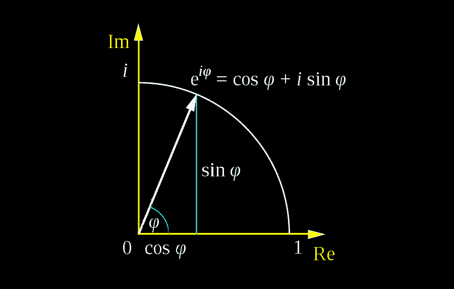
Let us unpack what happens to our sine function as we Laplace-transform it. We begin by noticing that a sine function can be expressed as a
complex exponential
— an indirect result of the celebrated
Euler’s formula
:\[e^{it} = \cos t + i \sin t\]In fact, a sine is often expressed in terms of exponentials for
ease of calculation
, so if we apply that to the function $f(t) = \sin (at)$, we would get: \[ \sin(at) = \frac{e^{iat}-e^{-iat}}{2i} \]Thus the
Laplace transform
of $\sin(at)$ then becomes:
\[ \mathcal{L}\{\sin(at)\} = \frac{1}{2i} \int\limits_0^{\infty} (e^{iat}-e^{-iat}) e^{-st} \, dt \]which means that we have a
product of exponentials
. Distributing the terms, we get:
\[ \mathcal{L}\{\sin(at)\} = \frac{1}{2i} \int\limits_0^{\infty} e^{iat-st}-e^{-iat-st} \, dt \]
Here,
factoring
the $t$ in the exponents yields:
\[ \mathcal{L}\{\sin(at)\} = \frac{1}{2i} \int\limits_0^{\infty} e^{(ia-s)t}-e^{(-ia-s)t} \, dt \]and since $\mathrm{Re}(s) \gt 0$ by assumption, we can proceed with the integration from $0$ to $\infty$ as usual:
\[ \mathcal{L}\{\sin(at)\} = \left.\frac{e^{(ia-s)t}}{2i (ia-s)}\right|_0^{\infty}-\left.\frac{e^{(-ia-s)t}}{2i (-ia-s)}\right|_0^{\infty} \]
Let us simplify further.
Distributing
the $i$ inside the parentheses, we get:
\[ \mathcal{L}\{\sin(at)\} = \left.\frac{e^{(ia-s)t}}{2(-a-is)}\right|_0^{\infty}-\left.\frac{e^{(-ia-s)t}}{2(a-is)}\right|_0^{\infty} \]By evaluating the $t$ at the
boundaries
, we get:
\[ \mathcal{L}\{\sin(at)\} = \left( \frac{e^{(ia-s) \cdot \infty}}{2(-a-is)}-\frac{e^{(ia-s) \cdot 0}}{2 (-a-is)}\right)-\left(\frac{e^{(-ia-s)\cdot\infty}}{2(a-is)}-\frac{e^{(-ia-s)\cdot 0}}{2(a-is)}\right) \]And because $\mathrm{Re}(s) > 0$ by assumption, both $e^{(ia-s) \cdot \infty}$ and $e^{(-ia-s)\cdot\infty}$ oscillate to $0$ (i.e.,
vanish at infinity
), after which we are then left with:\[ \mathcal{L}\{\sin(at)\} = \frac{1}{-2(-a-is)} + \frac{1}{2(a-is)} \]Once there, merging the
fractions
together would yield:\begin{align*} \mathcal{L}\{\sin(at)\} & = \frac{2(a-is)-2(-a-is)}{-4 (a-is)(-a-is)} \\ & = \frac{2a-2is + 2a+2is}{4 (a^2 + isa-isa + s^2)} \\ & = \frac{4a}{4(a^2 + s^2)} \\ & = \frac{a}{a^2 + s^2} \end{align*}which shows that after Laplace transform, a sine is turned into a more tractable
geometric function
. By following similar reasoning, the Laplace transform of cosine can be shown to be equal to the following expression as well: \[ \mathcal{L}\{\cos (at)\} = \frac{s}{a^2 + s^2} \qquad (\mathrm{Re}(s) > 0) \] But then, one might argue “Why do we need to transform trigonometric functions like this when we can just
integrate
them?”
Diverging Functions: What the Laplace Transform is for
What if we throw a wrench in there by introducing a
diverging function
, say, $f(t)=e^{at}$? As it turns out, the Laplace transform of the exponential $e^{at}$ is actually deceptively simple: \begin{align*} \mathcal{L}\{e^{at}\} & = \int_0^{\infty} e^{at}e^{-st} \, dt \\ & = \int_0^{\infty} e^{(a-s)t} \, dt \end{align*}Here, we see that so long as $\mathrm{Re}(s) \gt a$, we would get that: \begin{align*} \int_0^{\infty} e^{(a-s)t} \, dt & = \left. \frac{e^{(a-s)t}}{a-s} \right|_0^{\infty} \\ & = 0-\frac{1}{a-s} \\ & = \frac{1}{s-a} \end{align*} That is, as long as $\mathrm{Re}(s) > a$, the Laplace transform of $e^{at}$ is a simple $1/(s-a)$. Here’s a
video version
of the derivation for the record.
On the other hand, if we mix the exponential $e^{at}$ with the
power function
$t^n$, we would then have: \[ \mathcal{L}\{t^n e^{at}\} = \int\limits_0^{\infty} t^n e^{at} e^{-st} \, dt \] which, after a bit of
recursion
and
integration by parts
, would become:\[ \frac{n!}{(s-a)^{n+1}} \]Here, notice how the transforms of exponential and power function are both
represented
in the expression, with the factorial $n!$, the $1/(s-a)$ fraction, and the $n + 1$ exponent.
In fact, it turns out that we can integrate
any
function with the Laplace transform, as long as it does not
diverge
faster than the $e^{at}$ exponential. In the tables of Laplace transforms, you might have noticed the $\mathrm{Re}(s) \gt a$ condition. That is what the condition is alluding to.
A Transform of Unfathomable Power
However, what we have seen is only the tip of the iceberg, since we can also use Laplace transform to transform the
derivatives
as well. In goes $f^{(n)}(t)$. Something happens. Then out goes:\[ s^n \mathcal{L}\{f(t)\}-\sum_{r=0}^{n-1} s^{n-1-r} f^{(r)}(0) \]For example, when $n=2$, we have that:\[ \mathcal{L}\{f^{\prime\prime}(t)\} = s^2 \mathcal{L}\{f(t)\}-sf(0)-f'(0) \]In addition to the derivatives, the $\mathcal{L}$ can also process some
integrals
: the integral sine, cosine and exponential, as well as the
error function
— to name a few.
But that’s not all. There is also the
inverse Laplace transform
, which takes a frequency-domain function and renders a time-domain function.
In fact, performing the transform from time to frequency and back once introduces a factor of $1/2\pi$. Sometimes, you’ll see the whole fraction in front of the inverse function, while other times, the transform and its inverse share a factor of $1/\sqrt{2\pi}$.
This is as if the Kraken could restitute the boat intact — but only for a factor of $1/2\pi$.
The Laplace transform, even after all those years, never ceases to bring us awe with its power. Here’s a
table
summarizing the transforms we’ve discussed thus far:
Function
Laplace Transform
$1$
$\dfrac{1}{s}$
$t$
$\dfrac{1}{s^2}$
$t^n$
$\dfrac{n!}{s^{n+1}}$
$e^{at}$
$\dfrac{1}{s-a}$
$\sin(at)$
$\dfrac{a}{a^2+s^2}$
$\cos(at)$
$\dfrac{s}{a^2+s^2}$
$t^n e^{at}$
$\dfrac{n!}{(s-a)^{n+1}}$
$f^{(2)}(t)$
$\displaystyle s^2 \mathcal{L}\{f(t)\}-sf(0)-f'(0)$
$f^{(n)}(t)$
$\displaystyle s^n \mathcal{L}\{f(t)\}-\sum_{r=0}^{n-1} s^{n-1-r} f^{(r)}(0)$ | ||||||||||||
| Markdown | 
[](https://mathvault.ca/)
- [Learn](https://mathvault.ca/laplace-transform/)
- [Hub](https://mathvault.ca/hub/)
Definitive resource hub on everything higher math
- [Vault](https://mathvault.ca/vault/)
Bonus guides and lessons on mathematics and other related topics
- [Products & Services](https://mathvault.ca/shop)
- [Definitive Guide to Learning Higher Mathematics](https://mathvault.ca/higher-math-learning-guide/)
- [Ultimate LaTeX Reference Guide](https://mathvault.ca/latex/)
- [Comprehensive List of Mathematical Symbols](https://mathvault.ca/product/comprehensive-list-of-mathematical-symbols/)
- [Math Tutoring / Consulting](https://mathvault.ca/tutoring/)
- [Resources]()
- [Higher Math Proficiency Test](https://mathvault.ca/math-test/)
- [10 Commandments of Higher Math Learning](https://mathvault.ca/10-commandments/)
- [Math Vault Linear Algebra Ebook Series](https://mathvault.ca/free-ebooks-series/)
- [Recommended Math Books](https://mathvault.ca/books/)
- [Recommended Math Websites](https://mathvault.ca/websites/)
- [Recommended Online Tools](https://mathvault.ca/online-tools/)
- [About]()
- [About Us](https://mathvault.ca/about/)
Where we came from, and where we're going
- [Write for Us](https://mathvault.ca/write-for-us/)
Join us in contributing to the glory of mathematics
[Start Here](https://mathvault.ca/introduction-series/)
[Kim Thibault](https://mathvault.ca/author/kimthibo/ "Kim Thibault")
# Laplace Transform: A First Introduction
College Math, Calculus, Complex Number
- [Home](https://mathvault.ca/)
- »
- [Vault](https://mathvault.ca/vault/)
- »
- [College Math](https://mathvault.ca/college-math/)
- »
- Laplace Transform: A First Introduction
Let us take a moment to ponder how truly bizarre the **[Laplace transform](https://mathvault.ca/hub/higher-math/math-symbols/calculus-analysis-symbols/#Key_Transforms)** is.
You put in a sine and get an oddly simple, **arbitrary-looking fraction**. Why do we suddenly have squares?
You look at the table of **common Laplace transforms** to find a pattern and you see no rhyme, no reason, no obvious link between different functions and their different, very different, results.
What’s going on here?
Or so we thought when we first encountered the cursive \$\\mathcal{L}\$ in school.
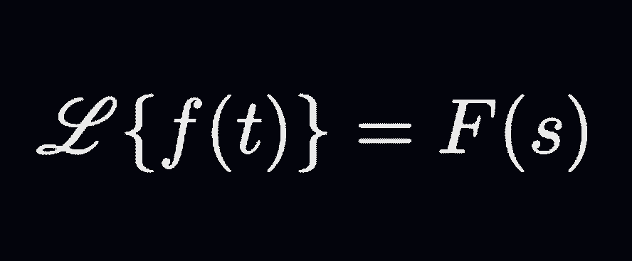
Table of Contents
[Toggle](https://mathvault.ca/laplace-transform/)
- [What does the Laplace transform do, really?](https://mathvault.ca/laplace-transform/#What_does_the_Laplace_transform_do_really)
- [Some Preliminary Examples](https://mathvault.ca/laplace-transform/#Some_Preliminary_Examples)
- [Looking Inside the Laplace Transform of Sine](https://mathvault.ca/laplace-transform/#Looking_Inside_the_Laplace_Transform_of_Sine)
- [Diverging Functions: What the Laplace Transform is for](https://mathvault.ca/laplace-transform/#Diverging_Functions_What_the_Laplace_Transform_is_for)
- [A Transform of Unfathomable Power](https://mathvault.ca/laplace-transform/#A_Transform_of_Unfathomable_Power)
## [What does the Laplace transform do, really?](https://mathvault.ca/laplace-transform/#toc)
At a high level, Laplace transform is an **[integral transform](https://en.wikipedia.org/wiki/Integral_transform#:~:text=In%20mathematics%2C%20an%20integral%20transform,in%20the%20original%20function%20space.)** mostly encountered in differential equations — in electrical engineering for instance — where electric circuits are represented as differential equations.
In fact, it takes a **time-domain function**, where \$t\$ is the variable, and outputs a **frequency-domain function**, where \$s\$ is the variable. Definition-wise, Laplace transform takes a function of real variable \$f(t)\$ (defined for all \$t \\ge 0\$) to a function of complex variable \$F(s)\$ as follows:
\\\[\\mathcal{L}\\{f(t)\\} = \\int\_0^{\\infty} f(t) e^{-st} \\, dt = F(s) \\\]
## [Some Preliminary Examples](https://mathvault.ca/laplace-transform/#toc)
What fate awaits **simple functions** as they enter the Laplace transform?
Take the simplest function: the **constant function** \$f(t)=1\$. In this case, putting \$1\$ in the transform yields \$1/s\$, which means that we went from a constant to a variable-dependent function.
(Odd but not too worrying. After all, we’ve seen \$1/x\$ integrating to \$\\ln x\$ in calculus. Not a constant-to-variable situation of course, but an unexpected transformation nonetheless.)
Let us take it up a notch, with the **linear function** \$f(t) = t\$. After the transformation, it is turned into \$1/s^2\$, which means that we went from \$1 \\to 1/s\$ to \$t \\to 1/s^2\$. A pattern begins to emerge.
Now what about \$f(t)=t^n\$? With this simple **power function**, we end up with: \\\[ \\mathcal{L}\\{ t^n \\} = \\frac{n!}{s^{n+1}}\\\] So there was a factorial in \$\\mathcal{L}\\{t\\}\$ all along, hidden by the fact that \$1! = 1\$. What else is the transform hiding?
Here, a glance at a table of **[common Laplace transforms](https://tutorial.math.lamar.edu/pdf/Laplace_Table.pdf)** would show that the emerging pattern cannot explain other functions easily. Things get weird, and the weirdness escalates quickly — which brings us back to the sine function.
## [Looking Inside the Laplace Transform of Sine](https://mathvault.ca/laplace-transform/#toc)
Let us unpack what happens to our sine function as we Laplace-transform it. We begin by noticing that a sine function can be expressed as a **complex exponential** — an indirect result of the celebrated [Euler’s formula](https://mathvault.ca/euler-formula/):\\\[e^{it} = \\cos t + i \\sin t\\\]In fact, a sine is often expressed in terms of exponentials for **ease of calculation**, so if we apply that to the function \$f(t) = \\sin (at)\$, we would get: \\\[ \\sin(at) = \\frac{e^{iat}-e^{-iat}}{2i} \\\]Thus the **Laplace transform** of \$\\sin(at)\$ then becomes:
\\\[ \\mathcal{L}\\{\\sin(at)\\} = \\frac{1}{2i} \\int\\limits\_0^{\\infty} (e^{iat}-e^{-iat}) e^{-st} \\, dt \\\]which means that we have a **product of exponentials**. Distributing the terms, we get:
\\\[ \\mathcal{L}\\{\\sin(at)\\} = \\frac{1}{2i} \\int\\limits\_0^{\\infty} e^{iat-st}-e^{-iat-st} \\, dt \\\]
Here, **factoring** the \$t\$ in the exponents yields:
\\\[ \\mathcal{L}\\{\\sin(at)\\} = \\frac{1}{2i} \\int\\limits\_0^{\\infty} e^{(ia-s)t}-e^{(-ia-s)t} \\, dt \\\]and since \$\\mathrm{Re}(s) \\gt 0\$ by assumption, we can proceed with the integration from \$0\$ to \$\\infty\$ as usual:
\\\[ \\mathcal{L}\\{\\sin(at)\\} = \\left.\\frac{e^{(ia-s)t}}{2i (ia-s)}\\right\|\_0^{\\infty}-\\left.\\frac{e^{(-ia-s)t}}{2i (-ia-s)}\\right\|\_0^{\\infty} \\\]
Let us simplify further. **Distributing** the \$i\$ inside the parentheses, we get:
\\\[ \\mathcal{L}\\{\\sin(at)\\} = \\left.\\frac{e^{(ia-s)t}}{2(-a-is)}\\right\|\_0^{\\infty}-\\left.\\frac{e^{(-ia-s)t}}{2(a-is)}\\right\|\_0^{\\infty} \\\]By evaluating the \$t\$ at the **boundaries**, we get:
\\\[ \\mathcal{L}\\{\\sin(at)\\} = \\left( \\frac{e^{(ia-s) \\cdot \\infty}}{2(-a-is)}-\\frac{e^{(ia-s) \\cdot 0}}{2 (-a-is)}\\right)-\\left(\\frac{e^{(-ia-s)\\cdot\\infty}}{2(a-is)}-\\frac{e^{(-ia-s)\\cdot 0}}{2(a-is)}\\right) \\\]And because \$\\mathrm{Re}(s) \> 0\$ by assumption, both \$e^{(ia-s) \\cdot \\infty}\$ and \$e^{(-ia-s)\\cdot\\infty}\$ oscillate to \$0\$ (i.e., **[vanish at infinity](https://mathvault.ca/math-glossary/#vanish)**), after which we are then left with:\\\[ \\mathcal{L}\\{\\sin(at)\\} = \\frac{1}{-2(-a-is)} + \\frac{1}{2(a-is)} \\\]Once there, merging the **fractions** together would yield:\\begin{align\*} \\mathcal{L}\\{\\sin(at)\\} & = \\frac{2(a-is)-2(-a-is)}{-4 (a-is)(-a-is)} \\\\ & = \\frac{2a-2is + 2a+2is}{4 (a^2 + isa-isa + s^2)} \\\\ & = \\frac{4a}{4(a^2 + s^2)} \\\\ & = \\frac{a}{a^2 + s^2} \\end{align\*}which shows that after Laplace transform, a sine is turned into a more tractable **geometric function**. By following similar reasoning, the Laplace transform of cosine can be shown to be equal to the following expression as well: \\\[ \\mathcal{L}\\{\\cos (at)\\} = \\frac{s}{a^2 + s^2} \\qquad (\\mathrm{Re}(s) \> 0) \\\] But then, one might argue “Why do we need to transform trigonometric functions like this when we can just **integrate** them?”
## [Diverging Functions: What the Laplace Transform is for](https://mathvault.ca/laplace-transform/#toc)
What if we throw a wrench in there by introducing a **diverging function**, say, \$f(t)=e^{at}\$? As it turns out, the Laplace transform of the exponential \$e^{at}\$ is actually deceptively simple: \\begin{align\*} \\mathcal{L}\\{e^{at}\\} & = \\int\_0^{\\infty} e^{at}e^{-st} \\, dt \\\\ & = \\int\_0^{\\infty} e^{(a-s)t} \\, dt \\end{align\*}Here, we see that so long as \$\\mathrm{Re}(s) \\gt a\$, we would get that: \\begin{align\*} \\int\_0^{\\infty} e^{(a-s)t} \\, dt & = \\left. \\frac{e^{(a-s)t}}{a-s} \\right\|\_0^{\\infty} \\\\ & = 0-\\frac{1}{a-s} \\\\ & = \\frac{1}{s-a} \\end{align\*} That is, as long as \$\\mathrm{Re}(s) \> a\$, the Laplace transform of \$e^{at}\$ is a simple \$1/(s-a)\$. Here’s a **video version** of the derivation for the record.
On the other hand, if we mix the exponential \$e^{at}\$ with the **power function** \$t^n\$, we would then have: \\\[ \\mathcal{L}\\{t^n e^{at}\\} = \\int\\limits\_0^{\\infty} t^n e^{at} e^{-st} \\, dt \\\] which, after a bit of [recursion](https://mathvault.ca/math-glossary/#recursion) and [integration by parts](https://mathvault.ca/integration-overshooting-method/#Integration_By_Parts), would become:\\\[ \\frac{n!}{(s-a)^{n+1}} \\\]Here, notice how the transforms of exponential and power function are both **represented** in the expression, with the factorial \$n!\$, the \$1/(s-a)\$ fraction, and the \$n + 1\$ exponent.
In fact, it turns out that we can integrate *any* function with the Laplace transform, as long as it does not **diverge** faster than the \$e^{at}\$ exponential. In the tables of Laplace transforms, you might have noticed the \$\\mathrm{Re}(s) \\gt a\$ condition. That is what the condition is alluding to.
## [A Transform of Unfathomable Power](https://mathvault.ca/laplace-transform/#toc)
However, what we have seen is only the tip of the iceberg, since we can also use Laplace transform to transform the **derivatives** as well. In goes \$f^{(n)}(t)\$. Something happens. Then out goes:\\\[ s^n \\mathcal{L}\\{f(t)\\}-\\sum\_{r=0}^{n-1} s^{n-1-r} f^{(r)}(0) \\\]For example, when \$n=2\$, we have that:\\\[ \\mathcal{L}\\{f^{\\prime\\prime}(t)\\} = s^2 \\mathcal{L}\\{f(t)\\}-sf(0)-f'(0) \\\]In addition to the derivatives, the \$\\mathcal{L}\$ can also process some **integrals**: the integral sine, cosine and exponential, as well as the [error function](https://mathvault.ca/hub/higher-math/math-symbols/probability-statistics-symbols/#Continuous_Probability_Distributions_and_Associated_Functions) — to name a few.
But that’s not all. There is also the **[inverse Laplace transform](https://mathvault.ca/hub/higher-math/math-symbols/calculus-analysis-symbols/#Key_Transforms)**, which takes a frequency-domain function and renders a time-domain function.
In fact, performing the transform from time to frequency and back once introduces a factor of \$1/2\\pi\$. Sometimes, you’ll see the whole fraction in front of the inverse function, while other times, the transform and its inverse share a factor of \$1/\\sqrt{2\\pi}\$.
This is as if the Kraken could restitute the boat intact — but only for a factor of \$1/2\\pi\$.
The Laplace transform, even after all those years, never ceases to bring us awe with its power. Here’s a **table** summarizing the transforms we’ve discussed thus far:
| Function | Laplace Transform |
|---|---|
| \$1\$ | \$\\dfrac{1}{s}\$ |
| \$t\$ | \$\\dfrac{1}{s^2}\$ |
| \$t^n\$ | \$\\dfrac{n!}{s^{n+1}}\$ |
| \$e^{at}\$ | \$\\dfrac{1}{s-a}\$ |
| \$\\sin(at)\$ | \$\\dfrac{a}{a^2+s^2}\$ |
| \$\\cos(at)\$ | \$\\dfrac{s}{a^2+s^2}\$ |
| \$t^n e^{at}\$ | \$\\dfrac{n!}{(s-a)^{n+1}}\$ |
| \$f^{(2)}(t)\$ | \$\\displaystyle s^2 \\mathcal{L}\\{f(t)\\}-sf(0)-f'(0)\$ |
| \$f^{(n)}(t)\$ | \$\\displaystyle s^n \\mathcal{L}\\{f(t)\\}-\\sum\_{r=0}^{n-1} s^{n-1-r} f^{(r)}(0)\$ |
[](https://mathvault.ca/higher-math-learning-guide/)
How's your higher math going?
Shallow learning and mechanical practices rarely work in higher mathematics. Instead, use these 10 principles to **optimize your learning** and prevent years of wasted effort.
[Hmm... **Tell me more.**](https://mathvault.ca/higher-math-learning-guide/)
- 100shares

Kim Thibault
#### About the author
Kim Thibault is an incorrigible polymath. After a Ph.D. in Physics, she did applied research in machine learning for audio, then a stint in programming, to finally become an author and scientific translator. She occasionally solves differential equations as a hobby. Find her on her [**website**](http://kimthibault.com/) and on [**Linkedin**](https://linkedin.com/in/kimthibaultphd).
[« Previous PostThe Definitive Glossary of Higher Mathematical Jargon](https://mathvault.ca/math-glossary/)
[Next Post »Euler’s Formula: A Complete Guide](https://mathvault.ca/euler-formula/)
#### You may also like
[](https://mathvault.ca/euler-formula/ "Euler’s Formula: A Complete Guide")
Euler’s Formula: A Complete Guide
[Euler’s Formula: A Complete Guide](https://mathvault.ca/euler-formula/)
[](https://mathvault.ca/statistical-significance/ "A First Introduction to Statistical Significance — Through Dice Rolling and Other Uncanny Examples")
A First Introduction to Statistical Significance — Through Dice Rolling and Other Uncanny Examples
[A First Introduction to Statistical Significance — Through Dice Rolling and Other Uncanny Examples](https://mathvault.ca/statistical-significance/)
#### Leave a Reply
[Cancel reply](https://mathvault.ca/laplace-transform/#respond)
1. 
**Precious Amadi** says:
[February 10, 2021 at 2:11 AM](https://mathvault.ca/laplace-transform/#comment-3586)
Any link to download soft copy?
[Reply](https://mathvault.ca/laplace-transform/#comment-3586)
1. [](https://mathvault.ca/) **[Math Vault](https://mathvault.ca/)** says:
[February 10, 2021 at 2:02 PM](https://mathvault.ca/laplace-transform/#comment-3587)
Hi Amadi. Thanks for your interest. If you click on the “Print” button in your browser, you can save the guide as a PDF. That would be a way of generating a soft copy.
[Reply](https://mathvault.ca/laplace-transform/#comment-3587)
{"email":"Email address invalid","url":"Website address invalid","required":"Required field missing"}
#### Search
***
#### Navigational Menu
***
[**General** **M****a****th**](https://mathvault.ca/general-math/)
[**Alg****e****bra**](https://mathvault.ca/general-math/algebra/)
[**Func****tions &** **Operations**](https://mathvault.ca/general-math/functions-operations/)
[**College** **M****ath**](https://mathvault.ca/college-math)
[**Calc****ul****us**](https://mathvault.ca/college-math/calculus/)
[**Probab****ilit****y & Statistics**](https://mathvault.ca/college-math/probability-statistics/)
[**Foundation** **o****f Higher Math**](https://mathvault.ca/foundation-of-higher-math/)
[**Math** **Too****ls**](https://mathvault.ca/math-tools/)
#### Useful Resources
***
[Higher Math Exploration Series](https://mathvault.ca/introduction-series/)
[10 Commandments of Higher Math Learning](https://mathvault.ca/10-commandments/)
[Compendium of Math Symbols](https://mathvault.ca/hub/higher-math/math-symbols)
[Higher Math Proficiency Test](https://mathvault.ca/math-test/)
#### Math eBooks
***
[Definitive Guide to Learning Higher Math](https://mathvault.ca/higher-math-learning-guide/)
[Ultimate LaTeX Reference Guide](https://mathvault.ca/latex/)
[Linear Algebra eBook Series](https://mathvault.ca/free-ebooks-series/)
#### Popular Guides
***
## [The Definitive Glossary of Higher Mathematical Jargon](https://mathvault.ca/math-glossary/ "The Definitive Glossary of Higher Mathematical Jargon")
[The Definitive Glossary of Higher Mathematical Jargon](https://mathvault.ca/math-glossary/)
## [The Definitive, Non-Technical Introduction to LaTeX, Professional Typesetting and Scientific Publishing](https://mathvault.ca/latex-guide/ "The Definitive, Non-Technical Introduction to LaTeX, Professional Typesetting and Scientific Publishing")
[The Definitive, Non-Technical Introduction to LaTeX, Professional Typesetting and Scientific Publishing](https://mathvault.ca/latex-guide/)
## [The Definitive Higher Math Guide on Integer Long Division (and Its Variants)](https://mathvault.ca/long-division/ "The Definitive Higher Math Guide on Integer Long Division (and Its Variants)")
[The Definitive Higher Math Guide on Integer Long Division (and Its Variants)](https://mathvault.ca/long-division/)
About Math Vault
Originally founded as a Montreal-based math tutoring agency, Math Vault has since then morphed into a global resource hub for people interested in learning more about higher mathematics. For more, see [about us](https://mathvault.ca/about/).
Guides
[Definitive Guide to Learning Higher Math](https://mathvault.ca/higher-math-learning-guide/)
[Ultimate LaTeX Reference Guide](https://mathvault.ca/latex/)
[Comprehensive List of Math Symbols](https://mathvault.ca/product/comprehensive-list-of-mathematical-symbols/)
[Linear Algebra eBook Series](https://mathvault.ca/free-ebooks-series/)
Resources & Tools
[Higher Math Exploration Series](https://mathvault.ca/introduction-series/)
[Higher Math Proficiency Test](https://mathvault.ca/math-test/)
[10 Commandments of Higher Math Learning](https://mathvault.ca/10-commandments/)
Contact
[About Us](https://mathvault.ca/about/)
[Write for Us](https://mathvault.ca/write-for-us/)
© 2026 Math Vault. All Rights Reserved.
[Privacy Policy](https://mathvault.ca/privacy-policy/) [Terms of Use](https://mathvault.ca/terms-of-use/) [Anti-Spam](https://mathvault.ca/anti-spam-policy/) [Disclosure](https://mathvault.ca/affiliate-disclosure/) [DMCA Notice](https://mathvault.ca/dmca/)
- 100shares
[Math Vault](https://mathvault.ca/?blackhole=04423849df "Do NOT follow this link or you will be banned from the site!") | ||||||||||||
| Readable Markdown | Let us take a moment to ponder how truly bizarre the **[Laplace transform](https://mathvault.ca/hub/higher-math/math-symbols/calculus-analysis-symbols/#Key_Transforms)** is.
You put in a sine and get an oddly simple, **arbitrary-looking fraction**. Why do we suddenly have squares?
You look at the table of **common Laplace transforms** to find a pattern and you see no rhyme, no reason, no obvious link between different functions and their different, very different, results.
What’s going on here?
Or so we thought when we first encountered the cursive \$\\mathcal{L}\$ in school.

Table of Contents
- [What does the Laplace transform do, really?](https://mathvault.ca/laplace-transform/#What_does_the_Laplace_transform_do_really)
- [Some Preliminary Examples](https://mathvault.ca/laplace-transform/#Some_Preliminary_Examples)
- [Looking Inside the Laplace Transform of Sine](https://mathvault.ca/laplace-transform/#Looking_Inside_the_Laplace_Transform_of_Sine)
- [Diverging Functions: What the Laplace Transform is for](https://mathvault.ca/laplace-transform/#Diverging_Functions_What_the_Laplace_Transform_is_for)
- [A Transform of Unfathomable Power](https://mathvault.ca/laplace-transform/#A_Transform_of_Unfathomable_Power)
## [What does the Laplace transform do, really?](https://mathvault.ca/laplace-transform/#toc)
At a high level, Laplace transform is an **[integral transform](https://en.wikipedia.org/wiki/Integral_transform#:~:text=In%20mathematics%2C%20an%20integral%20transform,in%20the%20original%20function%20space.)** mostly encountered in differential equations — in electrical engineering for instance — where electric circuits are represented as differential equations.
In fact, it takes a **time-domain function**, where \$t\$ is the variable, and outputs a **frequency-domain function**, where \$s\$ is the variable. Definition-wise, Laplace transform takes a function of real variable \$f(t)\$ (defined for all \$t \\ge 0\$) to a function of complex variable \$F(s)\$ as follows:
\\\[\\mathcal{L}\\{f(t)\\} = \\int\_0^{\\infty} f(t) e^{-st} \\, dt = F(s) \\\]
## [Some Preliminary Examples](https://mathvault.ca/laplace-transform/#toc)
What fate awaits **simple functions** as they enter the Laplace transform?
Take the simplest function: the **constant function** \$f(t)=1\$. In this case, putting \$1\$ in the transform yields \$1/s\$, which means that we went from a constant to a variable-dependent function.
(Odd but not too worrying. After all, we’ve seen \$1/x\$ integrating to \$\\ln x\$ in calculus. Not a constant-to-variable situation of course, but an unexpected transformation nonetheless.)
Let us take it up a notch, with the **linear function** \$f(t) = t\$. After the transformation, it is turned into \$1/s^2\$, which means that we went from \$1 \\to 1/s\$ to \$t \\to 1/s^2\$. A pattern begins to emerge.
Now what about \$f(t)=t^n\$? With this simple **power function**, we end up with: \\\[ \\mathcal{L}\\{ t^n \\} = \\frac{n!}{s^{n+1}}\\\] So there was a factorial in \$\\mathcal{L}\\{t\\}\$ all along, hidden by the fact that \$1! = 1\$. What else is the transform hiding?
Here, a glance at a table of **[common Laplace transforms](https://tutorial.math.lamar.edu/pdf/Laplace_Table.pdf)** would show that the emerging pattern cannot explain other functions easily. Things get weird, and the weirdness escalates quickly — which brings us back to the sine function.
## [Looking Inside the Laplace Transform of Sine](https://mathvault.ca/laplace-transform/#toc)
Let us unpack what happens to our sine function as we Laplace-transform it. We begin by noticing that a sine function can be expressed as a **complex exponential** — an indirect result of the celebrated [Euler’s formula](https://mathvault.ca/euler-formula/):\\\[e^{it} = \\cos t + i \\sin t\\\]In fact, a sine is often expressed in terms of exponentials for **ease of calculation**, so if we apply that to the function \$f(t) = \\sin (at)\$, we would get: \\\[ \\sin(at) = \\frac{e^{iat}-e^{-iat}}{2i} \\\]Thus the **Laplace transform** of \$\\sin(at)\$ then becomes:
\\\[ \\mathcal{L}\\{\\sin(at)\\} = \\frac{1}{2i} \\int\\limits\_0^{\\infty} (e^{iat}-e^{-iat}) e^{-st} \\, dt \\\]which means that we have a **product of exponentials**. Distributing the terms, we get:
\\\[ \\mathcal{L}\\{\\sin(at)\\} = \\frac{1}{2i} \\int\\limits\_0^{\\infty} e^{iat-st}-e^{-iat-st} \\, dt \\\]
Here, **factoring** the \$t\$ in the exponents yields:
\\\[ \\mathcal{L}\\{\\sin(at)\\} = \\frac{1}{2i} \\int\\limits\_0^{\\infty} e^{(ia-s)t}-e^{(-ia-s)t} \\, dt \\\]and since \$\\mathrm{Re}(s) \\gt 0\$ by assumption, we can proceed with the integration from \$0\$ to \$\\infty\$ as usual:
\\\[ \\mathcal{L}\\{\\sin(at)\\} = \\left.\\frac{e^{(ia-s)t}}{2i (ia-s)}\\right\|\_0^{\\infty}-\\left.\\frac{e^{(-ia-s)t}}{2i (-ia-s)}\\right\|\_0^{\\infty} \\\]
Let us simplify further. **Distributing** the \$i\$ inside the parentheses, we get:
\\\[ \\mathcal{L}\\{\\sin(at)\\} = \\left.\\frac{e^{(ia-s)t}}{2(-a-is)}\\right\|\_0^{\\infty}-\\left.\\frac{e^{(-ia-s)t}}{2(a-is)}\\right\|\_0^{\\infty} \\\]By evaluating the \$t\$ at the **boundaries**, we get:
\\\[ \\mathcal{L}\\{\\sin(at)\\} = \\left( \\frac{e^{(ia-s) \\cdot \\infty}}{2(-a-is)}-\\frac{e^{(ia-s) \\cdot 0}}{2 (-a-is)}\\right)-\\left(\\frac{e^{(-ia-s)\\cdot\\infty}}{2(a-is)}-\\frac{e^{(-ia-s)\\cdot 0}}{2(a-is)}\\right) \\\]And because \$\\mathrm{Re}(s) \> 0\$ by assumption, both \$e^{(ia-s) \\cdot \\infty}\$ and \$e^{(-ia-s)\\cdot\\infty}\$ oscillate to \$0\$ (i.e., **[vanish at infinity](https://mathvault.ca/math-glossary/#vanish)**), after which we are then left with:\\\[ \\mathcal{L}\\{\\sin(at)\\} = \\frac{1}{-2(-a-is)} + \\frac{1}{2(a-is)} \\\]Once there, merging the **fractions** together would yield:\\begin{align\*} \\mathcal{L}\\{\\sin(at)\\} & = \\frac{2(a-is)-2(-a-is)}{-4 (a-is)(-a-is)} \\\\ & = \\frac{2a-2is + 2a+2is}{4 (a^2 + isa-isa + s^2)} \\\\ & = \\frac{4a}{4(a^2 + s^2)} \\\\ & = \\frac{a}{a^2 + s^2} \\end{align\*}which shows that after Laplace transform, a sine is turned into a more tractable **geometric function**. By following similar reasoning, the Laplace transform of cosine can be shown to be equal to the following expression as well: \\\[ \\mathcal{L}\\{\\cos (at)\\} = \\frac{s}{a^2 + s^2} \\qquad (\\mathrm{Re}(s) \> 0) \\\] But then, one might argue “Why do we need to transform trigonometric functions like this when we can just **integrate** them?”
## [Diverging Functions: What the Laplace Transform is for](https://mathvault.ca/laplace-transform/#toc)
What if we throw a wrench in there by introducing a **diverging function**, say, \$f(t)=e^{at}\$? As it turns out, the Laplace transform of the exponential \$e^{at}\$ is actually deceptively simple: \\begin{align\*} \\mathcal{L}\\{e^{at}\\} & = \\int\_0^{\\infty} e^{at}e^{-st} \\, dt \\\\ & = \\int\_0^{\\infty} e^{(a-s)t} \\, dt \\end{align\*}Here, we see that so long as \$\\mathrm{Re}(s) \\gt a\$, we would get that: \\begin{align\*} \\int\_0^{\\infty} e^{(a-s)t} \\, dt & = \\left. \\frac{e^{(a-s)t}}{a-s} \\right\|\_0^{\\infty} \\\\ & = 0-\\frac{1}{a-s} \\\\ & = \\frac{1}{s-a} \\end{align\*} That is, as long as \$\\mathrm{Re}(s) \> a\$, the Laplace transform of \$e^{at}\$ is a simple \$1/(s-a)\$. Here’s a **video version** of the derivation for the record.
On the other hand, if we mix the exponential \$e^{at}\$ with the **power function** \$t^n\$, we would then have: \\\[ \\mathcal{L}\\{t^n e^{at}\\} = \\int\\limits\_0^{\\infty} t^n e^{at} e^{-st} \\, dt \\\] which, after a bit of [recursion](https://mathvault.ca/math-glossary/#recursion) and [integration by parts](https://mathvault.ca/integration-overshooting-method/#Integration_By_Parts), would become:\\\[ \\frac{n!}{(s-a)^{n+1}} \\\]Here, notice how the transforms of exponential and power function are both **represented** in the expression, with the factorial \$n!\$, the \$1/(s-a)\$ fraction, and the \$n + 1\$ exponent.
In fact, it turns out that we can integrate *any* function with the Laplace transform, as long as it does not **diverge** faster than the \$e^{at}\$ exponential. In the tables of Laplace transforms, you might have noticed the \$\\mathrm{Re}(s) \\gt a\$ condition. That is what the condition is alluding to.
## [A Transform of Unfathomable Power](https://mathvault.ca/laplace-transform/#toc)
However, what we have seen is only the tip of the iceberg, since we can also use Laplace transform to transform the **derivatives** as well. In goes \$f^{(n)}(t)\$. Something happens. Then out goes:\\\[ s^n \\mathcal{L}\\{f(t)\\}-\\sum\_{r=0}^{n-1} s^{n-1-r} f^{(r)}(0) \\\]For example, when \$n=2\$, we have that:\\\[ \\mathcal{L}\\{f^{\\prime\\prime}(t)\\} = s^2 \\mathcal{L}\\{f(t)\\}-sf(0)-f'(0) \\\]In addition to the derivatives, the \$\\mathcal{L}\$ can also process some **integrals**: the integral sine, cosine and exponential, as well as the [error function](https://mathvault.ca/hub/higher-math/math-symbols/probability-statistics-symbols/#Continuous_Probability_Distributions_and_Associated_Functions) — to name a few.
But that’s not all. There is also the **[inverse Laplace transform](https://mathvault.ca/hub/higher-math/math-symbols/calculus-analysis-symbols/#Key_Transforms)**, which takes a frequency-domain function and renders a time-domain function.
In fact, performing the transform from time to frequency and back once introduces a factor of \$1/2\\pi\$. Sometimes, you’ll see the whole fraction in front of the inverse function, while other times, the transform and its inverse share a factor of \$1/\\sqrt{2\\pi}\$.
This is as if the Kraken could restitute the boat intact — but only for a factor of \$1/2\\pi\$.
The Laplace transform, even after all those years, never ceases to bring us awe with its power. Here’s a **table** summarizing the transforms we’ve discussed thus far:
| Function | Laplace Transform |
|---|---|
| \$1\$ | \$\\dfrac{1}{s}\$ |
| \$t\$ | \$\\dfrac{1}{s^2}\$ |
| \$t^n\$ | \$\\dfrac{n!}{s^{n+1}}\$ |
| \$e^{at}\$ | \$\\dfrac{1}{s-a}\$ |
| \$\\sin(at)\$ | \$\\dfrac{a}{a^2+s^2}\$ |
| \$\\cos(at)\$ | \$\\dfrac{s}{a^2+s^2}\$ |
| \$t^n e^{at}\$ | \$\\dfrac{n!}{(s-a)^{n+1}}\$ |
| \$f^{(2)}(t)\$ | \$\\displaystyle s^2 \\mathcal{L}\\{f(t)\\}-sf(0)-f'(0)\$ |
| \$f^{(n)}(t)\$ | \$\\displaystyle s^n \\mathcal{L}\\{f(t)\\}-\\sum\_{r=0}^{n-1} s^{n-1-r} f^{(r)}(0)\$ | | ||||||||||||
| ML Classification | |||||||||||||
| ML Categories |
Raw JSON{
"/Science": 837,
"/Science/Mathematics": 827,
"/Science/Mathematics/Other": 804,
"/Computers_and_Electronics": 140
} | ||||||||||||
| ML Page Types |
Raw JSON{
"/Article": 998,
"/Article/Tutorial_or_Guide": 937
} | ||||||||||||
| ML Intent Types |
Raw JSON{
"Informational": 999
} | ||||||||||||
| Content Metadata | |||||||||||||
| Language | en-us | ||||||||||||
| Author | Kim Thibault | ||||||||||||
| Publish Time | 2020-08-08 17:00:00 (5 years ago) | ||||||||||||
| Original Publish Time | 2020-08-08 17:00:00 (5 years ago) | ||||||||||||
| Republished | No | ||||||||||||
| Word Count (Total) | 1,848 | ||||||||||||
| Word Count (Content) | 1,207 | ||||||||||||
| Links | |||||||||||||
| External Links | 14 | ||||||||||||
| Internal Links | 48 | ||||||||||||
| Technical SEO | |||||||||||||
| Meta Nofollow | No | ||||||||||||
| Meta Noarchive | No | ||||||||||||
| JS Rendered | No | ||||||||||||
| Redirect Target | null | ||||||||||||
| Performance | |||||||||||||
| Download Time (ms) | 245 | ||||||||||||
| TTFB (ms) | 223 | ||||||||||||
| Download Size (bytes) | 49,753 | ||||||||||||
| Shard | 120 (laksa) | ||||||||||||
| Root Hash | 8577111680796856520 | ||||||||||||
| Unparsed URL | ca,mathvault!/laplace-transform/ s443 | ||||||||||||