ℹ️ Skipped - page is already crawled
| Filter | Status | Condition | Details |
|---|---|---|---|
| HTTP status | PASS | download_http_code = 200 | HTTP 200 |
| Age cutoff | PASS | download_stamp > now() - 6 MONTH | 1 months ago |
| History drop | PASS | isNull(history_drop_reason) | No drop reason |
| Spam/ban | PASS | fh_dont_index != 1 AND ml_spam_score = 0 | ml_spam_score=0 |
| Canonical | PASS | meta_canonical IS NULL OR = '' OR = src_unparsed | Not set |
| Property | Value |
|---|---|
| URL | https://link.springer.com/article/10.1007/s42081-023-00209-y |
| Last Crawled | 2026-03-24 04:11:39 (28 days ago) |
| First Indexed | 2023-09-20 15:47:31 (2 years ago) |
| HTTP Status Code | 200 |
| Meta Title | Machine learning and the James–Stein estimator | Japanese Journal of Statistics and Data Science | Springer Nature Link |
| Meta Description | It is now 62 years since the publication of James and Stein’s seminal article on the estimation of a multivariate normal mean vector. The paper made |
| Meta Canonical | null |
| Boilerpipe Text | 1
Introduction
By and large, the statistics world is one of heuristics, approximations, and asymptotics. The James–Stein estimator arrived in that world in 1961 on a note of startling specificity: unseen parameters
μ
1
,
μ
2
,
…
,
μ
n
produce independent observations
x
i
∼
ind
N
(
μ
i
,
1
)
,
i
=
1
,
…
,
n
,
(1)
n
≥
3
. The James–Stein rule in its simplest form proposed estimating the
μ
i
by
μ
^
i
J
S
=
(
1
−
n
−
2
S
)
x
i
(
S
=
∑
i
=
1
n
x
i
2
)
.
(2)
Formula (
2
) looked implausible: the estimate of
μ
i
depended on the
other
observations
x
j
,
j
≠
i
(through
S
), as well as
x
i
, despite the independence assumption. Nevertheless, James and Stein showed that Rule (
2
)
always
beat the obvious maximum likelihood estimates
μ
^
i
M
L
=
x
¯
i
(
i
=
1
,
…
,
n
)
(3)
in terms of total expected squared error
E
{
∑
i
=
1
n
(
μ
^
i
−
μ
i
)
2
}
.
(4)
That “always” was the shocking part: two centuries of statistical theory, ANOVA, regression, multivariate analysis, etc., depended on maximum likelihood estimation. Did everything have to be rethought?
One path forward involved Bayesian thinking. If we assumed that the
μ
i
themselves came from a normal distribution,
μ
i
∼
ind
N
(
0
,
A
)
for
i
=
1
,
…
,
n
,
(5)
with variance
A
≥
0
, the Bayes estimates would be
μ
^
i
B
a
y
e
s
=
B
x
i
(
B
=
A
/
(
A
+
1
)
)
.
(6)
We don’t know
A
or
B
but
B
^
=
1
−
(
n
−
2
)
/
S
(7)
is
B
’s unbiased estimate: we can rewrite (
2
) as
μ
^
i
J
S
=
B
^
x
i
,
(8)
which at least looks more plausible.
In the language introduced by Robbins (
1956
), formula (
8
) is an
empirical Bayes
estimator, another shocking post-war statistical innovation. Carl Morris and I wrote a series of papers in the 1970 s exploring Bayesian roots of the James–Stein estimator (Efron and Morris,
1973
). Something is lost in the empirical Bayes formulation, namely the frequentist “always” of expected square error minimization, but a lot is gained in flexibility and scope, as discussed in Sect.
2
.
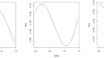
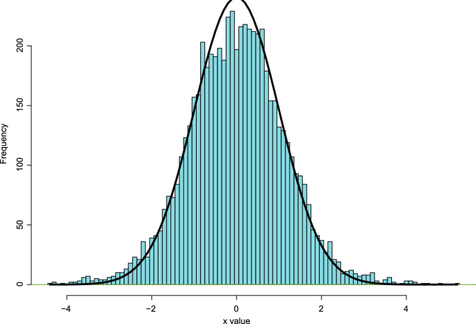
Fig. 1
Prostate data: 6033
x
values; mean 0.003, sd
=
1.135
; curve is proportional to a
N
(
0
,
1
)
density
Full size image
Figure
1
illustrates an example of simultaneous estimation pursued in Sect. 2.1 of Efron (
2010
). A microarray study has compared expression levels between prostate cancer patients and control subjects for
n
=
6033
genes. For each gene, a statistic
x
i
has been calculated (essentially a “
z
-value”),
x
i
∼
N
(
μ
i
,
1
)
,
i
=
1
,
…
,
n
,
(9)
where
μ
i
measures the difference between cancer and control group levels.
The solid curve in Fig.
1
is a
N
(
0
,
1
)
density scaled to have the same area as the histogram of the 6033
x
values. A bad result from the researchers’ point of view would be a perfect fit of curve to histogram, which would imply all the genes have
μ
i
=
0
, the “null” value of no difference between cancer patients and controls.
That’s not what happened: the histogram has mildly heavy tails in both directions. The researchers were hoping to find genes with large values of
‖
μ
i
‖
—ones that might be a clue to prostate cancer etiology—as suggested by the heavy tails. How encouraged should they be?
Not very, according to the James–Stein rule. The 6033
x
i
values have mean 0.003, which I’ll take to be zero, and empirical variance
σ
^
2
=
1.289.
(10)
The James–Stein estimate (
2
) is
μ
^
i
J
S
=
(
1
−
n
−
2
n
−
1
1
σ
^
2
)
x
i
=
0.224
⋅
x
i
,
(11)
so even
x
i
=
5
yields an estimate barely exceeding 1. Section
2
suggests a more optimistic analysis.
2
Tweedie’s formula
The impressive precision of the James–Stein theorem came at a cost in generality. Efforts to extend the theorem, say to Poisson rather than normal observations, or to measures of loss other than total squared error, gave encouraging asymptotic results but not the James–Stein kind of finite sample frequentist dominance.
Better progress was possible on the empirical Bayes side of the street.
Tweedie’s formula
(Efron,
2011
) has been particularly useful. We wish to calculate Bayesian estimates
μ
i
B
a
y
e
s
=
E
{
μ
i
∣
x
i
}
,
i
=
1
,
…
,
n
,
(12)
in the normal sampling model (
1
), starting from a given (possibly non-normal) prior
π
(
μ
)
, applying to all
n
cases. Let
f
(
x
) be the marginal density
f
(
x
)
=
∫
R
π
(
μ
)
ϕ
(
x
−
μ
)
d
μ
,
(13)
with
ϕ
the standard
N
(
0
,
1
)
density and
R
the range of
μ
. (It isn’t necessary for
π
(
⋅
)
to be a continuous distribution but it simplifies notation.)
Tweedie’s formula provides an elegant statement for
μ
i
B
a
y
e
s
, the posterior expectation of
μ
i
given
x
i
,
μ
i
B
a
y
e
s
=
E
{
μ
i
∣
x
i
}
=
x
i
+
l
′
(
x
i
)
with
l
′
(
x
i
)
=
d
d
x
log
(
f
(
x
i
)
)
.
(14)
In the empirical Bayes situation (
1
), where the prior
π
(
⋅
)
is unknown, we can use the observed data
x
1
,
…
,
x
n
to estimate the marginal density
f
(
x
), say by
f
^
(
x
)
, giving empirical Bayes estimates
μ
^
i
=
x
i
+
l
^
′
(
x
i
)
.
(15)
The Bayes estimate (
14
) can be thought of as the MLE
x
i
plus a Bayesian correction term
l
′
(
x
i
)
. When the prior
π
(
μ
)
is the
N
(
0
,
A
)
distribution (
5
),
μ
i
B
a
y
e
s
equals
B
x
i
(
6
). Simple formulas for
μ
i
B
a
y
e
s
give out for most other choices of
π
(
μ
)
but now, in the machine learning era
Footnote
1
of statistical research, numerical methods provide useful ways forward, as discussed next.
The
log polynomial class
Footnote
2
of marginal densities defines
f
(
x
) by
log
(
f
β
(
x
)
)
=
β
0
+
β
⊤
c
(
x
)
.
(16)
Here
c
(
x
)
=
(
x
,
x
2
,
…
,
x
J
)
⊤
and
β
=
(
β
1
,
…
,
β
J
)
⊤
,
(17)
with
β
0
chosen to make
f
β
(
x
)
integrate to 1. The choice
J
=
2
gives normal marginals; larger values of
J
allow for marginal non-normality.
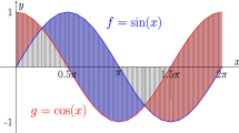
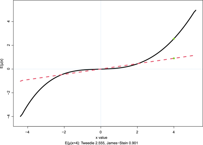
Fig. 2
Prostate data: Tweedie’s estimate of
E
{
μ
∣
x
}
, 5 degrees of freedom; dashed curve is James–Stein estimate
Full size image
The choice
J
=
5
was applied to the prostate cancer data of Fig.
1
: Tweedie’s formula (
14
) gave
μ
^
(
x
)
=
E
{
μ
∣
x
}
, graphed as the solid curve in Fig.
2
. It differs markedly from the James–Stein estimate
J
=
2
, the dashed line. At
x
=
4
for example, the
J
=
5
estimate is
Footnote
3
E
{
μ
∣
x
=
4
}
=
2.555
(18)
compared to 0.901 for the James–Stein estimate.
The estimated curve
E
{
μ
∣
x
}
is
empirical Bayes
in the same sense as (
8
): the parameter vector
β
was selected by maximum likelihood, as discussed next. With
J
=
5
, the prior was able to adapt to the “fishing expedition” nature of such microarray studies, where we expect most of the genes to be null or close to null, with
μ
i
nearly zero (corresponding here to the flat part of the curve for
x
between
−
2
and 2) and, hopefully, a small proportion of interestingly large
μ
i
s.
The sample size
n
=
6033
has much to do with Fig.
2
. James and Stein (
1961
) was usually considered in terms of small samples, perhaps
n
≤
20
, for which there would be little hope of seeing the detail in Fig.
2
. The term “machine learning era” seems less fanciful when considering the scale of problems statisticians are now asked to deal with, as well as the tools they use to solve them.
It looks like it might be hard work computing Fig.
2
but it’s not. The histogram in Fig.
1
has 97 bins, with centerpoints
v
v
=
(
−
4.4
,
−
4.3
,
…
,
5.1
,
5.2
)
.
(19)
Let
y
j
be the count in bin
j
, that is, the number of the 6033
x
i
values falling into it, with the vector of counts being
y
y
=
(
y
1
,
…
,
y
97
)
.
(20)
Then the single R command
l
l
^
=
log
(
glm
(
y
y
∼
poly
(
v
v
,
5
)
,
poisson
)
$
fit
)
(21)
provides a close approximation to the MLE of
log
f
(
x
)
in (
14
); numerical differentiation of
l
l
^
gives Tweedie’s estimate. Section 3.4 of Efron (
2023
) shows why Poisson regression (
21
) is appropriate here.
The James–Stein theorem depends on the independence assumption in (
1
), unlikely to be true in the microarray study, but the estimates (
2
) have a certain marginal validity even under dependence. This is clearer from the empirical Bayes point of view. The Tweedie estimate
x
i
+
l
^
′
(
x
i
)
requires only that
l
^
′
(
x
)
be close to
l
′
(
x
)
, not that it be estimated from independent
x
i
s.
Footnote
4
3
Shrinkage estimators
James and Stein’s paper aroused excited interest in the statistics community when it arrived in 1961. Most of the excitement focused on the strict inadmissibility of the traditional maximum likelihood estimate demonstrated by the James–Stein rule. Other rules dominating the MLE were discovered, for instance the Bayes estimator of Strawderman (
1971
), that was itself admissible while rendering the MLE inadmissible.
Big new ideas can take a while to make their true impact felt. The James–Stein rule had an influential side effect on subsequent theory and practice in that it demonstrated, in an inarguable way, the virtues of
shrinkage estimation
: given an ensemble of problems, individual estimates are shrunk toward a central point; that is, a deliberate bias is introduced, pulling estimates away from their MLEs for the sake of better group performances.
Admissibility and inadmissibility aren’t much in the air these days, while shrinkage estimation has gone on to play a major role in modern practice. A spectacular success story is the lasso (Tibshirani,
1996
). Lasso shrinkage is extreme, pulling some (often most) of the coefficient estimates all the way back to zero.
Bayes and empirical Bayes rules tend to be strong shrinkers. Tweedie’s estimate in Fig.
2
(
J
=
5
) shrinks the estimate of
E
{
μ
∣
x
=
4
}
from its MLE value 4 down to 2.555. For
μ
between
−
1
and 1, the shrinkage is almost all the way to zero.
The reader may have been surprised to see that neither Tweedie’s formula (
14
) for
E
{
μ
i
∣
x
i
}
nor its empirical version (
15
) require estimation of the prior
π
(
μ
)
. This is a special property of the posterior expectation
E
{
μ
i
∣
x
i
}
and isn’t available for say
Pr
{
μ
i
≥
2
∣
x
i
}
, or most other Bayesian targets.
“Bayesian deconvolution” (Efron,
2016
) uses low-dimensional parametric modeling of
π
(
μ
)
for general empirical Bayes computations. It was applied to finding a prior density
π
(
μ
)
that would give the distribution of
x
seen in Fig.
1
, assuming the normal sampling model (
1
). The deconvolution model for
π
(
μ
)
used a delta function at
μ
=
0
(for the “null” genes) and a natural spline function with four degrees of freedom for the non-null cases.
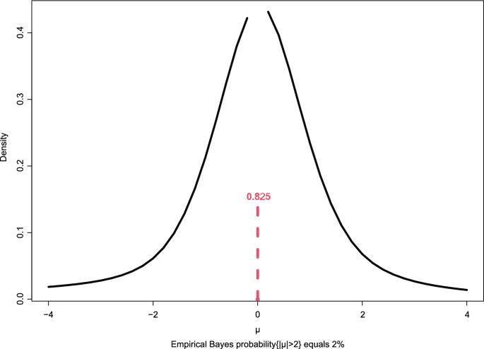
Fig. 3
Empirical Bayes conditional density of
μ
given
μ
not zero;
Pr
{
μ
=
0
}
equals 0.825
Full size image
The estimated prior
Footnote
5
π
^
(
μ
)
is shown in Fig.
3
; it put probability 0.825 on
μ
=
0
, while the conditional distribution given
μ
≠
0
was a moderately heavy-tailed version of
N
(
0
,
1.33
2
)
. Based on
π
^
(
μ
)
we can form estimates of
any
Bayesian target, for instance
Pr
^
{
μ
i
≥
2
∣
x
i
=
4
}
=
0.80
. Figure
3
is a direct descendent of the James–Stein rule, now 60-plus years on.
A less-direct descendent, but still on the family tree, arrived in 1995. The
false discovery rate
paper by Benjamini and Hochberg concerned simultaneous hypothesis testing. Looking at Fig.
1
, which of the
n
=
6033
genes can confidently be labeled as non-null, that is as having
μ
i
≠
0
?
Suppose for convenience that the
x
i
s are ordered from smallest to largest. The right-sided significance level for testing
μ
i
=
0
is
S
0
(
x
i
)
=
1
−
Φ
(
x
i
)
,
(22)
where
Φ
is the standard normal cumulative distribution function. Of the 6033 genes, 401 had
S
i
≤
0.05
, the usual rejection level for individual testing, but even if actually
all
of the genes were null we would expect 302 such rejections, so individual testing can’t be right. Benjamini and Hochberg proposed a novel simultaneous testing rule that safely controls the number of “false discoveries” — genes falsely labeled ”non-null” — while not being discouragingly strict. (My summary here won’t give the BH rule its full due; see Chapter 4 of Efron (
2010
) for a more complete description.)
Let
S
^
(
x
)
be the observed proportion of
x
i
s exceeding value
x
, and define
F
d
r
^
(
x
)
=
π
0
S
0
(
x
)
/
S
^
(
x
)
,
(23)
where
π
0
is the proportion of null genes among all
n
.
Footnote
6
For a fixed control level
α
, such as
α
=
0.1
, the BH rule says to reject the null hypothesis
μ
i
=
0
for those genes having
F
d
r
^
(
x
i
)
≤
α
.
(24)
The Benjamini–Hochberg theorem states that under independence assumptions like (
1
), the expected proportion of false discoveries by rule (
24
) is
α
.
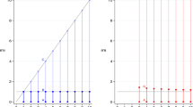
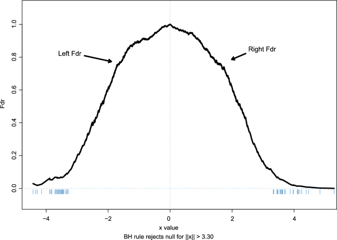
Fig. 4
Prostate data: left Fdr and right Fdr; dashes show 60 genes with
F
d
r
<
0.1
Full size image
Figure
4
shows
F
d
r
^
for the prostate cancer data and also for the left-sided Fdr estimate, where significance is defined by
S
0
(
x
i
)
=
Φ
(
x
i
)
rather than (
22
). I applied the BH rule with
α
=
0.1
which labeled 60 genes as non-null, 32 on the left and 28 on the right. The BH theorem says that we can expect 6 of the 60 to actually be null.
The fdr story has evolved very much along the lines of its James–Stein predecessor. Intense initial interest focused on the exact frequentist control of false discovery rates. The Bayes and empirical Bayes implications came later: as at (
5
), we assume that each
x
i
is a realization of a random variable
x
given by
μ
∼
π
(
μ
)
and
x
∣
μ
∼
p
(
x
∣
μ
)
,
(25)
where
p
(
x
∣
μ
)
is a known probability kernel which I’ll take here to be the normal sampling model (
1
). Then if
S
(
x
) is 1 minus the cdf of the marginal density (
13
), Bayes rule gives
Pr
{
μ
=
0
∣
x
}
=
π
0
S
0
(
x
)
/
S
(
x
)
.
(26)
Comparing (
26
) with (
23
) says that the BH rule amounts to labeling case
i
as non-null if its obvious empirical Bayes estimate of nullness is less than
α
. This is less precise than the frequentist control theorem but, as with the James–Stein estimator, is more robust in not demanding independence among the
x
i
s. The family resemblance between JS and BH is through shrinkage: in the BH case the shrinkage of significance levels. For instance,
x
i
=
3
has individual significance level 0.001 against nullness, whereas
F
d
r
^
=
0.164
for the prostate data, i.e, still with about a 1/6 chance of gene
i
being null.
So what does machine learning have to do with the James–Stein estimator? Nothing to its birth but, as the articles in this volume show, a great deal to its downstream effects on statistical theory and practice. Charles Stein, who was a good applied statistician when he put his mind to it, might have enjoyed these developments, but maybe not; his heart was always with the mathematics.
References
Benjamini, Y., & Hochberg, Y. (1995). Controlling the false discovery rate: A practical and powerful approach to multiple testing.
Journal of the Royal Statistical Society Series B,
57
(1), 289–300.
Article
MathSciNet
Google Scholar
Efron, B. (2010).
Large-scale inference: Empirical Bayes methods for estimation, testing, and prediction
(Vol. 1). Cambridge: Cambridge University Press.
Book
Google Scholar
Efron, B. (2011). Tweedie’s formula and selection bias.
Journal of the American Statistical Association,
106
(496), 1602–1614.
https://doi.org/10.1198/jasa.2011.tm11181
Article
MathSciNet
Google Scholar
Efron, B. (2016). Empirical Bayes deconvolution estimates.
Biometrika,
103
(1), 1–20.
https://doi.org/10.1093/biomet/asv068
Article
MathSciNet
Google Scholar
Efron, B. (2023).
Exponential Families in Theory and Practice
. Cambridge: Cambridge University Press.
Google Scholar
Efron, B., & Morris, C. (1973). Stein’s estimation rule and its competitors—An empirical Bayes approach.
Journal of the American Statistical Association,
68
, 117–130.
MathSciNet
Google Scholar
James, W., & Stein, C. (1961). Estimation with quadratic loss. In
Proc. 4th Berkeley Sympos. Math. Statist. and Prob.
(Vol. I, pp. 361–379). Berkeley: University of California Press.
Narasimhan, B., & Efron, B. (2020). deconvolveR: A G-Modeling Program for Deconvolution and Empirical Bayes Estimation.
Journal of Statistical Software,
94
(11), 1–20.
https://doi.org/10.18637/jss.v094.i11
Article
Google Scholar
Robbins, H. (1956). An empirical Bayes approach to statistics. In
Proc. 3rd Berkeley Sympos. Math. Statist. and Prob.
(Vol. I, pp. 157–163). Berkeley: University of California Press.
Strawderman, W. E. (1971). Proper Bayes minimax estimators of the multivariate normal mean.
Annals of Mathematical Statistics,
42
(1), 385–388.
https://doi.org/10.1214/aoms/1177693528
Article
MathSciNet
Google Scholar
Tibshirani, R. (1996). Regression shrinkage and selection via the lasso.
Journal of the Royal Statistical Society Series B,
58
(1), 267–288.
Article
MathSciNet
Google Scholar
Download references |
| Markdown | [Skip to main content](https://link.springer.com/article/10.1007/s42081-023-00209-y#main)
Advertisement
[](https://pubads.g.doubleclick.net/gampad/jump?iu=/270604982/springerlink/42081/article&sz=728x90&pos=top&articleid=s42081-023-00209-y)
[](https://link.springer.com/)
[Account](https://link.springer.com/article/10.1007/s42081-023-00209-y)
[Menu]()
[Find a journal](https://link.springer.com/journals/) [Publish with us](https://www.springernature.com/gp/authors) [Track your research](https://link.springernature.com/home/)
[Search]()
[Saved research](https://link.springer.com/saved-research)
[Cart](https://order.springer.com/public/cart)
## Search
## Navigation
- [Find a journal](https://link.springer.com/journals/)
- [Publish with us](https://www.springernature.com/gp/authors)
- [Track your research](https://link.springernature.com/home/)
1. [Home](https://link.springer.com/)
2. [Japanese Journal of Statistics and Data Science](https://link.springer.com/journal/42081)
3. Article
# Machine learning and the James–Stein estimator
- Original Paper
- Stein Estimation and Statistical Shrinkage Methods
- [Open access](https://www.springernature.com/gp/open-science/about/the-fundamentals-of-open-access-and-open-research)
- Published:
30 June 2023
- Volume 7, pages 257–266, (2024)
- [Cite this article](https://link.springer.com/article/10.1007/s42081-023-00209-y#citeas)
You have full access to this [open access](https://www.springernature.com/gp/open-science/about/the-fundamentals-of-open-access-and-open-research) article
[Download PDF](https://link.springer.com/content/pdf/10.1007/s42081-023-00209-y.pdf)
[Save article](https://link.springer.com/article/10.1007/s42081-023-00209-y/save-research?_csrf=MqX1VwflVBF2wGV6B4ITqKc5OgaOhi_J)
[View saved research](https://link.springer.com/saved-research)
[ Japanese Journal of Statistics and Data Science](https://link.springer.com/journal/42081)
[Aims and scope](https://link.springer.com/journal/42081/aims-and-scope)
[Submit manuscript](https://www.editorialmanager.com/jjsd)
Machine learning and the James–Stein estimator
[Download PDF](https://link.springer.com/content/pdf/10.1007/s42081-023-00209-y.pdf)
- [Bradley Efron](https://link.springer.com/article/10.1007/s42081-023-00209-y#auth-Bradley-Efron-Aff1-Aff2)
[1](https://link.springer.com/article/10.1007/s42081-023-00209-y#Aff1),[2](https://link.springer.com/article/10.1007/s42081-023-00209-y#Aff2)
- 9362 Accesses
- 7 Citations
- 24 Altmetric
- 1 Mention
- [Explore all metrics](https://link.springer.com/article/10.1007/s42081-023-00209-y/metrics)
## Abstract
It is now 62 years since the publication of James and Stein’s seminal article on the estimation of a multivariate normal mean vector. The paper made a spectacular first impression on the statistical community through its demonstration of inadmissability of the maximum likelihood estimator. It continues to be influential, but not for the initial reasons. Empirical Bayes shrinkage estimation, now a major topic, found its early justification in the James–Stein formula. Less obvious downstream topics include Tweedie’s formula and Benjamini and Hochberg’s false discovery rate algorithm. This is a short and mainly non-technical review of the James–Stein rule and its effects on the machine learning era of statistical innovation.
### Similar content being viewed by others
### [Expansion estimators improving the bias and risk of James–Stein’s shrinkage estimator](https://link.springer.com/10.1007/s42081-023-00227-w)
Article 16 December 2023
### [A new class of metrics for learning on real-valued and structured data](https://link.springer.com/10.1007/s10618-019-00622-6)
Article 27 March 2019
### [Weak Versus Strong Dominance of Shrinkage Estimators](https://link.springer.com/10.1007/s40953-021-00270-y)
Article 18 November 2021
### Explore related subjects
Discover the latest articles, books and news in related subjects, suggested using machine learning.
- [Bayesian Inference](https://link.springer.com/subjects/bayesian-inference)
- [Empiricism](https://link.springer.com/subjects/empiricism)
- [Machine Learning](https://link.springer.com/subjects/machine-learning)
- [Non-parametric Inference](https://link.springer.com/subjects/non-parametric-inference)
- [Statistical Learning](https://link.springer.com/subjects/statistical-learning)
- [Statistical Theory and Methods](https://link.springer.com/subjects/statistical-theory-and-methods)
- [Empirical Bayesian Methods in Statistical Inference](https://link.springer.com/subjects/empirical-bayesian-methods-in-statistical-inference)
## 1 Introduction
By and large, the statistics world is one of heuristics, approximations, and asymptotics. The James–Stein estimator arrived in that world in 1961 on a note of startling specificity: unseen parameters μ 1 , μ 2 , … , μ n produce independent observations
x
i
∼
ind
N
(
μ
i
,
1
)
,
i
\=
1
,
…
,
n
,
(1)
n ≥ 3. The James–Stein rule in its simplest form proposed estimating the μ i by
μ
^
i
J
S
\=
(
1
−
n
−
2
S
)
x
i
(
S
\=
∑
i
\=
1
n
x
i
2
)
.
(2)
Formula ([2](https://link.springer.com/article/10.1007/s42081-023-00209-y#Equ2)) looked implausible: the estimate of μ i depended on the *other* observations x j, j ≠ i (through *S*), as well as x i, despite the independence assumption. Nevertheless, James and Stein showed that Rule ([2](https://link.springer.com/article/10.1007/s42081-023-00209-y#Equ2)) *always* beat the obvious maximum likelihood estimates
μ
^
i
M
L
\=
x
¯
i
(
i
\=
1
,
…
,
n
)
(3)
in terms of total expected squared error
E
{
∑
i
\=
1
n
(
μ
^
i
−
μ
i
)
2
}
.
(4)
That “always” was the shocking part: two centuries of statistical theory, ANOVA, regression, multivariate analysis, etc., depended on maximum likelihood estimation. Did everything have to be rethought?
One path forward involved Bayesian thinking. If we assumed that the μ i themselves came from a normal distribution,
μ
i
∼
ind
N
(
0
,
A
)
for
i
\=
1
,
…
,
n
,
(5)
with variance A ≥ 0, the Bayes estimates would be
μ
^
i
B
a
y
e
s
\=
B
x
i
(
B
\=
A
/
(
A
\+
1
)
)
.
(6)
We don’t know *A* or *B* but
B
^
\=
1
−
(
n
−
2
)
/
S
(7)
is *B*’s unbiased estimate: we can rewrite ([2](https://link.springer.com/article/10.1007/s42081-023-00209-y#Equ2)) as
μ
^
i
J
S
\=
B
^
x
i
,
(8)
which at least looks more plausible.
In the language introduced by Robbins ([1956](https://link.springer.com/article/10.1007/s42081-023-00209-y#ref-CR9 "Robbins, H. (1956). An empirical Bayes approach to statistics. In Proc. 3rd Berkeley Sympos. Math. Statist. and Prob. (Vol. I, pp. 157–163). Berkeley: University of California Press.")), formula ([8](https://link.springer.com/article/10.1007/s42081-023-00209-y#Equ8)) is an *empirical Bayes* estimator, another shocking post-war statistical innovation. Carl Morris and I wrote a series of papers in the 1970 s exploring Bayesian roots of the James–Stein estimator (Efron and Morris, [1973](https://link.springer.com/article/10.1007/s42081-023-00209-y#ref-CR6 "Efron, B., & Morris, C. (1973). Stein’s estimation rule and its competitors—An empirical Bayes approach. Journal of the American Statistical Association, 68, 117–130.")). Something is lost in the empirical Bayes formulation, namely the frequentist “always” of expected square error minimization, but a lot is gained in flexibility and scope, as discussed in Sect. [2](https://link.springer.com/article/10.1007/s42081-023-00209-y#Sec2).
**Fig. 1**
[](https://link.springer.com/article/10.1007/s42081-023-00209-y/figures/1)
Prostate data: 6033 *x* values; mean 0.003, sd \= 1\.135; curve is proportional to a N ( 0 , 1 ) density
[Full size image](https://link.springer.com/article/10.1007/s42081-023-00209-y/figures/1)
Figure [1](https://link.springer.com/article/10.1007/s42081-023-00209-y#Fig1) illustrates an example of simultaneous estimation pursued in Sect. 2.1 of Efron ([2010](https://link.springer.com/article/10.1007/s42081-023-00209-y#ref-CR2 "Efron, B. (2010). Large-scale inference: Empirical Bayes methods for estimation, testing, and prediction (Vol. 1). Cambridge: Cambridge University Press.")). A microarray study has compared expression levels between prostate cancer patients and control subjects for n \= 6033 genes. For each gene, a statistic x i has been calculated (essentially a “*z*\-value”),
x
i
∼
N
(
μ
i
,
1
)
,
i
\=
1
,
…
,
n
,
(9)
where μ i measures the difference between cancer and control group levels.
The solid curve in Fig. [1](https://link.springer.com/article/10.1007/s42081-023-00209-y#Fig1) is a N ( 0 , 1 ) density scaled to have the same area as the histogram of the 6033 *x* values. A bad result from the researchers’ point of view would be a perfect fit of curve to histogram, which would imply all the genes have μ i \= 0, the “null” value of no difference between cancer patients and controls.
That’s not what happened: the histogram has mildly heavy tails in both directions. The researchers were hoping to find genes with large values of ‖ μ i ‖—ones that might be a clue to prostate cancer etiology—as suggested by the heavy tails. How encouraged should they be?
Not very, according to the James–Stein rule. The 6033 x i values have mean 0.003, which I’ll take to be zero, and empirical variance
σ
^
2
\=
1\.289.
(10)
The James–Stein estimate ([2](https://link.springer.com/article/10.1007/s42081-023-00209-y#Equ2)) is
μ
^
i
J
S
\=
(
1
−
n
−
2
n
−
1
1
σ
^
2
)
x
i
\=
0\.224
⋅
x
i
,
(11)
so even x i \= 5 yields an estimate barely exceeding 1. Section [2](https://link.springer.com/article/10.1007/s42081-023-00209-y#Sec2) suggests a more optimistic analysis.
## 2 Tweedie’s formula
The impressive precision of the James–Stein theorem came at a cost in generality. Efforts to extend the theorem, say to Poisson rather than normal observations, or to measures of loss other than total squared error, gave encouraging asymptotic results but not the James–Stein kind of finite sample frequentist dominance.
Better progress was possible on the empirical Bayes side of the street. *Tweedie’s formula* (Efron, [2011](https://link.springer.com/article/10.1007/s42081-023-00209-y#ref-CR3 "Efron, B. (2011). Tweedie’s formula and selection bias. Journal of the American Statistical Association, 106(496), 1602–1614.
https://doi.org/10.1198/jasa.2011.tm11181
")) has been particularly useful. We wish to calculate Bayesian estimates
μ
i
B
a
y
e
s
\=
E
{
μ
i
∣
x
i
}
,
i
\=
1
,
…
,
n
,
(12)
in the normal sampling model ([1](https://link.springer.com/article/10.1007/s42081-023-00209-y#Equ1)), starting from a given (possibly non-normal) prior π ( μ ), applying to all *n* cases. Let *f*(*x*) be the marginal density
f
(
x
)
\=
∫
R
π
(
μ
)
ϕ
(
x
−
μ
)
d
μ
,
(13)
with ϕ the standard N ( 0 , 1 ) density and R the range of μ. (It isn’t necessary for π ( ⋅ ) to be a continuous distribution but it simplifies notation.)
Tweedie’s formula provides an elegant statement for μ i B a y e s, the posterior expectation of μ i given x i,
μ
i
B
a
y
e
s
\=
E
{
μ
i
∣
x
i
}
\=
x
i
\+
l
′
(
x
i
)
with
l
′
(
x
i
)
\=
d
d
x
log
(
f
(
x
i
)
)
.
(14)
In the empirical Bayes situation ([1](https://link.springer.com/article/10.1007/s42081-023-00209-y#Equ1)), where the prior π ( ⋅ ) is unknown, we can use the observed data x 1 , … , x n to estimate the marginal density *f*(*x*), say by f ^ ( x ), giving empirical Bayes estimates
μ
^
i
\=
x
i
\+
l
^
′
(
x
i
)
.
(15)
The Bayes estimate ([14](https://link.springer.com/article/10.1007/s42081-023-00209-y#Equ14)) can be thought of as the MLE x i plus a Bayesian correction term l ′ ( x i ). When the prior π ( μ ) is the N ( 0 , A ) distribution ([5](https://link.springer.com/article/10.1007/s42081-023-00209-y#Equ5)), μ i B a y e s equals B x i ([6](https://link.springer.com/article/10.1007/s42081-023-00209-y#Equ6)). Simple formulas for μ i B a y e s give out for most other choices of π ( μ ) but now, in the machine learning era[Footnote 1](https://link.springer.com/article/10.1007/s42081-023-00209-y#Fn1) of statistical research, numerical methods provide useful ways forward, as discussed next.
The *log polynomial class*[Footnote 2](https://link.springer.com/article/10.1007/s42081-023-00209-y#Fn2) of marginal densities defines *f*(*x*) by
log
(
f
β
(
x
)
)
\=
β
0
\+
β
⊤
c
(
x
)
.
(16)
Here
c
(
x
)
\=
(
x
,
x
2
,
…
,
x
J
)
⊤
and
β
\=
(
β
1
,
…
,
β
J
)
⊤
,
(17)
with β 0 chosen to make f β ( x ) integrate to 1. The choice J \= 2 gives normal marginals; larger values of *J* allow for marginal non-normality.
**Fig. 2**
[](https://link.springer.com/article/10.1007/s42081-023-00209-y/figures/2)
Prostate data: Tweedie’s estimate of E { μ ∣ x }, 5 degrees of freedom; dashed curve is James–Stein estimate
[Full size image](https://link.springer.com/article/10.1007/s42081-023-00209-y/figures/2)
The choice J \= 5 was applied to the prostate cancer data of Fig. [1](https://link.springer.com/article/10.1007/s42081-023-00209-y#Fig1): Tweedie’s formula ([14](https://link.springer.com/article/10.1007/s42081-023-00209-y#Equ14)) gave μ ^ ( x ) \= E { μ ∣ x }, graphed as the solid curve in Fig. [2](https://link.springer.com/article/10.1007/s42081-023-00209-y#Fig2). It differs markedly from the James–Stein estimate J \= 2, the dashed line. At x \= 4 for example, the J \= 5 estimate is[Footnote 3](https://link.springer.com/article/10.1007/s42081-023-00209-y#Fn3)
E
{
μ
∣
x
\=
4
}
\=
2\.555
(18)
compared to 0.901 for the James–Stein estimate.
The estimated curve E { μ ∣ x } is *empirical Bayes* in the same sense as ([8](https://link.springer.com/article/10.1007/s42081-023-00209-y#Equ8)): the parameter vector β was selected by maximum likelihood, as discussed next. With J \= 5, the prior was able to adapt to the “fishing expedition” nature of such microarray studies, where we expect most of the genes to be null or close to null, with μ i nearly zero (corresponding here to the flat part of the curve for *x* between − 2 and 2) and, hopefully, a small proportion of interestingly large μ is.
The sample size n \= 6033 has much to do with Fig. [2](https://link.springer.com/article/10.1007/s42081-023-00209-y#Fig2). James and Stein ([1961](https://link.springer.com/article/10.1007/s42081-023-00209-y#ref-CR7 "James, W., & Stein, C. (1961). Estimation with quadratic loss. In Proc. 4th Berkeley Sympos. Math. Statist. and Prob. (Vol. I, pp. 361–379). Berkeley: University of California Press.")) was usually considered in terms of small samples, perhaps n ≤ 20, for which there would be little hope of seeing the detail in Fig. [2](https://link.springer.com/article/10.1007/s42081-023-00209-y#Fig2). The term “machine learning era” seems less fanciful when considering the scale of problems statisticians are now asked to deal with, as well as the tools they use to solve them.
It looks like it might be hard work computing Fig. [2](https://link.springer.com/article/10.1007/s42081-023-00209-y#Fig2) but it’s not. The histogram in Fig. [1](https://link.springer.com/article/10.1007/s42081-023-00209-y#Fig1) has 97 bins, with centerpoints
v
v
\=
(
−
4\.4
,
−
4\.3
,
…
,
5\.1
,
5\.2
)
.
(19)
Let y j be the count in bin *j*, that is, the number of the 6033 x i values falling into it, with the vector of counts being
y
y
\=
(
y
1
,
…
,
y
97
)
.
(20)
Then the single R command
l
l
^
\=
log
(
glm
(
y
y
∼
poly
(
v
v
,
5
)
,
poisson
)
\$
fit
)
(21)
provides a close approximation to the MLE of log f ( x ) in ([14](https://link.springer.com/article/10.1007/s42081-023-00209-y#Equ14)); numerical differentiation of l l ^ gives Tweedie’s estimate. Section 3.4 of Efron ([2023](https://link.springer.com/article/10.1007/s42081-023-00209-y#ref-CR5 "Efron, B. (2023). Exponential Families in Theory and Practice. Cambridge: Cambridge University Press.")) shows why Poisson regression ([21](https://link.springer.com/article/10.1007/s42081-023-00209-y#Equ21)) is appropriate here.
The James–Stein theorem depends on the independence assumption in ([1](https://link.springer.com/article/10.1007/s42081-023-00209-y#Equ1)), unlikely to be true in the microarray study, but the estimates ([2](https://link.springer.com/article/10.1007/s42081-023-00209-y#Equ2)) have a certain marginal validity even under dependence. This is clearer from the empirical Bayes point of view. The Tweedie estimate x i \+ l ^ ′ ( x i ) requires only that l ^ ′ ( x ) be close to l ′ ( x ), not that it be estimated from independent x is.[Footnote 4](https://link.springer.com/article/10.1007/s42081-023-00209-y#Fn4)
## 3 Shrinkage estimators
James and Stein’s paper aroused excited interest in the statistics community when it arrived in 1961. Most of the excitement focused on the strict inadmissibility of the traditional maximum likelihood estimate demonstrated by the James–Stein rule. Other rules dominating the MLE were discovered, for instance the Bayes estimator of Strawderman ([1971](https://link.springer.com/article/10.1007/s42081-023-00209-y#ref-CR10 "Strawderman, W. E. (1971). Proper Bayes minimax estimators of the multivariate normal mean. Annals of Mathematical Statistics, 42(1), 385–388.
https://doi.org/10.1214/aoms/1177693528
")), that was itself admissible while rendering the MLE inadmissible.
Big new ideas can take a while to make their true impact felt. The James–Stein rule had an influential side effect on subsequent theory and practice in that it demonstrated, in an inarguable way, the virtues of *shrinkage estimation*: given an ensemble of problems, individual estimates are shrunk toward a central point; that is, a deliberate bias is introduced, pulling estimates away from their MLEs for the sake of better group performances.
Admissibility and inadmissibility aren’t much in the air these days, while shrinkage estimation has gone on to play a major role in modern practice. A spectacular success story is the lasso (Tibshirani, [1996](https://link.springer.com/article/10.1007/s42081-023-00209-y#ref-CR11 "Tibshirani, R. (1996). Regression shrinkage and selection via the lasso. Journal of the Royal Statistical Society Series B, 58(1), 267–288.")). Lasso shrinkage is extreme, pulling some (often most) of the coefficient estimates all the way back to zero.
Bayes and empirical Bayes rules tend to be strong shrinkers. Tweedie’s estimate in Fig. [2](https://link.springer.com/article/10.1007/s42081-023-00209-y#Fig2) (J \= 5) shrinks the estimate of E { μ ∣ x \= 4 } from its MLE value 4 down to 2.555. For μ between − 1 and 1, the shrinkage is almost all the way to zero.
The reader may have been surprised to see that neither Tweedie’s formula ([14](https://link.springer.com/article/10.1007/s42081-023-00209-y#Equ14)) for E { μ i ∣ x i } nor its empirical version ([15](https://link.springer.com/article/10.1007/s42081-023-00209-y#Equ15)) require estimation of the prior π ( μ ). This is a special property of the posterior expectation E { μ i ∣ x i } and isn’t available for say Pr { μ i ≥ 2 ∣ x i }, or most other Bayesian targets.
“Bayesian deconvolution” (Efron, [2016](https://link.springer.com/article/10.1007/s42081-023-00209-y#ref-CR4 "Efron, B. (2016). Empirical Bayes deconvolution estimates. Biometrika, 103(1), 1–20.
https://doi.org/10.1093/biomet/asv068
")) uses low-dimensional parametric modeling of π ( μ ) for general empirical Bayes computations. It was applied to finding a prior density π ( μ ) that would give the distribution of *x* seen in Fig. [1](https://link.springer.com/article/10.1007/s42081-023-00209-y#Fig1), assuming the normal sampling model ([1](https://link.springer.com/article/10.1007/s42081-023-00209-y#Equ1)). The deconvolution model for π ( μ ) used a delta function at μ \= 0 (for the “null” genes) and a natural spline function with four degrees of freedom for the non-null cases.
**Fig. 3**
[](https://link.springer.com/article/10.1007/s42081-023-00209-y/figures/3)
Empirical Bayes conditional density of μ given μ not zero; Pr { μ \= 0 } equals 0.825
[Full size image](https://link.springer.com/article/10.1007/s42081-023-00209-y/figures/3)
The estimated prior[Footnote 5](https://link.springer.com/article/10.1007/s42081-023-00209-y#Fn5)π ^ ( μ ) is shown in Fig. [3](https://link.springer.com/article/10.1007/s42081-023-00209-y#Fig3); it put probability 0.825 on μ \= 0, while the conditional distribution given μ ≠ 0 was a moderately heavy-tailed version of N ( 0 , 1\.33 2 ). Based on π ^ ( μ ) we can form estimates of *any* Bayesian target, for instance Pr ^ { μ i ≥ 2 ∣ x i \= 4 } \= 0\.80. Figure [3](https://link.springer.com/article/10.1007/s42081-023-00209-y#Fig3) is a direct descendent of the James–Stein rule, now 60-plus years on.
A less-direct descendent, but still on the family tree, arrived in 1995. The *false discovery rate* paper by Benjamini and Hochberg concerned simultaneous hypothesis testing. Looking at Fig. [1](https://link.springer.com/article/10.1007/s42081-023-00209-y#Fig1), which of the n \= 6033 genes can confidently be labeled as non-null, that is as having μ i ≠ 0?
Suppose for convenience that the x is are ordered from smallest to largest. The right-sided significance level for testing μ i \= 0 is
S
0
(
x
i
)
\=
1
−
Φ
(
x
i
)
,
(22)
where Φ is the standard normal cumulative distribution function. Of the 6033 genes, 401 had S i ≤ 0\.05, the usual rejection level for individual testing, but even if actually *all* of the genes were null we would expect 302 such rejections, so individual testing can’t be right. Benjamini and Hochberg proposed a novel simultaneous testing rule that safely controls the number of “false discoveries” — genes falsely labeled ”non-null” — while not being discouragingly strict. (My summary here won’t give the BH rule its full due; see Chapter 4 of Efron ([2010](https://link.springer.com/article/10.1007/s42081-023-00209-y#ref-CR2 "Efron, B. (2010). Large-scale inference: Empirical Bayes methods for estimation, testing, and prediction (Vol. 1). Cambridge: Cambridge University Press.")) for a more complete description.)
Let S ^ ( x ) be the observed proportion of x is exceeding value *x*, and define
F
d
r
^
(
x
)
\=
π
0
S
0
(
x
)
/
S
^
(
x
)
,
(23)
where π 0 is the proportion of null genes among all *n*.[Footnote 6](https://link.springer.com/article/10.1007/s42081-023-00209-y#Fn6) For a fixed control level α, such as α \= 0\.1, the BH rule says to reject the null hypothesis μ i \= 0 for those genes having
F
d
r
^
(
x
i
)
≤
α
.
(24)
The Benjamini–Hochberg theorem states that under independence assumptions like ([1](https://link.springer.com/article/10.1007/s42081-023-00209-y#Equ1)), the expected proportion of false discoveries by rule ([24](https://link.springer.com/article/10.1007/s42081-023-00209-y#Equ24)) is α.
**Fig. 4**
[](https://link.springer.com/article/10.1007/s42081-023-00209-y/figures/4)
Prostate data: left Fdr and right Fdr; dashes show 60 genes with F d r \< 0\.1
[Full size image](https://link.springer.com/article/10.1007/s42081-023-00209-y/figures/4)
Figure [4](https://link.springer.com/article/10.1007/s42081-023-00209-y#Fig4) shows F d r ^ for the prostate cancer data and also for the left-sided Fdr estimate, where significance is defined by S 0 ( x i ) \= Φ ( x i ) rather than ([22](https://link.springer.com/article/10.1007/s42081-023-00209-y#Equ22)). I applied the BH rule with α \= 0\.1 which labeled 60 genes as non-null, 32 on the left and 28 on the right. The BH theorem says that we can expect 6 of the 60 to actually be null.
The fdr story has evolved very much along the lines of its James–Stein predecessor. Intense initial interest focused on the exact frequentist control of false discovery rates. The Bayes and empirical Bayes implications came later: as at ([5](https://link.springer.com/article/10.1007/s42081-023-00209-y#Equ5)), we assume that each x i is a realization of a random variable *x* given by
μ
∼
π
(
μ
)
and
x
∣
μ
∼
p
(
x
∣
μ
)
,
(25)
where p ( x ∣ μ ) is a known probability kernel which I’ll take here to be the normal sampling model ([1](https://link.springer.com/article/10.1007/s42081-023-00209-y#Equ1)). Then if *S*(*x*) is 1 minus the cdf of the marginal density ([13](https://link.springer.com/article/10.1007/s42081-023-00209-y#Equ13)), Bayes rule gives
Pr
{
μ
\=
0
∣
x
}
\=
π
0
S
0
(
x
)
/
S
(
x
)
.
(26)
Comparing ([26](https://link.springer.com/article/10.1007/s42081-023-00209-y#Equ26)) with ([23](https://link.springer.com/article/10.1007/s42081-023-00209-y#Equ23)) says that the BH rule amounts to labeling case *i* as non-null if its obvious empirical Bayes estimate of nullness is less than α. This is less precise than the frequentist control theorem but, as with the James–Stein estimator, is more robust in not demanding independence among the x is. The family resemblance between JS and BH is through shrinkage: in the BH case the shrinkage of significance levels. For instance, x i \= 3 has individual significance level 0.001 against nullness, whereas F d r ^ \= 0\.164 for the prostate data, i.e, still with about a 1/6 chance of gene *i* being null.
So what does machine learning have to do with the James–Stein estimator? Nothing to its birth but, as the articles in this volume show, a great deal to its downstream effects on statistical theory and practice. Charles Stein, who was a good applied statistician when he put his mind to it, might have enjoyed these developments, but maybe not; his heart was always with the mathematics.
## Notes
1. Where algorithms can substitute for theorems.
2. For general use, a natural spline basis is preferable to polynomials, to control the behavior of log π ( μ ) at the extremes.
3. With an estimated bootstrap standard error of 0.192.
4. The accuracy of the Tweedie estimate *does* suffer under dependence, so the previously quoted bootstrap standard error is likely to be optimistic.
5. Estimated using the CRAN package deconvolveR (Narasimhan and Efron, [2020](https://link.springer.com/article/10.1007/s42081-023-00209-y#ref-CR8 "Narasimhan, B., & Efron, B. (2020). deconvolveR: A G-Modeling Program for Deconvolution and Empirical Bayes Estimation. Journal of Statistical Software, 94(11), 1–20.
https://doi.org/10.18637/jss.v094.i11
")).
6. π 0 can be estimated but in practice it is usually replaced by its upper bound 1 in applying rule ([24](https://link.springer.com/article/10.1007/s42081-023-00209-y#Equ24)). For cases like the prostate data where most of the genes are null, this doesn’t much affect the outcome.
## References
- Benjamini, Y., & Hochberg, Y. (1995). Controlling the false discovery rate: A practical and powerful approach to multiple testing. *Journal of the Royal Statistical Society Series B,* *57*(1), 289–300.
[Article](https://doi.org/10.1111%2Fj.2517-6161.1995.tb02031.x) [MathSciNet](http://www.ams.org/mathscinet-getitem?mr=1325392) [Google Scholar](http://scholar.google.com/scholar_lookup?&title=Controlling%20the%20false%20discovery%20rate%3A%20A%20practical%20and%20powerful%20approach%20to%20multiple%20testing&journal=Journal%20of%20the%20Royal%20Statistical%20Society%20Series%20B&doi=10.1111%2Fj.2517-6161.1995.tb02031.x&volume=57&issue=1&pages=289-300&publication_year=1995&author=Benjamini%2CY&author=Hochberg%2CY)
- Efron, B. (2010). *Large-scale inference: Empirical Bayes methods for estimation, testing, and prediction* (Vol. 1). Cambridge: Cambridge University Press.
[Book](https://doi.org/10.1017%2FCBO9780511761362) [Google Scholar](http://scholar.google.com/scholar_lookup?&title=Large-scale%20inference%3A%20Empirical%20Bayes%20methods%20for%20estimation%2C%20testing%2C%20and%20prediction&doi=10.1017%2FCBO9780511761362&publication_year=2010&author=Efron%2CB)
- Efron, B. (2011). Tweedie’s formula and selection bias. *Journal of the American Statistical Association,* *106*(496), 1602–1614. <https://doi.org/10.1198/jasa.2011.tm11181>
[Article](https://doi.org/10.1198%2Fjasa.2011.tm11181) [MathSciNet](http://www.ams.org/mathscinet-getitem?mr=2896860) [Google Scholar](http://scholar.google.com/scholar_lookup?&title=Tweedie%E2%80%99s%20formula%20and%20selection%20bias&journal=Journal%20of%20the%20American%20Statistical%20Association&doi=10.1198%2Fjasa.2011.tm11181&volume=106&issue=496&pages=1602-1614&publication_year=2011&author=Efron%2CB)
- Efron, B. (2016). Empirical Bayes deconvolution estimates. *Biometrika,* *103*(1), 1–20. <https://doi.org/10.1093/biomet/asv068>
[Article](https://doi.org/10.1093%2Fbiomet%2Fasv068) [MathSciNet](http://www.ams.org/mathscinet-getitem?mr=3465818) [Google Scholar](http://scholar.google.com/scholar_lookup?&title=Empirical%20Bayes%20deconvolution%20estimates&journal=Biometrika&doi=10.1093%2Fbiomet%2Fasv068&volume=103&issue=1&pages=1-20&publication_year=2016&author=Efron%2CB)
- Efron, B. (2023). *Exponential Families in Theory and Practice*. Cambridge: Cambridge University Press.
[Google Scholar](http://scholar.google.com/scholar_lookup?&title=Exponential%20Families%20in%20Theory%20and%20Practice&publication_year=2023&author=Efron%2CB)
- Efron, B., & Morris, C. (1973). Stein’s estimation rule and its competitors—An empirical Bayes approach. *Journal of the American Statistical Association,* *68*, 117–130.
[MathSciNet](http://www.ams.org/mathscinet-getitem?mr=388597) [Google Scholar](http://scholar.google.com/scholar_lookup?&title=Stein%E2%80%99s%20estimation%20rule%20and%20its%20competitors%E2%80%94An%20empirical%20Bayes%20approach&journal=Journal%20of%20the%20American%20Statistical%20Association&volume=68&pages=117-130&publication_year=1973&author=Efron%2CB&author=Morris%2CC)
- James, W., & Stein, C. (1961). Estimation with quadratic loss. In *Proc. 4th Berkeley Sympos. Math. Statist. and Prob.* (Vol. I, pp. 361–379). Berkeley: University of California Press.
- Narasimhan, B., & Efron, B. (2020). deconvolveR: A G-Modeling Program for Deconvolution and Empirical Bayes Estimation. *Journal of Statistical Software,* *94*(11), 1–20. <https://doi.org/10.18637/jss.v094.i11>
[Article](https://doi.org/10.18637%2Fjss.v094.i11) [Google Scholar](http://scholar.google.com/scholar_lookup?&title=deconvolveR%3A%20A%20G-Modeling%20Program%20for%20Deconvolution%20and%20Empirical%20Bayes%20Estimation&journal=Journal%20of%20Statistical%20Software&doi=10.18637%2Fjss.v094.i11&volume=94&issue=11&pages=1-20&publication_year=2020&author=Narasimhan%2CB&author=Efron%2CB)
- Robbins, H. (1956). An empirical Bayes approach to statistics. In *Proc. 3rd Berkeley Sympos. Math. Statist. and Prob.* (Vol. I, pp. 157–163). Berkeley: University of California Press.
- Strawderman, W. E. (1971). Proper Bayes minimax estimators of the multivariate normal mean. *Annals of Mathematical Statistics,* *42*(1), 385–388. <https://doi.org/10.1214/aoms/1177693528>
[Article](https://doi.org/10.1214%2Faoms%2F1177693528) [MathSciNet](http://www.ams.org/mathscinet-getitem?mr=397939) [Google Scholar](http://scholar.google.com/scholar_lookup?&title=Proper%20Bayes%20minimax%20estimators%20of%20the%20multivariate%20normal%20mean&journal=Annals%20of%20Mathematical%20Statistics&doi=10.1214%2Faoms%2F1177693528&volume=42&issue=1&pages=385-388&publication_year=1971&author=Strawderman%2CWE)
- Tibshirani, R. (1996). Regression shrinkage and selection via the lasso. *Journal of the Royal Statistical Society Series B,* *58*(1), 267–288.
[Article](https://doi.org/10.1111%2Fj.2517-6161.1996.tb02080.x) [MathSciNet](http://www.ams.org/mathscinet-getitem?mr=1379242) [Google Scholar](http://scholar.google.com/scholar_lookup?&title=Regression%20shrinkage%20and%20selection%20via%20the%20lasso&journal=Journal%20of%20the%20Royal%20Statistical%20Society%20Series%20B&doi=10.1111%2Fj.2517-6161.1996.tb02080.x&volume=58&issue=1&pages=267-288&publication_year=1996&author=Tibshirani%2CR)
[Download references](https://citation-needed.springer.com/v2/references/10.1007/s42081-023-00209-y?format=refman&flavour=references)
## Funding
No funds, grants, or other support was received.
## Author information
### Authors and Affiliations
1. Department of Statistics, Stanford University, 390 Jane Stanford Way, Stanford, CA, 94305, USA
Bradley Efron
2. Department of Biomedical Data Science, Stanford School of Medicine, 1265 Welch Road, Stanford, CA, 94305, USA
Bradley Efron
Authors
1. Bradley Efron
[View author publications](https://link.springer.com/search?sortBy=newestFirst&contributor=Bradley%20Efron)
Search author on:[PubMed](https://www.ncbi.nlm.nih.gov/entrez/query.fcgi?cmd=search&term=Bradley%20Efron) [Google Scholar](https://scholar.google.co.uk/scholar?as_q=&num=10&btnG=Search+Scholar&as_epq=&as_oq=&as_eq=&as_occt=any&as_sauthors=%22Bradley%20Efron%22&as_publication=&as_ylo=&as_yhi=&as_allsubj=all&hl=en)
### Corresponding author
Correspondence to [Bradley Efron](mailto:efron@stanford.edu).
## Ethics declarations
### Conflict of interest
The author has no relevant financial or non-financial interests to disclose.
## Additional information
### Publisher's Note
Springer Nature remains neutral with regard to jurisdictional claims in published maps and institutional affiliations.
Dedicated to the memory of Carl Morris.
## Rights and permissions
**Open Access** This article is licensed under a Creative Commons Attribution 4.0 International License, which permits use, sharing, adaptation, distribution and reproduction in any medium or format, as long as you give appropriate credit to the original author(s) and the source, provide a link to the Creative Commons licence, and indicate if changes were made. The images or other third party material in this article are included in the article’s Creative Commons licence, unless indicated otherwise in a credit line to the material. If material is not included in the article’s Creative Commons licence and your intended use is not permitted by statutory regulation or exceeds the permitted use, you will need to obtain permission directly from the copyright holder. To view a copy of this licence, visit <http://creativecommons.org/licenses/by/4.0/>.
[Reprints and permissions](https://s100.copyright.com/AppDispatchServlet?title=Machine%20learning%20and%20the%20James%E2%80%93Stein%20estimator&author=Bradley%20Efron&contentID=10.1007%2Fs42081-023-00209-y©right=The%20Author%28s%29&publication=2520-8756&publicationDate=2023-06-30&publisherName=SpringerNature&orderBeanReset=true&oa=CC%20BY)
## About this article
[](https://crossmark.crossref.org/dialog/?doi=10.1007/s42081-023-00209-y)
### Cite this article
Efron, B. Machine learning and the James–Stein estimator. *Jpn J Stat Data Sci* **7**, 257–266 (2024). https://doi.org/10.1007/s42081-023-00209-y
[Download citation](https://citation-needed.springer.com/v2/references/10.1007/s42081-023-00209-y?format=refman&flavour=citation)
- Received: 24 March 2023
- Accepted: 13 May 2023
- Published: 30 June 2023
- Version of record: 30 June 2023
- Issue date: June 2024
- DOI: https://doi.org/10.1007/s42081-023-00209-y
### Share this article
Anyone you share the following link with will be able to read this content:
Get shareable link
Sorry, a shareable link is not currently available for this article.
Copy shareable link to clipboard
Provided by the Springer Nature SharedIt content-sharing initiative
### Keywords
- [Empirical bayes](https://link.springer.com/search?query=Empirical%20bayes&facet-discipline="Statistics")
- [Shrinkage](https://link.springer.com/search?query=Shrinkage&facet-discipline="Statistics")
- [Tweedie’s formula](https://link.springer.com/search?query=Tweedie%E2%80%99s%20formula&facet-discipline="Statistics")
- [Benjamini–Hochberg algorithm](https://link.springer.com/search?query=Benjamini%E2%80%93Hochberg%20algorithm&facet-discipline="Statistics")
- Sections
- Figures
- References
- [Abstract](https://link.springer.com/article/10.1007/s42081-023-00209-y#Abs1)
- [1 Introduction](https://link.springer.com/article/10.1007/s42081-023-00209-y#Sec1)
- [2 Tweedie’s formula](https://link.springer.com/article/10.1007/s42081-023-00209-y#Sec2)
- [3 Shrinkage estimators](https://link.springer.com/article/10.1007/s42081-023-00209-y#Sec3)
- [Notes](https://link.springer.com/article/10.1007/s42081-023-00209-y#notes)
- [References](https://link.springer.com/article/10.1007/s42081-023-00209-y#Bib1)
- [Funding](https://link.springer.com/article/10.1007/s42081-023-00209-y#Fun)
- [Author information](https://link.springer.com/article/10.1007/s42081-023-00209-y#author-information)
- [Ethics declarations](https://link.springer.com/article/10.1007/s42081-023-00209-y#ethics)
- [Additional information](https://link.springer.com/article/10.1007/s42081-023-00209-y#additional-information)
- [Rights and permissions](https://link.springer.com/article/10.1007/s42081-023-00209-y#rightslink)
- [About this article](https://link.springer.com/article/10.1007/s42081-023-00209-y#article-info)
Advertisement
- **Fig. 1**
![Fig. 1]()
[View in article](https://link.springer.com/article/10.1007/s42081-023-00209-y#Fig1)[Full size image](https://link.springer.com/article/10.1007/s42081-023-00209-y/figures/1)
- **Fig. 2**
![Fig. 2]()
[View in article](https://link.springer.com/article/10.1007/s42081-023-00209-y#Fig2)[Full size image](https://link.springer.com/article/10.1007/s42081-023-00209-y/figures/2)
- **Fig. 3**
![Fig. 3]()
[View in article](https://link.springer.com/article/10.1007/s42081-023-00209-y#Fig3)[Full size image](https://link.springer.com/article/10.1007/s42081-023-00209-y/figures/3)
- **Fig. 4**
![Fig. 4]()
[View in article](https://link.springer.com/article/10.1007/s42081-023-00209-y#Fig4)[Full size image](https://link.springer.com/article/10.1007/s42081-023-00209-y/figures/4)
1. Benjamini, Y., & Hochberg, Y. (1995). Controlling the false discovery rate: A practical and powerful approach to multiple testing. *Journal of the Royal Statistical Society Series B,* *57*(1), 289–300.
[Article](https://doi.org/10.1111%2Fj.2517-6161.1995.tb02031.x) [MathSciNet](http://www.ams.org/mathscinet-getitem?mr=1325392) [Google Scholar](http://scholar.google.com/scholar_lookup?&title=Controlling%20the%20false%20discovery%20rate%3A%20A%20practical%20and%20powerful%20approach%20to%20multiple%20testing&journal=Journal%20of%20the%20Royal%20Statistical%20Society%20Series%20B&doi=10.1111%2Fj.2517-6161.1995.tb02031.x&volume=57&issue=1&pages=289-300&publication_year=1995&author=Benjamini%2CY&author=Hochberg%2CY)
2. Efron, B. (2010). *Large-scale inference: Empirical Bayes methods for estimation, testing, and prediction* (Vol. 1). Cambridge: Cambridge University Press.
[Book](https://doi.org/10.1017%2FCBO9780511761362) [Google Scholar](http://scholar.google.com/scholar_lookup?&title=Large-scale%20inference%3A%20Empirical%20Bayes%20methods%20for%20estimation%2C%20testing%2C%20and%20prediction&doi=10.1017%2FCBO9780511761362&publication_year=2010&author=Efron%2CB)
3. Efron, B. (2011). Tweedie’s formula and selection bias. *Journal of the American Statistical Association,* *106*(496), 1602–1614. <https://doi.org/10.1198/jasa.2011.tm11181>
[Article](https://doi.org/10.1198%2Fjasa.2011.tm11181) [MathSciNet](http://www.ams.org/mathscinet-getitem?mr=2896860) [Google Scholar](http://scholar.google.com/scholar_lookup?&title=Tweedie%E2%80%99s%20formula%20and%20selection%20bias&journal=Journal%20of%20the%20American%20Statistical%20Association&doi=10.1198%2Fjasa.2011.tm11181&volume=106&issue=496&pages=1602-1614&publication_year=2011&author=Efron%2CB)
4. Efron, B. (2016). Empirical Bayes deconvolution estimates. *Biometrika,* *103*(1), 1–20. <https://doi.org/10.1093/biomet/asv068>
[Article](https://doi.org/10.1093%2Fbiomet%2Fasv068) [MathSciNet](http://www.ams.org/mathscinet-getitem?mr=3465818) [Google Scholar](http://scholar.google.com/scholar_lookup?&title=Empirical%20Bayes%20deconvolution%20estimates&journal=Biometrika&doi=10.1093%2Fbiomet%2Fasv068&volume=103&issue=1&pages=1-20&publication_year=2016&author=Efron%2CB)
5. Efron, B. (2023). *Exponential Families in Theory and Practice*. Cambridge: Cambridge University Press.
[Google Scholar](http://scholar.google.com/scholar_lookup?&title=Exponential%20Families%20in%20Theory%20and%20Practice&publication_year=2023&author=Efron%2CB)
6. Efron, B., & Morris, C. (1973). Stein’s estimation rule and its competitors—An empirical Bayes approach. *Journal of the American Statistical Association,* *68*, 117–130.
[MathSciNet](http://www.ams.org/mathscinet-getitem?mr=388597) [Google Scholar](http://scholar.google.com/scholar_lookup?&title=Stein%E2%80%99s%20estimation%20rule%20and%20its%20competitors%E2%80%94An%20empirical%20Bayes%20approach&journal=Journal%20of%20the%20American%20Statistical%20Association&volume=68&pages=117-130&publication_year=1973&author=Efron%2CB&author=Morris%2CC)
7. James, W., & Stein, C. (1961). Estimation with quadratic loss. In *Proc. 4th Berkeley Sympos. Math. Statist. and Prob.* (Vol. I, pp. 361–379). Berkeley: University of California Press.
8. Narasimhan, B., & Efron, B. (2020). deconvolveR: A G-Modeling Program for Deconvolution and Empirical Bayes Estimation. *Journal of Statistical Software,* *94*(11), 1–20. <https://doi.org/10.18637/jss.v094.i11>
[Article](https://doi.org/10.18637%2Fjss.v094.i11) [Google Scholar](http://scholar.google.com/scholar_lookup?&title=deconvolveR%3A%20A%20G-Modeling%20Program%20for%20Deconvolution%20and%20Empirical%20Bayes%20Estimation&journal=Journal%20of%20Statistical%20Software&doi=10.18637%2Fjss.v094.i11&volume=94&issue=11&pages=1-20&publication_year=2020&author=Narasimhan%2CB&author=Efron%2CB)
9. Robbins, H. (1956). An empirical Bayes approach to statistics. In *Proc. 3rd Berkeley Sympos. Math. Statist. and Prob.* (Vol. I, pp. 157–163). Berkeley: University of California Press.
10. Strawderman, W. E. (1971). Proper Bayes minimax estimators of the multivariate normal mean. *Annals of Mathematical Statistics,* *42*(1), 385–388. <https://doi.org/10.1214/aoms/1177693528>
[Article](https://doi.org/10.1214%2Faoms%2F1177693528) [MathSciNet](http://www.ams.org/mathscinet-getitem?mr=397939) [Google Scholar](http://scholar.google.com/scholar_lookup?&title=Proper%20Bayes%20minimax%20estimators%20of%20the%20multivariate%20normal%20mean&journal=Annals%20of%20Mathematical%20Statistics&doi=10.1214%2Faoms%2F1177693528&volume=42&issue=1&pages=385-388&publication_year=1971&author=Strawderman%2CWE)
11. Tibshirani, R. (1996). Regression shrinkage and selection via the lasso. *Journal of the Royal Statistical Society Series B,* *58*(1), 267–288.
[Article](https://doi.org/10.1111%2Fj.2517-6161.1996.tb02080.x) [MathSciNet](http://www.ams.org/mathscinet-getitem?mr=1379242) [Google Scholar](http://scholar.google.com/scholar_lookup?&title=Regression%20shrinkage%20and%20selection%20via%20the%20lasso&journal=Journal%20of%20the%20Royal%20Statistical%20Society%20Series%20B&doi=10.1111%2Fj.2517-6161.1996.tb02080.x&volume=58&issue=1&pages=267-288&publication_year=1996&author=Tibshirani%2CR)
### Discover content
- [Journals A-Z](https://link.springer.com/journals/a/1)
- [Books A-Z](https://link.springer.com/books/a/1)
### Publish with us
- [Journal finder](https://link.springer.com/journals)
- [Publish your research](https://www.springernature.com/gp/authors)
- [Language editing](https://authorservices.springernature.com/go/sn/?utm_source=SNLinkfooter&utm_medium=Web&utm_campaign=SNReferral)
- [Open access publishing](https://www.springernature.com/gp/open-science/about/the-fundamentals-of-open-access-and-open-research)
### Products and services
- [Our products](https://www.springernature.com/gp/products)
- [Librarians](https://www.springernature.com/gp/librarians)
- [Societies](https://www.springernature.com/gp/societies)
- [Partners and advertisers](https://www.springernature.com/gp/partners)
### Our brands
- [Springer](https://link.springer.com/brands/springer)
- [Nature Portfolio](https://www.nature.com/)
- [BMC](https://link.springer.com/brands/bmc)
- [Palgrave Macmillan](https://link.springer.com/brands/palgrave)
- [Apress](https://link.springer.com/brands/apress)
- [Discover](https://link.springer.com/brands/discover)
- Your privacy choices/Manage cookies
- [Your US state privacy rights](https://www.springernature.com/gp/legal/ccpa)
- [Accessibility statement](https://link.springer.com/accessibility)
- [Terms and conditions](https://link.springer.com/termsandconditions)
- [Privacy policy](https://link.springer.com/privacystatement)
- [Help and support](https://support.springernature.com/en/support/home)
- [Legal notice](https://link.springer.com/legal-notice)
- [Cancel contracts here](https://support.springernature.com/en/support/solutions/articles/6000255911-subscription-cancellations)
Not affiliated
[](https://www.springernature.com/)
© 2026 Springer Nature |
| Readable Markdown | ## 1 Introduction
By and large, the statistics world is one of heuristics, approximations, and asymptotics. The James–Stein estimator arrived in that world in 1961 on a note of startling specificity: unseen parameters μ 1 , μ 2 , … , μ n produce independent observations
x i ∼ ind N ( μ i , 1 ) , i \= 1 , … , n ,
(1)
n ≥ 3. The James–Stein rule in its simplest form proposed estimating the μ i by
μ ^ i J S \= ( 1 − n − 2 S ) x i ( S \= ∑ i \= 1 n x i 2 ) .
(2)
Formula ([2](https://link.springer.com/article/10.1007/s42081-023-00209-y#Equ2)) looked implausible: the estimate of μ i depended on the *other* observations x j, j ≠ i (through *S*), as well as x i, despite the independence assumption. Nevertheless, James and Stein showed that Rule ([2](https://link.springer.com/article/10.1007/s42081-023-00209-y#Equ2)) *always* beat the obvious maximum likelihood estimates
μ ^ i M L \= x ¯ i ( i \= 1 , … , n )
(3)
in terms of total expected squared error
E { ∑ i \= 1 n ( μ ^ i − μ i ) 2 } .
(4)
That “always” was the shocking part: two centuries of statistical theory, ANOVA, regression, multivariate analysis, etc., depended on maximum likelihood estimation. Did everything have to be rethought?
One path forward involved Bayesian thinking. If we assumed that the μ i themselves came from a normal distribution,
μ i ∼ ind N ( 0 , A ) for i \= 1 , … , n ,
(5)
with variance A ≥ 0, the Bayes estimates would be
μ ^ i B a y e s \= B x i ( B \= A / ( A \+ 1 ) ) .
(6)
We don’t know *A* or *B* but
B ^ \= 1 − ( n − 2 ) / S
(7)
is *B*’s unbiased estimate: we can rewrite ([2](https://link.springer.com/article/10.1007/s42081-023-00209-y#Equ2)) as
μ ^ i J S \= B ^ x i ,
(8)
which at least looks more plausible.
In the language introduced by Robbins ([1956](https://link.springer.com/article/10.1007/s42081-023-00209-y#ref-CR9 "Robbins, H. (1956). An empirical Bayes approach to statistics. In Proc. 3rd Berkeley Sympos. Math. Statist. and Prob. (Vol. I, pp. 157–163). Berkeley: University of California Press.")), formula ([8](https://link.springer.com/article/10.1007/s42081-023-00209-y#Equ8)) is an *empirical Bayes* estimator, another shocking post-war statistical innovation. Carl Morris and I wrote a series of papers in the 1970 s exploring Bayesian roots of the James–Stein estimator (Efron and Morris, [1973](https://link.springer.com/article/10.1007/s42081-023-00209-y#ref-CR6 "Efron, B., & Morris, C. (1973). Stein’s estimation rule and its competitors—An empirical Bayes approach. Journal of the American Statistical Association, 68, 117–130.")). Something is lost in the empirical Bayes formulation, namely the frequentist “always” of expected square error minimization, but a lot is gained in flexibility and scope, as discussed in Sect. [2](https://link.springer.com/article/10.1007/s42081-023-00209-y#Sec2).
**Fig. 1**
[](https://link.springer.com/article/10.1007/s42081-023-00209-y/figures/1)
Prostate data: 6033 *x* values; mean 0.003, sd \= 1\.135; curve is proportional to a N ( 0 , 1 ) density
[Full size image](https://link.springer.com/article/10.1007/s42081-023-00209-y/figures/1)
Figure [1](https://link.springer.com/article/10.1007/s42081-023-00209-y#Fig1) illustrates an example of simultaneous estimation pursued in Sect. 2.1 of Efron ([2010](https://link.springer.com/article/10.1007/s42081-023-00209-y#ref-CR2 "Efron, B. (2010). Large-scale inference: Empirical Bayes methods for estimation, testing, and prediction (Vol. 1). Cambridge: Cambridge University Press.")). A microarray study has compared expression levels between prostate cancer patients and control subjects for n \= 6033 genes. For each gene, a statistic x i has been calculated (essentially a “*z*\-value”),
x i ∼ N ( μ i , 1 ) , i \= 1 , … , n ,
(9)
where μ i measures the difference between cancer and control group levels.
The solid curve in Fig. [1](https://link.springer.com/article/10.1007/s42081-023-00209-y#Fig1) is a N ( 0 , 1 ) density scaled to have the same area as the histogram of the 6033 *x* values. A bad result from the researchers’ point of view would be a perfect fit of curve to histogram, which would imply all the genes have μ i \= 0, the “null” value of no difference between cancer patients and controls.
That’s not what happened: the histogram has mildly heavy tails in both directions. The researchers were hoping to find genes with large values of ‖ μ i ‖—ones that might be a clue to prostate cancer etiology—as suggested by the heavy tails. How encouraged should they be?
Not very, according to the James–Stein rule. The 6033 x i values have mean 0.003, which I’ll take to be zero, and empirical variance
σ ^ 2 \= 1\.289.
(10)
The James–Stein estimate ([2](https://link.springer.com/article/10.1007/s42081-023-00209-y#Equ2)) is
μ ^ i J S \= ( 1 − n − 2 n − 1 1 σ ^ 2 ) x i \= 0\.224 ⋅ x i ,
(11)
so even x i \= 5 yields an estimate barely exceeding 1. Section [2](https://link.springer.com/article/10.1007/s42081-023-00209-y#Sec2) suggests a more optimistic analysis.
## 2 Tweedie’s formula
The impressive precision of the James–Stein theorem came at a cost in generality. Efforts to extend the theorem, say to Poisson rather than normal observations, or to measures of loss other than total squared error, gave encouraging asymptotic results but not the James–Stein kind of finite sample frequentist dominance.
Better progress was possible on the empirical Bayes side of the street. *Tweedie’s formula* (Efron, [2011](https://link.springer.com/article/10.1007/s42081-023-00209-y#ref-CR3 "Efron, B. (2011). Tweedie’s formula and selection bias. Journal of the American Statistical Association, 106(496), 1602–1614.
https://doi.org/10.1198/jasa.2011.tm11181
")) has been particularly useful. We wish to calculate Bayesian estimates
μ i B a y e s \= E { μ i ∣ x i } , i \= 1 , … , n ,
(12)
in the normal sampling model ([1](https://link.springer.com/article/10.1007/s42081-023-00209-y#Equ1)), starting from a given (possibly non-normal) prior π ( μ ), applying to all *n* cases. Let *f*(*x*) be the marginal density
f ( x ) \= ∫ R π ( μ ) ϕ ( x − μ ) d μ ,
(13)
with ϕ the standard N ( 0 , 1 ) density and R the range of μ. (It isn’t necessary for π ( ⋅ ) to be a continuous distribution but it simplifies notation.)
Tweedie’s formula provides an elegant statement for μ i B a y e s, the posterior expectation of μ i given x i,
μ i B a y e s \= E { μ i ∣ x i } \= x i \+ l ′ ( x i ) with l ′ ( x i ) \= d d x log ( f ( x i ) ) .
(14)
In the empirical Bayes situation ([1](https://link.springer.com/article/10.1007/s42081-023-00209-y#Equ1)), where the prior π ( ⋅ ) is unknown, we can use the observed data x 1 , … , x n to estimate the marginal density *f*(*x*), say by f ^ ( x ), giving empirical Bayes estimates
μ ^ i \= x i \+ l ^ ′ ( x i ) .
(15)
The Bayes estimate ([14](https://link.springer.com/article/10.1007/s42081-023-00209-y#Equ14)) can be thought of as the MLE x i plus a Bayesian correction term l ′ ( x i ). When the prior π ( μ ) is the N ( 0 , A ) distribution ([5](https://link.springer.com/article/10.1007/s42081-023-00209-y#Equ5)), μ i B a y e s equals B x i ([6](https://link.springer.com/article/10.1007/s42081-023-00209-y#Equ6)). Simple formulas for μ i B a y e s give out for most other choices of π ( μ ) but now, in the machine learning era[Footnote 1](https://link.springer.com/article/10.1007/s42081-023-00209-y#Fn1) of statistical research, numerical methods provide useful ways forward, as discussed next.
The *log polynomial class*[Footnote 2](https://link.springer.com/article/10.1007/s42081-023-00209-y#Fn2) of marginal densities defines *f*(*x*) by
log ( f β ( x ) ) \= β 0 \+ β ⊤ c ( x ) .
(16)
Here
c ( x ) \= ( x , x 2 , … , x J ) ⊤ and β \= ( β 1 , … , β J ) ⊤ ,
(17)
with β 0 chosen to make f β ( x ) integrate to 1. The choice J \= 2 gives normal marginals; larger values of *J* allow for marginal non-normality.
**Fig. 2**
[](https://link.springer.com/article/10.1007/s42081-023-00209-y/figures/2)
Prostate data: Tweedie’s estimate of E { μ ∣ x }, 5 degrees of freedom; dashed curve is James–Stein estimate
[Full size image](https://link.springer.com/article/10.1007/s42081-023-00209-y/figures/2)
The choice J \= 5 was applied to the prostate cancer data of Fig. [1](https://link.springer.com/article/10.1007/s42081-023-00209-y#Fig1): Tweedie’s formula ([14](https://link.springer.com/article/10.1007/s42081-023-00209-y#Equ14)) gave μ ^ ( x ) \= E { μ ∣ x }, graphed as the solid curve in Fig. [2](https://link.springer.com/article/10.1007/s42081-023-00209-y#Fig2). It differs markedly from the James–Stein estimate J \= 2, the dashed line. At x \= 4 for example, the J \= 5 estimate is[Footnote 3](https://link.springer.com/article/10.1007/s42081-023-00209-y#Fn3)
E { μ ∣ x \= 4 } \= 2\.555
(18)
compared to 0.901 for the James–Stein estimate.
The estimated curve E { μ ∣ x } is *empirical Bayes* in the same sense as ([8](https://link.springer.com/article/10.1007/s42081-023-00209-y#Equ8)): the parameter vector β was selected by maximum likelihood, as discussed next. With J \= 5, the prior was able to adapt to the “fishing expedition” nature of such microarray studies, where we expect most of the genes to be null or close to null, with μ i nearly zero (corresponding here to the flat part of the curve for *x* between − 2 and 2) and, hopefully, a small proportion of interestingly large μ is.
The sample size n \= 6033 has much to do with Fig. [2](https://link.springer.com/article/10.1007/s42081-023-00209-y#Fig2). James and Stein ([1961](https://link.springer.com/article/10.1007/s42081-023-00209-y#ref-CR7 "James, W., & Stein, C. (1961). Estimation with quadratic loss. In Proc. 4th Berkeley Sympos. Math. Statist. and Prob. (Vol. I, pp. 361–379). Berkeley: University of California Press.")) was usually considered in terms of small samples, perhaps n ≤ 20, for which there would be little hope of seeing the detail in Fig. [2](https://link.springer.com/article/10.1007/s42081-023-00209-y#Fig2). The term “machine learning era” seems less fanciful when considering the scale of problems statisticians are now asked to deal with, as well as the tools they use to solve them.
It looks like it might be hard work computing Fig. [2](https://link.springer.com/article/10.1007/s42081-023-00209-y#Fig2) but it’s not. The histogram in Fig. [1](https://link.springer.com/article/10.1007/s42081-023-00209-y#Fig1) has 97 bins, with centerpoints
v v \= ( − 4\.4 , − 4\.3 , … , 5\.1 , 5\.2 ) .
(19)
Let y j be the count in bin *j*, that is, the number of the 6033 x i values falling into it, with the vector of counts being
y y \= ( y 1 , … , y 97 ) .
(20)
Then the single R command
l l ^ \= log ( glm ( y y ∼ poly ( v v , 5 ) , poisson ) \$ fit )
(21)
provides a close approximation to the MLE of log f ( x ) in ([14](https://link.springer.com/article/10.1007/s42081-023-00209-y#Equ14)); numerical differentiation of l l ^ gives Tweedie’s estimate. Section 3.4 of Efron ([2023](https://link.springer.com/article/10.1007/s42081-023-00209-y#ref-CR5 "Efron, B. (2023). Exponential Families in Theory and Practice. Cambridge: Cambridge University Press.")) shows why Poisson regression ([21](https://link.springer.com/article/10.1007/s42081-023-00209-y#Equ21)) is appropriate here.
The James–Stein theorem depends on the independence assumption in ([1](https://link.springer.com/article/10.1007/s42081-023-00209-y#Equ1)), unlikely to be true in the microarray study, but the estimates ([2](https://link.springer.com/article/10.1007/s42081-023-00209-y#Equ2)) have a certain marginal validity even under dependence. This is clearer from the empirical Bayes point of view. The Tweedie estimate x i \+ l ^ ′ ( x i ) requires only that l ^ ′ ( x ) be close to l ′ ( x ), not that it be estimated from independent x is.[Footnote 4](https://link.springer.com/article/10.1007/s42081-023-00209-y#Fn4)
## 3 Shrinkage estimators
James and Stein’s paper aroused excited interest in the statistics community when it arrived in 1961. Most of the excitement focused on the strict inadmissibility of the traditional maximum likelihood estimate demonstrated by the James–Stein rule. Other rules dominating the MLE were discovered, for instance the Bayes estimator of Strawderman ([1971](https://link.springer.com/article/10.1007/s42081-023-00209-y#ref-CR10 "Strawderman, W. E. (1971). Proper Bayes minimax estimators of the multivariate normal mean. Annals of Mathematical Statistics, 42(1), 385–388.
https://doi.org/10.1214/aoms/1177693528
")), that was itself admissible while rendering the MLE inadmissible.
Big new ideas can take a while to make their true impact felt. The James–Stein rule had an influential side effect on subsequent theory and practice in that it demonstrated, in an inarguable way, the virtues of *shrinkage estimation*: given an ensemble of problems, individual estimates are shrunk toward a central point; that is, a deliberate bias is introduced, pulling estimates away from their MLEs for the sake of better group performances.
Admissibility and inadmissibility aren’t much in the air these days, while shrinkage estimation has gone on to play a major role in modern practice. A spectacular success story is the lasso (Tibshirani, [1996](https://link.springer.com/article/10.1007/s42081-023-00209-y#ref-CR11 "Tibshirani, R. (1996). Regression shrinkage and selection via the lasso. Journal of the Royal Statistical Society Series B, 58(1), 267–288.")). Lasso shrinkage is extreme, pulling some (often most) of the coefficient estimates all the way back to zero.
Bayes and empirical Bayes rules tend to be strong shrinkers. Tweedie’s estimate in Fig. [2](https://link.springer.com/article/10.1007/s42081-023-00209-y#Fig2) (J \= 5) shrinks the estimate of E { μ ∣ x \= 4 } from its MLE value 4 down to 2.555. For μ between − 1 and 1, the shrinkage is almost all the way to zero.
The reader may have been surprised to see that neither Tweedie’s formula ([14](https://link.springer.com/article/10.1007/s42081-023-00209-y#Equ14)) for E { μ i ∣ x i } nor its empirical version ([15](https://link.springer.com/article/10.1007/s42081-023-00209-y#Equ15)) require estimation of the prior π ( μ ). This is a special property of the posterior expectation E { μ i ∣ x i } and isn’t available for say Pr { μ i ≥ 2 ∣ x i }, or most other Bayesian targets.
“Bayesian deconvolution” (Efron, [2016](https://link.springer.com/article/10.1007/s42081-023-00209-y#ref-CR4 "Efron, B. (2016). Empirical Bayes deconvolution estimates. Biometrika, 103(1), 1–20.
https://doi.org/10.1093/biomet/asv068
")) uses low-dimensional parametric modeling of π ( μ ) for general empirical Bayes computations. It was applied to finding a prior density π ( μ ) that would give the distribution of *x* seen in Fig. [1](https://link.springer.com/article/10.1007/s42081-023-00209-y#Fig1), assuming the normal sampling model ([1](https://link.springer.com/article/10.1007/s42081-023-00209-y#Equ1)). The deconvolution model for π ( μ ) used a delta function at μ \= 0 (for the “null” genes) and a natural spline function with four degrees of freedom for the non-null cases.
**Fig. 3**
[](https://link.springer.com/article/10.1007/s42081-023-00209-y/figures/3)
Empirical Bayes conditional density of μ given μ not zero; Pr { μ \= 0 } equals 0.825
[Full size image](https://link.springer.com/article/10.1007/s42081-023-00209-y/figures/3)
The estimated prior[Footnote 5](https://link.springer.com/article/10.1007/s42081-023-00209-y#Fn5)π ^ ( μ ) is shown in Fig. [3](https://link.springer.com/article/10.1007/s42081-023-00209-y#Fig3); it put probability 0.825 on μ \= 0, while the conditional distribution given μ ≠ 0 was a moderately heavy-tailed version of N ( 0 , 1\.33 2 ). Based on π ^ ( μ ) we can form estimates of *any* Bayesian target, for instance Pr ^ { μ i ≥ 2 ∣ x i \= 4 } \= 0\.80. Figure [3](https://link.springer.com/article/10.1007/s42081-023-00209-y#Fig3) is a direct descendent of the James–Stein rule, now 60-plus years on.
A less-direct descendent, but still on the family tree, arrived in 1995. The *false discovery rate* paper by Benjamini and Hochberg concerned simultaneous hypothesis testing. Looking at Fig. [1](https://link.springer.com/article/10.1007/s42081-023-00209-y#Fig1), which of the n \= 6033 genes can confidently be labeled as non-null, that is as having μ i ≠ 0?
Suppose for convenience that the x is are ordered from smallest to largest. The right-sided significance level for testing μ i \= 0 is
S 0 ( x i ) \= 1 − Φ ( x i ) ,
(22)
where Φ is the standard normal cumulative distribution function. Of the 6033 genes, 401 had S i ≤ 0\.05, the usual rejection level for individual testing, but even if actually *all* of the genes were null we would expect 302 such rejections, so individual testing can’t be right. Benjamini and Hochberg proposed a novel simultaneous testing rule that safely controls the number of “false discoveries” — genes falsely labeled ”non-null” — while not being discouragingly strict. (My summary here won’t give the BH rule its full due; see Chapter 4 of Efron ([2010](https://link.springer.com/article/10.1007/s42081-023-00209-y#ref-CR2 "Efron, B. (2010). Large-scale inference: Empirical Bayes methods for estimation, testing, and prediction (Vol. 1). Cambridge: Cambridge University Press.")) for a more complete description.)
Let S ^ ( x ) be the observed proportion of x is exceeding value *x*, and define
F d r ^ ( x ) \= π 0 S 0 ( x ) / S ^ ( x ) ,
(23)
where π 0 is the proportion of null genes among all *n*.[Footnote 6](https://link.springer.com/article/10.1007/s42081-023-00209-y#Fn6) For a fixed control level α, such as α \= 0\.1, the BH rule says to reject the null hypothesis μ i \= 0 for those genes having
F d r ^ ( x i ) ≤ α .
(24)
The Benjamini–Hochberg theorem states that under independence assumptions like ([1](https://link.springer.com/article/10.1007/s42081-023-00209-y#Equ1)), the expected proportion of false discoveries by rule ([24](https://link.springer.com/article/10.1007/s42081-023-00209-y#Equ24)) is α.
**Fig. 4**
[](https://link.springer.com/article/10.1007/s42081-023-00209-y/figures/4)
Prostate data: left Fdr and right Fdr; dashes show 60 genes with F d r \< 0\.1
[Full size image](https://link.springer.com/article/10.1007/s42081-023-00209-y/figures/4)
Figure [4](https://link.springer.com/article/10.1007/s42081-023-00209-y#Fig4) shows F d r ^ for the prostate cancer data and also for the left-sided Fdr estimate, where significance is defined by S 0 ( x i ) \= Φ ( x i ) rather than ([22](https://link.springer.com/article/10.1007/s42081-023-00209-y#Equ22)). I applied the BH rule with α \= 0\.1 which labeled 60 genes as non-null, 32 on the left and 28 on the right. The BH theorem says that we can expect 6 of the 60 to actually be null.
The fdr story has evolved very much along the lines of its James–Stein predecessor. Intense initial interest focused on the exact frequentist control of false discovery rates. The Bayes and empirical Bayes implications came later: as at ([5](https://link.springer.com/article/10.1007/s42081-023-00209-y#Equ5)), we assume that each x i is a realization of a random variable *x* given by
μ ∼ π ( μ ) and x ∣ μ ∼ p ( x ∣ μ ) ,
(25)
where p ( x ∣ μ ) is a known probability kernel which I’ll take here to be the normal sampling model ([1](https://link.springer.com/article/10.1007/s42081-023-00209-y#Equ1)). Then if *S*(*x*) is 1 minus the cdf of the marginal density ([13](https://link.springer.com/article/10.1007/s42081-023-00209-y#Equ13)), Bayes rule gives
Pr { μ \= 0 ∣ x } \= π 0 S 0 ( x ) / S ( x ) .
(26)
Comparing ([26](https://link.springer.com/article/10.1007/s42081-023-00209-y#Equ26)) with ([23](https://link.springer.com/article/10.1007/s42081-023-00209-y#Equ23)) says that the BH rule amounts to labeling case *i* as non-null if its obvious empirical Bayes estimate of nullness is less than α. This is less precise than the frequentist control theorem but, as with the James–Stein estimator, is more robust in not demanding independence among the x is. The family resemblance between JS and BH is through shrinkage: in the BH case the shrinkage of significance levels. For instance, x i \= 3 has individual significance level 0.001 against nullness, whereas F d r ^ \= 0\.164 for the prostate data, i.e, still with about a 1/6 chance of gene *i* being null.
So what does machine learning have to do with the James–Stein estimator? Nothing to its birth but, as the articles in this volume show, a great deal to its downstream effects on statistical theory and practice. Charles Stein, who was a good applied statistician when he put his mind to it, might have enjoyed these developments, but maybe not; his heart was always with the mathematics.
## References
- Benjamini, Y., & Hochberg, Y. (1995). Controlling the false discovery rate: A practical and powerful approach to multiple testing. *Journal of the Royal Statistical Society Series B,* *57*(1), 289–300.
[Article](https://doi.org/10.1111%2Fj.2517-6161.1995.tb02031.x) [MathSciNet](http://www.ams.org/mathscinet-getitem?mr=1325392) [Google Scholar](http://scholar.google.com/scholar_lookup?&title=Controlling%20the%20false%20discovery%20rate%3A%20A%20practical%20and%20powerful%20approach%20to%20multiple%20testing&journal=Journal%20of%20the%20Royal%20Statistical%20Society%20Series%20B&doi=10.1111%2Fj.2517-6161.1995.tb02031.x&volume=57&issue=1&pages=289-300&publication_year=1995&author=Benjamini%2CY&author=Hochberg%2CY)
- Efron, B. (2010). *Large-scale inference: Empirical Bayes methods for estimation, testing, and prediction* (Vol. 1). Cambridge: Cambridge University Press.
[Book](https://doi.org/10.1017%2FCBO9780511761362) [Google Scholar](http://scholar.google.com/scholar_lookup?&title=Large-scale%20inference%3A%20Empirical%20Bayes%20methods%20for%20estimation%2C%20testing%2C%20and%20prediction&doi=10.1017%2FCBO9780511761362&publication_year=2010&author=Efron%2CB)
- Efron, B. (2011). Tweedie’s formula and selection bias. *Journal of the American Statistical Association,* *106*(496), 1602–1614. <https://doi.org/10.1198/jasa.2011.tm11181>
[Article](https://doi.org/10.1198%2Fjasa.2011.tm11181) [MathSciNet](http://www.ams.org/mathscinet-getitem?mr=2896860) [Google Scholar](http://scholar.google.com/scholar_lookup?&title=Tweedie%E2%80%99s%20formula%20and%20selection%20bias&journal=Journal%20of%20the%20American%20Statistical%20Association&doi=10.1198%2Fjasa.2011.tm11181&volume=106&issue=496&pages=1602-1614&publication_year=2011&author=Efron%2CB)
- Efron, B. (2016). Empirical Bayes deconvolution estimates. *Biometrika,* *103*(1), 1–20. <https://doi.org/10.1093/biomet/asv068>
[Article](https://doi.org/10.1093%2Fbiomet%2Fasv068) [MathSciNet](http://www.ams.org/mathscinet-getitem?mr=3465818) [Google Scholar](http://scholar.google.com/scholar_lookup?&title=Empirical%20Bayes%20deconvolution%20estimates&journal=Biometrika&doi=10.1093%2Fbiomet%2Fasv068&volume=103&issue=1&pages=1-20&publication_year=2016&author=Efron%2CB)
- Efron, B. (2023). *Exponential Families in Theory and Practice*. Cambridge: Cambridge University Press.
[Google Scholar](http://scholar.google.com/scholar_lookup?&title=Exponential%20Families%20in%20Theory%20and%20Practice&publication_year=2023&author=Efron%2CB)
- Efron, B., & Morris, C. (1973). Stein’s estimation rule and its competitors—An empirical Bayes approach. *Journal of the American Statistical Association,* *68*, 117–130.
[MathSciNet](http://www.ams.org/mathscinet-getitem?mr=388597) [Google Scholar](http://scholar.google.com/scholar_lookup?&title=Stein%E2%80%99s%20estimation%20rule%20and%20its%20competitors%E2%80%94An%20empirical%20Bayes%20approach&journal=Journal%20of%20the%20American%20Statistical%20Association&volume=68&pages=117-130&publication_year=1973&author=Efron%2CB&author=Morris%2CC)
- James, W., & Stein, C. (1961). Estimation with quadratic loss. In *Proc. 4th Berkeley Sympos. Math. Statist. and Prob.* (Vol. I, pp. 361–379). Berkeley: University of California Press.
- Narasimhan, B., & Efron, B. (2020). deconvolveR: A G-Modeling Program for Deconvolution and Empirical Bayes Estimation. *Journal of Statistical Software,* *94*(11), 1–20. <https://doi.org/10.18637/jss.v094.i11>
[Article](https://doi.org/10.18637%2Fjss.v094.i11) [Google Scholar](http://scholar.google.com/scholar_lookup?&title=deconvolveR%3A%20A%20G-Modeling%20Program%20for%20Deconvolution%20and%20Empirical%20Bayes%20Estimation&journal=Journal%20of%20Statistical%20Software&doi=10.18637%2Fjss.v094.i11&volume=94&issue=11&pages=1-20&publication_year=2020&author=Narasimhan%2CB&author=Efron%2CB)
- Robbins, H. (1956). An empirical Bayes approach to statistics. In *Proc. 3rd Berkeley Sympos. Math. Statist. and Prob.* (Vol. I, pp. 157–163). Berkeley: University of California Press.
- Strawderman, W. E. (1971). Proper Bayes minimax estimators of the multivariate normal mean. *Annals of Mathematical Statistics,* *42*(1), 385–388. <https://doi.org/10.1214/aoms/1177693528>
[Article](https://doi.org/10.1214%2Faoms%2F1177693528) [MathSciNet](http://www.ams.org/mathscinet-getitem?mr=397939) [Google Scholar](http://scholar.google.com/scholar_lookup?&title=Proper%20Bayes%20minimax%20estimators%20of%20the%20multivariate%20normal%20mean&journal=Annals%20of%20Mathematical%20Statistics&doi=10.1214%2Faoms%2F1177693528&volume=42&issue=1&pages=385-388&publication_year=1971&author=Strawderman%2CWE)
- Tibshirani, R. (1996). Regression shrinkage and selection via the lasso. *Journal of the Royal Statistical Society Series B,* *58*(1), 267–288.
[Article](https://doi.org/10.1111%2Fj.2517-6161.1996.tb02080.x) [MathSciNet](http://www.ams.org/mathscinet-getitem?mr=1379242) [Google Scholar](http://scholar.google.com/scholar_lookup?&title=Regression%20shrinkage%20and%20selection%20via%20the%20lasso&journal=Journal%20of%20the%20Royal%20Statistical%20Society%20Series%20B&doi=10.1111%2Fj.2517-6161.1996.tb02080.x&volume=58&issue=1&pages=267-288&publication_year=1996&author=Tibshirani%2CR)
[Download references](https://citation-needed.springer.com/v2/references/10.1007/s42081-023-00209-y?format=refman&flavour=references) |
| Shard | 129 (laksa) |
| Root Hash | 17645177711233004329 |
| Unparsed URL | com,springer!link,/article/10.1007/s42081-023-00209-y s443 |