ℹ️ Skipped - page is already crawled
| Filter | Status | Condition | Details |
|---|---|---|---|
| HTTP status | PASS | download_http_code = 200 | HTTP 200 |
| Age cutoff | PASS | download_stamp > now() - 6 MONTH | 0.1 months ago |
| History drop | PASS | isNull(history_drop_reason) | No drop reason |
| Spam/ban | PASS | fh_dont_index != 1 AND ml_spam_score = 0 | ml_spam_score=0 |
| Canonical | PASS | meta_canonical IS NULL OR = '' OR = src_unparsed | Not set |
| Property | Value | |||||||||
|---|---|---|---|---|---|---|---|---|---|---|
| URL | https://eaglepubs.erau.edu/introductiontoaerospaceflightvehicles/chapter/fluid-statics/ | |||||||||
| Last Crawled | 2026-04-20 21:38:19 (2 days ago) | |||||||||
| First Indexed | 2024-04-10 02:15:18 (2 years ago) | |||||||||
| HTTP Status Code | 200 | |||||||||
| Content | ||||||||||
| Meta Title | Fluid Statics & the Hydrostatic Equation – Introduction to Aerospace Flight Vehicles | |||||||||
| Meta Description | null | |||||||||
| Meta Canonical | null | |||||||||
| Boilerpipe Text | In fluid mechanics, a primary concern is the description and
understanding
of fluid motion, i.e., fluid dynamics. First, note that air is a type of
fluid
, along with gases and liquids. However, if the fluid is not moving, it is commonly referred to as
stagnant
. In that case, its characteristics and properties (e.g., pressure and density) can be described more easily using the principles of
fluid statics
.
A fluid in
static equilibrium
is one in which every fluid particle is either at rest or has no relative motion with respect to the other particles in the fluid. No viscous forces act on stagnant fluids because there is no relative motion between the fluid elements. Under these conditions, two types of forces on the fluid must be considered:
Body forces, e.g., weight and inertial accelerations
[1]
, and possibly electromagnetic forces.
[2]
Surface forces, e.g., the effects of an external pressure acting over an area.
The term
hydrostatics
is often used to refer to fluid statics in general
.
Therefore, hydrostatic principles apply to all fluids, both gases and liquids. However, hydrostatic principles are frequently used to analyze liquids and other predominantly incompressible fluids, i.e., fluids that can be assumed to have constant density. The terms
aerostatics
and pneumatics are used when the principles of fluid statics are applied to compressible fluids, such as gases (e.g., air). Examples of engineering problems that could be analyzed by using hydrostatics and aerostatics include the following:
The measurement of pressure using various types of manometry.
The buoyancy and stability of floating objects, such as ships in the water, and lighter-than-air aircraft, such as balloons and blimps.
The pressure and other fluid properties inside containers or vessels, including those caused by body forces or acceleration fields.
The properties of the atmosphere on Earth and other planets.
The transmission of forces and power using pressurized liquids and/or gases.
Understand the meaning of a stagnant fluid and the underlying principles that apply to the behavior of static fluids.
Derive, understand, and use the general equations for an aero-hydrostatic pressure field.
Understand how to develop and apply the aero-hydrostatic equation.
Use the principles of hydrostatics and the aero-hydrostatic equation to solve some fundamental engineering problems.
The pressure at a point in a fluid at rest is equal in all directions; therefore, pressure is an isotropic scalar quantity, as formally embodied in
Pascal’s Law
. The derivation of Pascal’s Law proceeds by considering an infinitesimally small right-angled, three-dimensional fluid wedge at rest. However, the outcome is most easily obtained if the wedge is examined in just one view (or one plane), as shown in Figure 1, which appears as a right-angled triangle with horizontal side length
, vertical side length
, and diagonal length
, with the contained angle
.
Schematic used for the derivation of Pascal’s Law in two dimensions; it is easily extended to three dimensions by considering a wedge of fluid.
The pressures acting on the respective faces are
in the
-direction,
in the
-direction, and
along the diagonal. Therefore, for horizontal pressure force equilibrium on the fluid per unit length (i.e., 1 unit into the page), then
(1)
For the vertical pressure force equilibrium per unit length, then
(2)
where
is the weight of the fluid per unit length, i.e.,
(3)
From the geometry of the triangle in Figure 1,
and
. Also, as the triangle shrinks to point B in the fluid, but such that
and
become of
in accordance with the continuum assumption, then the product
becomes negligible, i.e., the effects of the weight of fluid inside can be neglected. So, it becomes apparent that
(4)
and
(5)
Therefore, from these two latter equations, the conclusion reached is that as the triangle shrinks to point B, then
(6)
which states that the pressure at any point in a fluid at rest is the same in all directions, as illustrated in Figure 2; this principle is known as
Pascal’s Law
. This latter derivation generalizes easily to three dimensions, showing that
.
Pascal’s Law states that the pressure at a point is constant and acts equally in all directions; i.e., it is a scalar quantity.
Remember that pressure is a point property and can vary from point to point within the fluid. With the concept of pressure already discussed, the formal derivation of the equations for the pressure variation in a stagnant fluid can now proceed, and with a particular case of these equations, known as the
aero-hydrostatic equation
. Consider in the differential sense an infinitesimally small volume of fluid in a stagnant flow, i.e., a fluid element of volume
, as shown in Figure 3. As the volume becomes infinitesimally small in the limit, it shrinks to point B such that
in accordance with the continuum assumption.
Pressure forces acting on an infinitesimally small, stationary fluid volume with pressure gradients in three directions.
Acting on this small fluid volume are:
Pressure forces from the surrounding fluid act normal to the surfaces and vary from point to point, i.e.,
.
Body forces, in general, which are usually expressed as
per unit mas
s of fluid, i.e.,
per unit mass, where the mass in this case is
.
A specific body force, in the form of gravity, manifests as a vertically downward force because of the weight of the fluid inside the element. This gravitational force can be written as
per unit mass of fluid; the negative sign indicates that the gravitational force acts downward.
Units of body force per unit mass
Notice that the units of a body force per unit mass have dimensions of acceleration, i.e., force per unit mass = force/mass = acceleration, so they have units of length/time². Therefore, body forces can also arise from the fluid’s inertial acceleration. For example, even when there is no relative motion between the fluid particles, the entire fluid mass can still be subjected to accelerations. While fluid forces from electromagnetic or electrostatic effects are not a consideration for air, certain types of fluids have properties that respond to such fields and may be explicitly selected for that purpose.
Consider the pressure forces in the
direction, i.e., on the
–
face of area
. Let
be the change of pressure
with respect to
. Notice that the partial derivative must be used because the pressure could vary in all three spatial directions. The net pressure force in the
direction is
(7)
Similarly, for the
direction, the net pressure force is
(8)
and in the
direction, the net pressure force is
(9)
Therefore, the net resultant pressure force on the fluid element is
(10)
where the
gradient vector operator
(i.e., “del” or “grad”) has now been introduced.
If
is the mean density of the fluid element, then the total mass of the fluid element,
, is
, as shown in Figure 4. Any coordinate system can be assumed, but
is usually defined as positive in the vertical direction, where the gravitational acceleration would be
. As such, gravity manifests as a vertically downward force from the weight of fluid inside the element, i.e., the net gravitational force is
.
Body forces per unit mass acting on a fluid can include inertial acceleration and gravitational acceleration (i.e., weight).
Furthermore, any additional body forces per unit mass acting on the element can be described as
(11)
Now, if a fluid element is at rest and in equilibrium, then the sum of the pressure forces, the gravitational force, and the body force must be zero, i.e.,
(12)
or
(13)
In scalar form, the preceding vector equation can be written as
(14)
Therefore, these three partial differential equations describe the pressure variations within a stagnant fluid. Notice that the center of gravity is at the centroid of the fluid element, so no gravitational moments are acting on the element.
If the only body force is the effects of gravitational acceleration or gravity force (the weight) acting on the element, then
(15)
where
is the acceleration under gravity. Gravity manifests as a
downward
force, so there is a minus sign in the
direction, i.e., it is downward because
is measured positively upward. Therefore, in this case
(16)
or in scalar form
(17)
Because the pressure does not depend on
or
, the above equation can now be written as
the ordinary differential equation
(18)
This differential equation is known as the
hydrostatic equation
or the aero-hydrostatic equation. The aero-hydrostatic equation relates the change in pressure
in a fluid to a change in vertical height
. Equation
18
has numerous applications in manometry, hydrodynamics, and atmospheric physics, including the derivation of the properties of the International Standard Atmosphere (ISA), which is discussed later.
Several special cases of interest lead to helpful solutions to the aero-hydrostatic equation, namely the pressure changes for:
A constant-density fluid, e.g., a liquid.
A constant-temperature (isothermal) gas.
A linear temperature gradient in a gas.
In the case of gases, once the pressure is known, the corresponding density and/or temperature of the gas can also be solved using the equation of state, i.e.,
(19)
Remember that the equation of state relates the pressure,
, density,
, and temperature,
, of a gas. If one of these quantities is unknown, the values of the other two can be used to determine it. In the case of liquids, there is no equivalent equation of state because they are incompressible, and their density is constant.
Isodensity Fluid
If a fluid’s density is assumed to be a constant, e.g., a liquid, then Eq.
18
can be easily integrated from one height to another to find the corresponding change in pressure. Separating the variables gives
(20)
and so
(21)
or
(22)
This result also means that
(23)
or perhaps in a more familiar form, as
(24)
where
is “height.” This simple equation has many applications in various forms of manometry, but it is limited to incompressible fluids, specifically liquids.
Isothermal Gas
If the temperature of a gas is assumed to be constant, i.e., what is known as an isothermal condition, then
constant. In this case, then
(25)
By substituting for
and assuming isothermal conditions, then
(26)
Integrating from
to
where the pressures are
and
, respectively, gives
(27)
Performing the integration gives
(28)
Therefore,
(29)
Notice also that for isothermal conditions
(30)
Linear Temperature Gradient in a Gas
If the temperature of a gas decreases linearly with height, i.e.,
where
is the thermal gradient or “lapse rate,” then in this case
(31)
Substituting the other two equations into the differential equation gives
(32)
which is the governing equation that must now be solved. By means of separation of variables and integrating from
to
where the pressures are
and
, respectively, gives
(33)
Performing the integration gives for the left-hand side
(34)
and for the right-hand side
(35)
and so the final solution is
(36)
The corresponding density ratio is
(37)
Consider the situation depicted in Figure 5, which shows three containers of different shapes filled with the same liquid. What are the pressure values on the container’s bottom in each case? The answer is that the pressures are
equal
because the hydrostatic equation shows that the pressure at a point in a liquid depends only on the height of the liquid directly above it,
, and not on the container’s shape.
According to the principles of hydrostatics, the pressure at the bottom of each container is the same regardless of its shape or the volume (or weight) of liquid above it.
The pressure at the bottom of each container is
, where
is the density of the liquid. If each container has the same bottom area
, then the pressure force
on each container’s base is the same. This outcome is independent of the volume of liquid, and the weight of the liquid in each container differs, a phenomenon referred to as the
hydrostatic paradox
.
Consider a cylindrical tank containing two liquids of densities
and
, as shown in the figure below. Determine an expression for the pressure on the bottom of the tank,
. If the heights are
cm and
cm, and the densities are
kg/m
and
kg/m
. Assume standard atmospheric pressure,
kPa. If the liquids are mixed to form a homogeneous fluid of density
, what will be the pressure on the bottom of the tank?
Show solution/hide solution.
For the unmixed liquids, the static pressure on the bottom of the tank will be
Inserting the values gives
If the two liquids are homogeneously mixed, then
The mixing will not change the net mass of the two liquids, so by conservation of mass, then
where
is the cross-sectional area of the tank. Therefore,
Substituting into the expression for
gives
Therefore, the pressure at the bottom of the container remains unchanged when the two liquids are mixed.
Archimedes’ principle
(also spelled Archimedes’s principle) is commonly used to solve hydrostatic problems
[3]
. This principle states that the upward or
buoyancy force
exerted on a body immersed in a fluid equals the
weight of the fluid
that the body displaces. This outcome occurs whether the body is
wholly or partially submerged
in the fluid, and is independent of its shape. The resulting force also acts upward at the center of buoyancy of the displaced fluid, which is located at the center of mass of the displaced fluid. This principle is commonly applied to problems involving flotation, or the movement of bodies through a fluid, such as boats, ships, balloons, and airships. Balloons and airships are classified as aerostats, or lighter-than-air (LTA) aircraft, in aviation.
Derivation of Archimedes’ Principle
Having introduced the concept of hydrostatic pressure and the hydrostatic equation, the derivation of Archimedes’ principle is now relatively straightforward because it will be apparent that the source of buoyancy is a consequence of a pressure difference acting on the body. To this end, consider a solid body wholly immersed in a fluid of constant density, as shown in Figure 6. The elemental volume,
has linear dimensions of
,
, and
.
The derivation of Archimedes’ principle requires the hydrostatic equation.
The hydrostatic pressure on the top face of the volume
is lower than that on the bottom face, with the difference providing the upthrust (buoyancy) on the body. It will be apparent that there are no net forces on
in the
and
directions. The net pressure force in the upward
direction, which is the elemental buoyancy force,
, will be
(38)
Using the hydrostatic equation gives
(39)
Therefore, the buoyancy force on
is
(40)
Therefore, the total buoyancy force on the immersed body is
(41)
Because the shape of the body is arbitrary, then
(42)
which is the net weight of the
fluid
of density
displaced by the volume
of the immersed
body
.
Therefore, the derivation concludes by stating that
the upthrust on the immersed body is equal to the weight of the fluid displaced by the body
, i.e.,
Archimedes’ principle
, which is a consequence of the net difference in hydrostatic pressure force acting on the body. This latter result applies to an immersed body of any shape, including one partially submerged in a fluid.
Which balloon shown in the figure below experiences the most significant buoyancy force? Each balloon contains the same volume of fluid and is surrounded by air.
Show solution/hide solution.
The balloons experience the same buoyancy force because each displaces the same volume of air. An assumption is that the water balloon does not stretch with the weight of water. According to Archimedes’ principle, the buoyancy force is equal to the weight of the fluid displaced, not the weight of the fluid inside the balloon. The net upforce, however, does depend on the fluid inside the balloon, so the balloon with the lightest gas (hydrogen) will be the largest. Note: This was not meant to be a trick question.
Buoyancy & Floatation
To better illustrate the concept of buoyancy, consider the scenarios shown in Figure 7. The object’s volume is the same in each case, but its weight varies from
(heaviest) to
(lightest). If the object is entirely immersed in the fluid, then the upthrust or the buoyancy force,
, will be
(43)
where
is the volume of the object and hence the displaced fluid, and
is the density of the displaced fluid. Remember that the buoyancy force depends on the
weight of the fluid
displaced by the object, not the weight of the object itself.
The buoyancy force on an immersed object depends on the weight of the fluid displaced by the object, not the object’s weight. Depending on the net force, a heavy object will sink, and a light object will float.
The net force on the body, therefore, is
(44)
It will begin to sink if the object is heavier than the buoyancy force, i.e.,
. If the object has a weight equal to the buoyancy force, i.e.,
, it will have neutral buoyancy and reach an immersed depth where it will neither sink nor rise in the fluid, i.e., neutral buoyancy like a submarine. The body will begin to rise in the fluid if the buoyancy force exceeds the weight, i.e.,
. Eventually, if the body is made light enough, it will float at the fluid interface. In this case, only partial immersion may be needed to displace the fluid required to generate the buoyancy force that balances its weight, as in a boat or a ship.
As shown in Figure 8, consider an LTA aircraft suspended in flight. The gas envelope is filled with a lighter gas, called the
buoyant gas
. In the case of the airship, the gas inside will be helium, which is eight times lighter than air. In the case of a balloon, the gas is hot air, which has only a slightly lower density than the surrounding cooler air, depending on the air temperature. In either case, the
upthrust or buoyancy lift force equals the weight of the displaced air.
This upward force is often referred to as
aerostatic
lift because it does not depend on motion.
The net force acting on an LTA aircraft is equal to the difference between the downward-acting weight of the vehicle and the upward buoyancy force, which is equal to the weight of the displaced air.
The LTA aircraft’s net weight will include the weight of its structure, payload, fuel, and other components, as well as the weight of the gas contained within the gas envelope. Therefore, the net force acting will equal the difference between the net weight of the vehicle minus the weight of the displaced air (i.e., the buoyancy or “upthrust”). If the upthrust exceeds the weight, the aircraft will rise; if it is less, the aircraft will descend. Equilibrium, or neutral buoyancy, will be achieved when these two forces are equal and are in exact vertical balance.
These aerostatic principles can be further developed by using Archimedes’ principle. The net upforce (aerostatic lift),
, will be equal to the net weight of the air displaced, less the weight of the gas inside the envelope, i.e., the aerostatic lift is
(45)
where
is the volume of the envelope containing the buoyant gas,
is the density of the buoyant gas, and
is the density of the displaced air. If the weight of the aircraft is
, then for vertical force equilibrium and neutral buoyancy, then
(46)
Therefore, the volume of the buoyant gas can be determined to provide a specific buoyancy force that overcomes the weight of the object. This is the fundamental principle of aerostatic lift production on all types of LTA aircraft.
An airship has an aerostatic gas envelope with a volumetric capacity of 296,520 ft³, filled with helium. If the airship has an empty weight of 14,188 lb and a maximum fuel load of 960 lb, what would be the maximum payload the airship could carry? Assume MSL ISA standard atmospheric conditions. The density of helium can be assumed to be 0.0003192 slugs/ft
3
. Ignore the effects of any ballast.
Show solution/hide solution.
The hydrostatic principle of buoyancy is applicable here. Using Archimedes’ principle, the upforce (aerostatic lift),
, on the airship will be equal to the net weight of the fluid displaced minus the weight of the gas inside the envelope, i.e.,
where
is the volume of the gas envelope. The gross weight of the airship will be the sum of the empty weight,
, plus the fuel weight,
, plus the payload,
, i.e.,
For vertical force equilibrium at takeoff with neutral buoyancy, then
, so
Rearranging to solve for the payload weight gives
Using the numerical values supplied gives
Therefore, the maximum payload at the takeoff point would be 4,497 lb.
Horizontal Buoyancy Effects
Horizontal buoyancy occurs whenever pressure gradients are formed and act laterally in a fluid, i.e., in the
–
plane rather than vertically. In many cases, horizontal pressure gradients arise from inertial accelerations and are prevalent in various aerospace contexts.
For example, flight maneuvers in an airplane produce various inertial “g”- loads that create pressure gradients in fuel tanks, oil reservoirs, and other fluid systems, in addition to vertical gradients. These gradients result in fluid-level variations and sloshing, which must be considered in the design of fluid management systems and during the installation of baffles and vents. Another example is the high acceleration experienced by launch vehicles during flight. During ascent, the vehicle experiences accelerations of 3
–
5
g
in the non-inertial frame fixed to the tank, which appears as a uniform body acceleration in the opposite direction to flight. As the vehicle gains horizontal speed, the effective “gravity” combines with Earth’s gravity to create a steep pressure gradient along and across the tank, pushing the liquid propellant toward the base and the pressurant gas toward the opposite end. These horizontal pressure gradients must be considered in the design of the tank geometry, propellant management devices, and the venting system.
The horizontal buoyancy force on an elemental fluid volume,
, that is produced by a pressure gradient in the
-direction is
(47)
and the corresponding force in the
-direction is
(48)
In terms of per unit mass
, the horizontal buoyancy accelerations are
(49)
These expressions are the horizontal analog of Archimedes’ principle and the hydrostatic equation.
Linear Acceleration of the Reference Frame
Suppose the entire coordinate frame accelerates horizontally with constant components
and
. In this non-inertial frame, an elemental volume experiences inertial (“fictitious”) forces, i.e.,
(50)
In terms of per unit mass, then
(51)
These inertial forces can be written as effective pressure gradients that are identical in form to the buoyancy relations given above, i.e.,
(52)
Accelerations in a Rotating Frame
For steady rotation with angular velocity
about the
-axis, a fluid element at radius
experiences an outward specific acceleration
per unit mass. Static equilibrium requires a balancing radial pressure gradient, i.e.,
(53)
or
(54)
which integrates to
(55)
If the fluid is a liquid that has a free surface exposed to atmospheric pressure
, using the hydrostatic relation
gives
(56)
Therefore, the free surface is a paraboloid of revolution with a curvature given by
.
A helium-filled party balloon tied to a string attached to the seat floats inside a car. If the vehicle accelerates forward, in which direction will the balloon move? If you would like a demonstration, you can use this link:
Baffling Balloon Behavior.
Can you explain the physics of this behavior using the principles of hydrostatics?
Show solution/hide solution.
The answer is obtained by using Archimedes’ principle. The net up-force from buoyancy,
, on the balloon will be equal to the net weight of the air displaced, less the weight of the helium inside the balloon, as shown in the figure below, i.e.,
where
is the volume of the balloon,
is the density of air, and
is the density of the helium gas inside the balloon. We are told to neglect the balloon’s weight. Therefore, the tension,
, on the string is
If the car moves forward with a constant acceleration,
, in the
direction, then the balance of forces on the balloon will change, as shown in the figure. Because the air mass inside the car is stagnant, the acceleration to the left (in the positive
direction) manifests as an inertial body force on the stagnant air, directed to the right (in the negative
direction). This acceleration will create a horizontal pressure gradient (the higher pressure biased to the rear of the car) that will lead to a net horizontal buoyancy force directed toward the left, i.e.,
In other words, because of the much lighter helium gas in the balloon, the horizontal buoyancy force in the air is greater than its inertial force. Therefore, it can be concluded that the helium balloon will lean forward relative to the car during acceleration. Finding the angle of the string for horizontal and vertical force equilibrium is just the application of statics, i.e.,
and
Therefore,
So, finally, the angle of the string is
The sum of hydrostatic pressure forces acting on surfaces is a common problem in engineering. Such pressure distributions are typically non-uniform, so the net forces and moments acting on the surface must be obtained by integration. Consider the scenarios shown in Figure 9, which depict the hydrostatic pressure distributions over a vertical flat surface, an inclined flat surface, and a curved surface.
Many engineering problems involve integrating pressure over submerged surfaces in a stagnant fluid, for which hydrostatic principles apply.
Vertical Flat Surfaces
In the case of the vertical flat surface, the pressure force
acting on the elemental length
at depth
from the pressure datum will be
(57)
where ‘per unit length’ means 1 unit into the screen or page. The total force acting on the surface will be
(58)
Performing the integration gives
(59)
The center of pressure on the plate can be found by taking moments about the pressure datum, i.e.,
(60)
Performing the integration gives
(61)
Therefore, the center of pressure (cp) will be at
(62)
which is located at 2/3 of the plate’s length below point A.
Inclined Flat Surfaces
In the case of an inclined flat surface, the pressure forces per unit length (or span) acting on the elemental length
at depth
from the pressure datum will be
(63)
The total force components acting on the surface will be
(64)
The
and
terms are taken outside the integral because
is a constant. Performing the integration gives
(65)
The center of pressure (cp) on the plate (assume two-dimensional) can be found by taking moments about the pressure datum, as done previously, which in this case is
(66)
The process can be extended for plates at any orientation in three-dimensional space.
Curved Surfaces
In the cases of curved surfaces, there are only exact solutions if the geometry lends itself to such, i.e., circular arcs. In this case, the angle terms must be held with the integral such that the total force components acting on the surface will be
(67)
The net force is, therefore,
(68)
Another approach is to perform the integration using the surface expressed in terms of its unit normal vectors,
, i.e.,
(69)
Show solution/hide solution.
The hydrostatic pressure is a linear function of depth
, i.e.,
. Because the gate is at an angle,
, to the vertical, the pressure force on the gate will depend on this angle. The lengths
and
are related by
, where
= 0.5/2.0 = 0.25, so the angle
is 75.5
.
The hydrostatic pressure distribution acting over the gate along its length,
, from the hinge will be
The incremental hydrostatic force
on a short width (strip) of the gate
will be
and the corresponding incremental moment (or torque)
about the hinge will be
Therefore, the total hydrostatic moment (or torque)
about the hinge will be
which, after integration, becomes
and so
Substituting values gives
The weight
of the steel gate will be
where
is the thickness of the plate. So, the gravity moment of the plate about the hinge will be
If everything is just in a moment balance, then
, so the needed thickness of the plate is
The density of steel is 7.5 grams/cm
= 7,500 kg/m
. Also,
= 0.968. So, after substituting the numerical values, then
So, a very heavy, thick steel gate is needed.
A piezometer tube is a simple device used to measure the static pressure of a fluid at a specific point in a pipe, tube, duct, or similar conduit. Its operation is based on the principle that the pressure at a point in a fluid is proportional to the height of the fluid column above that point, as shown in Figure 10.
A piezometer is a simple device that measures pressure as a hydrostatic head.
The piezometer height can be used to calculate the pressure head (also known as the piezometric head) at the measurement point. The pressure head,
, is the difference between the external reference pressure,
, and the pressure in the fluid,
, and is given by
(70)
where
would usually be atmospheric (ambient) pressure, i.e.,
. The reading is therefore referred to as gauge (or gage) pressure. Piezometers are the simplest type of pressure measurement device. They work with both stagnant (stationary) and flowing fluids. Today, piezometers come in
various types
, including solid-state versions.
A
U-tube manometer
is the oldest and most basic type of pressure-measuring instrument, and it remains in use today as a reference instrument because of its inherent accuracy. A U-tube manometer is simply a glass tube with a “U” partially filled with a liquid, as shown in Figure 11. This liquid, often referred to as the
manometric liquid
, may be water, alcohol, oil, mercury (rarely used today), or some other liquid of
known
density. Lighter manometric liquids, such as water, are used to measure minor pressure differences, whereas heavier liquids are employed for larger pressure differences. This type of manometer has no moving parts and requires no formal calibration, except for an accurate length scale. The scale may be a simple ruler or a more sophisticated vernier scale.
The relative levels of fluid in a U-tube manometer respond to the pressure difference between the two arms of the U-tube.
Operating Principle
Liquid manometers measure pressure differences by balancing the weight of a manometric liquid between the two applied gas (or air) pressures. The height difference between the liquid levels in the U-tube’s two legs (or arms) is proportional to the air pressure difference; therefore, this height difference can be expressed as a function of the differential pressure.
Using one arm of the manometer as a reference, such as
, which could continue to be open to the atmosphere or connected to another (known) reference gas pressure, and connecting the other arm to an unknown applied pressure,
m then the difference in the column heights,
, is proportional to the difference in the two pressures, i.e.,
(71)
where
is the density of the manometric liquid used in the U-tube. Notice that a pressure value measured with respect to atmospheric pressure is referred to as
gauge
(or
gage
) pressure. If the reference pressure is a vacuum, the pressure is called
absolute pressure
.
Figure 12 summarizes the changes in liquid levels in a U-tube manometer when the applied air pressure
is greater than, equal to, or less than the reference pressure
. For example, if the openings of each arm of a U-tube manometer are exposed to the same pressure, then the heights of the liquid columns will be equal. Increasing the pressure applied to one arm or the other will alter the manometric fluid level.
If one arm of a U-tube manometer is exposed to a pressure below atmospheric, the liquid column will rise; if it is exposed to a pressure above atmospheric, the liquid column will fall. If the openings of each arm of a U-tube manometer are exposed to the same pressure, then the heights of the liquid columns will be equal.
Remember that a liquid manometer measures pressure as the difference in height between the manometric fluid columns, typically expressed in inches or centimeters at a specified temperature. The height measurements are easily converted to standard pressure units using appropriate conversion factors, e.g., 1 inch of water equals 5.1971 lb/ft
or 0.0361 lb/in
.
“Rules” of Manometry
Several basic principles or “rules” of manometry directly follow when using the constant density solution to the aero-hydrostatic equation, i.e., p +
. Learning to apply these rules properly is achieved by studying exemplar problems in hydrostatics. These rules are:
The pressure at two points 1 and 2 in the same fluid at the same height is the same if a continuous line can be drawn through the fluid from point 1 to point 2, i.e.,
=
if
=
.
Any free surface of a fluid open to the atmosphere is subject to atmospheric pressure,
.
In most practical hydrostatic problems involving air, atmospheric pressure can be assumed constant at all heights unless the vertical change is significant (e.g., more than a few feet or meters).
For a liquid in a container, the shape of the container does not matter in hydrostatics; i.e., the pressure at a point in the liquid depends only on the vertical height of the fluid above that point. This result is called the
hydrostatic paradox.
The pressure is constant across any flat fluid-to-fluid interface.
Variations of U-tube Manometers
Many variations of the basic U-tube manometer concept include inverted, inclined, and reservoir or well-type manometers. All manometers respond to changes in pressure by vertical changes in fluid height.
Inverted Manometer
An inverted U-tube manometer is often used to measure pressure differences in liquids; see Figure 13. The space above the liquid in the manometer is filled with air at a known reference pressure, which can be adjusted to balance the liquid levels and adjust the manometer’s sensitivity. When the pressure at B is higher than at A, the liquid in the U-tube is displaced, creating a difference in the liquid levels in the two arms of the tube. The difference in the liquid levels is directly proportional to the pressure difference between the two points, i.e.,
(72)
Inverted U-tube manometers are commonly used to measure pressure differences in liquids.
Asymmetric Manometers
Asymmetric manometers are sometimes encountered, in which one arm of the manometer has a different cross-sectional area from the other, as shown in Figure 14. The natural question that arises, therefore, is whether the difference in the two fluid levels is the same as that of a symmetric manometer for a given air pressure difference.
Symmetric U-tube manometer (left) and asymmetric U-tube manometer (right). Are the values of
and
equal for a given pressure difference?
In the case of the symmetric manometer, it will be apparent that for a given air pressure difference,
, the liquid level on the left arm will drop by the same amount,
, as the level increases on the right arm, i.e., conservation of mass and volume (both are conserved for a liquid). Therefore, applying hydrostatic principles to the right arm of the symmetric manometer at a level pressure gives
(73)
ignoring any hydrostatic effects of the air. Applying hydrostatic principles to the left arm of the symmetric manometer, then at the level pressure values
(74)
where “level pressure” denotes the pressure at the same height in both arms of the manometer. Therefore,
(75)
In the case of the asymmetric manometer, the liquid level in the right arm will not rise as far as it does in the symmetric manometer. However, to satisfy the conservation of volume, the level in the left arm must drop more, i.e.,
and
. Applying hydrostatic principles to the right arm of the asymmetric manometer at the level pressure, then
(76)
again, ignoring any hydrostatic effects of the air. Applying hydrostatic principles to the left arm of the asymmetric manometer, then
(77)
as before. Therefore, in this case
(78)
Finally, equating Eq.
75
obtained for the symmetric manometer and Eq.
78
for the asymmetric manometer gives
(79)
proving that
is equal to
for the same
. The conclusion is that
regardless of the cross-sectional areas of the arms
of a U-tube manometer, a given applied differential pressure will create the same height
difference
on the liquid levels, even though the levels themselves will be different (conservation of mass or volume) compared to the case where the legs have the same area.
Level Pressure in Hydrostatics
In a fluid at rest, the pressure varies only with vertical position. The hydrostatic relation is
which shows that pressure decreases with increasing elevation. Consequently, any two points within the same continuous fluid that lie at the same vertical level must have the same pressure. This principle is often referred to as
level pressure
. It states that in a static fluid, the pressure at all points on a horizontal plane is identical. The concept is used extensively in the analysis of manometers. When evaluating a U-tube manometer, the pressures at two points located at the same height within the connected fluid must be equal. By equating the pressures at a reference level, the pressure difference between the two arms can be directly related to the height difference between the fluid columns.
Well Manometer
The simple U-tube manometer has a significant disadvantage: the liquid levels in both arms must be measured and recorded to determine the pressure. By making the diameter of one arm much larger than the other, the manometric liquid level will fall very slightly on that arm compared to the more significant rise in the other arm. This principle is used in a
well-type
or
reservoir-type
manometer, as shown in Figure 15, which is just another variation of the asymmetric manometer.
Well-type manometers are often used for reference pressure measurements or calibrations of other pressure-measuring devices.
In this case, the drop in the well’s liquid level can be ignored in practice. The differential pressure can then be obtained in the standard way by measuring the change in the fluid level in the well relative to the vertical height of the column, i.e.,
(80)
Some well manometers used for high accuracy may require a slight adjustment, as the scale’s datum can be moved to “zero” the reading relative to the well level. In either case, only one reading on the scale is required to determine the differential pressure. Well-type manometers are often used to measure low-pressure differentials or as calibration manometers, but they are not limited to these uses.
Inclined Manometer
With an inclined manometer arm, as shown in Figure 16, a vertical change in the fluid levels is stretched over a longer length. Consequently, an inclined-arm manometer has better sensitivity for measuring lower pressures, i.e.,
(81)
This means that the length along the arm is “magnified” according to
(82)
For example, if
then
. Because the fluid level moves further along the arm for a given pressure difference, it is easier to measure on the scale.
An inclined manometer is more sensitive because it causes the liquid in the arm to move more when the applied pressure changes.
Bank Manometers
Liquid manometers are helpful in many applications, but they have limitations because of their large size, bulkiness, and suitability for laboratory rather than routine field use. They also come in large banks suitable for use in the wind tunnel, as shown in Figure 17. One side of the manometer bank is referenced to static pressure through a plenum containing the manometer liquid (usually water with a dye added), much like a well-type manometer. Each individual manometer is connected to a separate pressure tap, such as on a wing. The process remains the same because the pressure is proportional to the height of the fluid column, which can be measured with a scale. Such manometers, however, require a very long time to read and cannot be interfaced with a computer other than manually.
A liquid-filled manometer bank for use in the wind tunnel, now replaced by solid-state pressure transducers.
Show solution/hide solution.
The pressure at point “a” will equal the pressure produced by each arm of the U-tube manometer. For the left arm, then
Similarly, for the right arm, then
Therefore, the difference in pressure becomes
or
Substituting the known numerical values gives
The schematic below illustrates that a pressure sensor or pressure transducer is a solid-state device used for measuring pressure. A pressure sensor generates a voltage or other analog signal that is a function of the pressure imposed upon it. The sensor must be calibrated by applying known pressures and recording the output voltage; the resulting relationship is known as the
calibration function
. This relationship is typically linear, as illustrated in Figure 18, so a single constant, or
calibration coefficient
, represents the behavior. The sensor’s signal may also be amplified and filtered, then converted to digital form by an analog-to-digital (A/D) converter before being stored on a computer.
Pressure transducers measure pressure values as a voltage output. The relationship between pressure and output is obtained through calibration.
Digital pressure manometers are also available in convenient, portable, battery-powered formats for ease of use, with single- or multi-input, multi-output capabilities for controlling measurements and transferring data. In addition, calibrations or correction factors can be incorporated into the software used to manage the digital manometer. Today, pressure sensors are utilized in thousands of industrial applications and are available in various sizes, shapes, and pressure ranges. Miniature pressure transducers are often used in aerospace applications because of their low weight and their ability to be mounted closely together, for example, over the surface of a wing. In wind tunnel applications, pressure transducer modules, such as the one shown in Figure 19, are often used. Pressure tubes can be connected to each port, and the module has self-contained electronics that allow it to read digital pressure values directly from a computer and store them for analysis.
A miniature solid-state pressure transducer block enables the digital measurement of 64 pressure values at high data rates.
A
hydraulic press
uses the principles of hydrostatics to amplify a relatively small input force applied to a piston in a primary cylinder into a significantly larger output force applied to a piston in a secondary cylinder. This concept is called
mechanical advantage
. It is widely used in the design of hydraulic systems to generate larger mechanical forces where needed, as shown in Figure 20. This approach can be applied to various tools, machinery, and aircraft components, including landing gear, flaps, flight control surfaces, and brakes.
The principle of a hydraulic press is to multiply an applied force to give a mechanical advantage.
The fluid is a form of hydraulic oil, which can be considered incompressible, with a density of
. The system comprises two cylinders of different diameters,
and
, respectively, each filled with hydraulic fluid and capped with a tight-fitting piston that slides within the cylinder. The applied force,
, on the primary piston moves the piston downward, thereby driving the fluid through a transfer pipe into the secondary cylinder. The force on the primary piston also increases the pressure, which is transmitted hydrostatically to the secondary piston, resulting in the exact change in pressure there. The secondary piston has a larger area, thereby producing a greater force,
, for the same pressure.
Assume the system is initially in hydraulic equilibrium with no forces acting on either piston. The force
applied to the primary piston moves it down by a distance
, increasing the pressure below the piston to
(83)
On the secondary or output side, the pressure below the piston is
(84)
Also, it will be apparent that because the pressures at the same height in the same fluid are equal, then
(85)
Therefore, introducing the pressure values in terms of forces gives
(86)
or
(87)
If the difference in hydrostatic pressure head,
, can be assumed to be small compared to the pressure applied by the forces, which is easily justified, then
, and so
(88)
This means that the output force on the secondary piston is
(89)
Therefore, input force,
, will be multiplied by the ratio of the areas or the square of the diameter ratios of the primary and secondary cylinders to give a higher output force,
. For example, if
, then
and so a mechanical advantage of 5.
Notice that the distance the primary piston must move in its cylinder is greater than the distance the secondary piston moves. The volume of fluid shared below the two pistons is conserved (oil is incompressible), i.e.,
(90)
so that
(91)
If
, then
, so the primary piston must move five times as far, which is the price to pay for a mechanical advantage.
The problem can also be addressed using the law of conservation of energy. The work done by the force on the primary piston must appear as work by the secondary piston, assuming no losses in the fluid transfer, i.e.,
(92)
Therefore, the same result of the multiplication of forces is obtained, i.e.,
(93)
The principles of hydrostatics apply to stationary or stagnant fluids, i.e., fluids in which there is no relative motion between their elements. Therefore, these fluid problems are easier to understand and predict. Problems that can be analyzed using hydrostatics include buoyancy, the determination of pressures on submerged objects or within fluid-filled containers, and other fluid problems in which the fluid is stationary. In addition to pressure, other fluid properties of interest include temperature and density. The essential equations to remember are those for the hydrostatic pressure field and the aero-hydrostatic equation. The latter is a special case of the former when gravity is the only body force acting. The equation of state is also helpful in analyzing hydrostatic problems and for relating pressures, densities, and temperatures in a gas. Another application of the aero-hydrostatic equation is to analyze the properties of Earth’s atmosphere and those of other planetary atmospheres.
To improve your understanding of hydrostatics, take some time to navigate to some of these online resources:
Wikipedia has a good site on
hydrostatics
.
Video
on the concept of hydrostatic pressure from the University of Colorado.
Video
on visualizing the idea of hydrostatic pressure.
For an interactive demonstration about hot air balloons, see:
How do you control a hot air balloon?
For more on Archimedes and his principle, check out
Eureka! The Archimedes Principle
.
Pascal’s principle, hydrostatics, atmospheric pressure, lungs, and tires. Good
lecture
and demonstrations.
Hydrostatics, Archimedes’ Principle: What makes your boat float? Good
lecture
and excellent demonstrations.
Which may include translational, centrifugal, and Coriolis accelerations.
↵
These forces are significant in conducting fluids, such as plasmas and electrolytes.
↵
Archimedes is often considered the father of this field.
↵ | |||||||||
| Markdown | "
[Skip to content](https://eaglepubs.erau.edu/introductiontoaerospaceflightvehicles/chapter/fluid-statics/#content)
[](https://eaglepubs.erau.edu/)
Menu
Primary Navigation
- [Home](https://eaglepubs.erau.edu/introductiontoaerospaceflightvehicles)
- [Read](https://eaglepubs.erau.edu/introductiontoaerospaceflightvehicles/front-matter/4811/)
- [Sign in](https://eaglepubs.erau.edu/introductiontoaerospaceflightvehicles/wp-login.php?redirect_to=https%3A%2F%2Feaglepubs.erau.edu%2Fintroductiontoaerospaceflightvehicles%2Fchapter%2Ffluid-statics%2F)
Book Contents Navigation
Contents
1. [Welcome\!](https://eaglepubs.erau.edu/introductiontoaerospaceflightvehicles/front-matter/4811/)
1. [Introduction to Aerospace Flight Vehicles](https://eaglepubs.erau.edu/introductiontoaerospaceflightvehicles/front-matter/4811/#front-matter-4811-section-1)
2. [Using a Pressbooks eBook](https://eaglepubs.erau.edu/introductiontoaerospaceflightvehicles/front-matter/using-a-pressbooks-webbook/)
1. [Basic Navigation](https://eaglepubs.erau.edu/introductiontoaerospaceflightvehicles/front-matter/using-a-pressbooks-webbook/#front-matter-19-section-1)
2. [Download Options](https://eaglepubs.erau.edu/introductiontoaerospaceflightvehicles/front-matter/using-a-pressbooks-webbook/#front-matter-19-section-2)
3. [Search Feature](https://eaglepubs.erau.edu/introductiontoaerospaceflightvehicles/front-matter/using-a-pressbooks-webbook/#front-matter-19-section-3)
4. [Special Features in this eBook](https://eaglepubs.erau.edu/introductiontoaerospaceflightvehicles/front-matter/using-a-pressbooks-webbook/#front-matter-19-section-4)
5. [Errors & Corrections](https://eaglepubs.erau.edu/introductiontoaerospaceflightvehicles/front-matter/using-a-pressbooks-webbook/#front-matter-19-section-5)
6. [Copyrighted Content](https://eaglepubs.erau.edu/introductiontoaerospaceflightvehicles/front-matter/using-a-pressbooks-webbook/#front-matter-19-section-6)
7. [Notice to Students](https://eaglepubs.erau.edu/introductiontoaerospaceflightvehicles/front-matter/using-a-pressbooks-webbook/#front-matter-19-section-7)
3. [Proemium](https://eaglepubs.erau.edu/introductiontoaerospaceflightvehicles/front-matter/introduction/)
4. [Foreword by Dr. Mark J. Lewis](https://eaglepubs.erau.edu/introductiontoaerospaceflightvehicles/front-matter/forward/)
5. [Preface to the 2026 Edition](https://eaglepubs.erau.edu/introductiontoaerospaceflightvehicles/front-matter/preface-to-the-2026-edition/)
6. [Preface to the 2025 Edition](https://eaglepubs.erau.edu/introductiontoaerospaceflightvehicles/front-matter/preface-to-the-2025-edition/)
7. [Preface to the 2024 Edition](https://eaglepubs.erau.edu/introductiontoaerospaceflightvehicles/front-matter/preface-to-the-2024-edition/)
8. [ATTENTION! AE201 Students at ERAU](https://eaglepubs.erau.edu/introductiontoaerospaceflightvehicles/front-matter/attention-ae201-students-at-erau/)
9. [Acknowledgements](https://eaglepubs.erau.edu/introductiontoaerospaceflightvehicles/front-matter/acknowledgements/)
1. [Editorial Acknowledgments](https://eaglepubs.erau.edu/introductiontoaerospaceflightvehicles/front-matter/acknowledgements/#front-matter-12221-section-1)
10. [About the Author](https://eaglepubs.erau.edu/introductiontoaerospaceflightvehicles/front-matter/about-the-author/)
11. I. Introductory
1. [1\. What is Aerospace Engineering?](https://eaglepubs.erau.edu/introductiontoaerospaceflightvehicles/chapter/what-is-aerospace-engineering/)
1. [Introduction](https://eaglepubs.erau.edu/introductiontoaerospaceflightvehicles/chapter/what-is-aerospace-engineering/#chapter-701-section-1)
2. [So, You Want to Be an Aerospace Engineer?](https://eaglepubs.erau.edu/introductiontoaerospaceflightvehicles/chapter/what-is-aerospace-engineering/#chapter-701-section-2)
3. [Roles of Aerospace Engineers](https://eaglepubs.erau.edu/introductiontoaerospaceflightvehicles/chapter/what-is-aerospace-engineering/#chapter-701-section-3)
4. [Engineering Problem Solving](https://eaglepubs.erau.edu/introductiontoaerospaceflightvehicles/chapter/what-is-aerospace-engineering/#chapter-701-section-4)
5. [Aerodynamics: The Underpinning of Flight](https://eaglepubs.erau.edu/introductiontoaerospaceflightvehicles/chapter/what-is-aerospace-engineering/#chapter-701-section-5)
6. [Propulsion Systems: The Power for Flight](https://eaglepubs.erau.edu/introductiontoaerospaceflightvehicles/chapter/what-is-aerospace-engineering/#chapter-701-section-6)
7. [Structures and Materials: Carrying the Loads](https://eaglepubs.erau.edu/introductiontoaerospaceflightvehicles/chapter/what-is-aerospace-engineering/#chapter-701-section-7)
8. [Flight Dynamics & Control: Flying on Course](https://eaglepubs.erau.edu/introductiontoaerospaceflightvehicles/chapter/what-is-aerospace-engineering/#chapter-701-section-8)
9. [Systems Integration: Putting It All Together](https://eaglepubs.erau.edu/introductiontoaerospaceflightvehicles/chapter/what-is-aerospace-engineering/#chapter-701-section-9)
10. [Thinking Toward the Future](https://eaglepubs.erau.edu/introductiontoaerospaceflightvehicles/chapter/what-is-aerospace-engineering/#chapter-701-section-10)
11. [Being a Successful Engineer](https://eaglepubs.erau.edu/introductiontoaerospaceflightvehicles/chapter/what-is-aerospace-engineering/#chapter-701-section-11)
12. [Summary & Closure](https://eaglepubs.erau.edu/introductiontoaerospaceflightvehicles/chapter/what-is-aerospace-engineering/#chapter-701-section-12)
2. [2\. History of Aircraft & Aviation](https://eaglepubs.erau.edu/introductiontoaerospaceflightvehicles/chapter/history-of-aircraft-and-aviation/)
1. [Introduction](https://eaglepubs.erau.edu/introductiontoaerospaceflightvehicles/chapter/history-of-aircraft-and-aviation/#chapter-57-section-1)
2. [Early Ideas of Flight](https://eaglepubs.erau.edu/introductiontoaerospaceflightvehicles/chapter/history-of-aircraft-and-aviation/#chapter-57-section-2)
3. [Invention of the Airplane](https://eaglepubs.erau.edu/introductiontoaerospaceflightvehicles/chapter/history-of-aircraft-and-aviation/#chapter-57-section-3)
4. [First in Flight](https://eaglepubs.erau.edu/introductiontoaerospaceflightvehicles/chapter/history-of-aircraft-and-aviation/#chapter-57-section-4)
5. [Period 1910–1930](https://eaglepubs.erau.edu/introductiontoaerospaceflightvehicles/chapter/history-of-aircraft-and-aviation/#chapter-57-section-5)
6. [Period 1930–1950](https://eaglepubs.erau.edu/introductiontoaerospaceflightvehicles/chapter/history-of-aircraft-and-aviation/#chapter-57-section-6)
7. [Competitions Drive Aeronautical Developments](https://eaglepubs.erau.edu/introductiontoaerospaceflightvehicles/chapter/history-of-aircraft-and-aviation/#chapter-57-section-7)
8. [Development of Jet-Powered Aircraft](https://eaglepubs.erau.edu/introductiontoaerospaceflightvehicles/chapter/history-of-aircraft-and-aviation/#chapter-57-section-8)
9. [Flying Wings & Tailless Aircraft](https://eaglepubs.erau.edu/introductiontoaerospaceflightvehicles/chapter/history-of-aircraft-and-aviation/#chapter-57-section-9)
10. [Helicopters & V/STOL](https://eaglepubs.erau.edu/introductiontoaerospaceflightvehicles/chapter/history-of-aircraft-and-aviation/#chapter-57-section-10)
11. [Supersonic Aircraft](https://eaglepubs.erau.edu/introductiontoaerospaceflightvehicles/chapter/history-of-aircraft-and-aviation/#chapter-57-section-11)
12. [Regional Aircraft](https://eaglepubs.erau.edu/introductiontoaerospaceflightvehicles/chapter/history-of-aircraft-and-aviation/#chapter-57-section-12)
13. [General Aviation](https://eaglepubs.erau.edu/introductiontoaerospaceflightvehicles/chapter/history-of-aircraft-and-aviation/#chapter-57-section-13)
14. [Summary & Closure](https://eaglepubs.erau.edu/introductiontoaerospaceflightvehicles/chapter/history-of-aircraft-and-aviation/#chapter-57-section-14)
3. [3\. History of Rockets & Space Flight](https://eaglepubs.erau.edu/introductiontoaerospaceflightvehicles/chapter/history-of-space-flight/)
1. [Introduction](https://eaglepubs.erau.edu/introductiontoaerospaceflightvehicles/chapter/history-of-space-flight/#chapter-76-section-1)
2. [The Quest for Space](https://eaglepubs.erau.edu/introductiontoaerospaceflightvehicles/chapter/history-of-space-flight/#chapter-76-section-2)
3. [First Steps into Space](https://eaglepubs.erau.edu/introductiontoaerospaceflightvehicles/chapter/history-of-space-flight/#chapter-76-section-3)
4. [To the Moon\!](https://eaglepubs.erau.edu/introductiontoaerospaceflightvehicles/chapter/history-of-space-flight/#chapter-76-section-4)
5. [Exploring the Planets](https://eaglepubs.erau.edu/introductiontoaerospaceflightvehicles/chapter/history-of-space-flight/#chapter-76-section-5)
6. [Communication & Earth Observation Satellites](https://eaglepubs.erau.edu/introductiontoaerospaceflightvehicles/chapter/history-of-space-flight/#chapter-76-section-6)
7. [Era of the Space Shuttle](https://eaglepubs.erau.edu/introductiontoaerospaceflightvehicles/chapter/history-of-space-flight/#chapter-76-section-7)
8. [Space Stations](https://eaglepubs.erau.edu/introductiontoaerospaceflightvehicles/chapter/history-of-space-flight/#chapter-76-section-8)
9. [NASA Space Launch System (SLS)](https://eaglepubs.erau.edu/introductiontoaerospaceflightvehicles/chapter/history-of-space-flight/#chapter-76-section-9)
10. [Artemis Program](https://eaglepubs.erau.edu/introductiontoaerospaceflightvehicles/chapter/history-of-space-flight/#chapter-76-section-10)
11. [Commercial Space Ventures](https://eaglepubs.erau.edu/introductiontoaerospaceflightvehicles/chapter/history-of-space-flight/#chapter-76-section-11)
12. [Air-Launched Rockets](https://eaglepubs.erau.edu/introductiontoaerospaceflightvehicles/chapter/history-of-space-flight/#chapter-76-section-12)
13. [SpaceX Starship](https://eaglepubs.erau.edu/introductiontoaerospaceflightvehicles/chapter/history-of-space-flight/#chapter-76-section-13)
14. [Non-U.S. Space Activities](https://eaglepubs.erau.edu/introductiontoaerospaceflightvehicles/chapter/history-of-space-flight/#chapter-76-section-14)
15. [Deep Space & Beyond](https://eaglepubs.erau.edu/introductiontoaerospaceflightvehicles/chapter/history-of-space-flight/#chapter-76-section-15)
16. [Space Tourism](https://eaglepubs.erau.edu/introductiontoaerospaceflightvehicles/chapter/history-of-space-flight/#chapter-76-section-16)
17. [Summary & Closure](https://eaglepubs.erau.edu/introductiontoaerospaceflightvehicles/chapter/history-of-space-flight/#chapter-76-section-17)
12. II. Preparations
1. [4\. Mathematics for Engineering](https://eaglepubs.erau.edu/introductiontoaerospaceflightvehicles/chapter/review-of-important-mathematics/)
1. [Introduction](https://eaglepubs.erau.edu/introductiontoaerospaceflightvehicles/chapter/review-of-important-mathematics/#chapter-179-section-1)
2. [Algebra](https://eaglepubs.erau.edu/introductiontoaerospaceflightvehicles/chapter/review-of-important-mathematics/#chapter-179-section-2)
3. [Calculus](https://eaglepubs.erau.edu/introductiontoaerospaceflightvehicles/chapter/review-of-important-mathematics/#chapter-179-section-3)
4. [Integration](https://eaglepubs.erau.edu/introductiontoaerospaceflightvehicles/chapter/review-of-important-mathematics/#chapter-179-section-4)
5. [Working with Vectors](https://eaglepubs.erau.edu/introductiontoaerospaceflightvehicles/chapter/review-of-important-mathematics/#chapter-179-section-5)
6. [Scalar and Vector Fields](https://eaglepubs.erau.edu/introductiontoaerospaceflightvehicles/chapter/review-of-important-mathematics/#chapter-179-section-6)
7. [Scalar Products](https://eaglepubs.erau.edu/introductiontoaerospaceflightvehicles/chapter/review-of-important-mathematics/#chapter-179-section-7)
8. [Vector Products](https://eaglepubs.erau.edu/introductiontoaerospaceflightvehicles/chapter/review-of-important-mathematics/#chapter-179-section-8)
9. [Vector Projections](https://eaglepubs.erau.edu/introductiontoaerospaceflightvehicles/chapter/review-of-important-mathematics/#chapter-179-section-9)
10. [Differentiating a Vector](https://eaglepubs.erau.edu/introductiontoaerospaceflightvehicles/chapter/review-of-important-mathematics/#chapter-179-section-10)
11. [Line Integrals](https://eaglepubs.erau.edu/introductiontoaerospaceflightvehicles/chapter/review-of-important-mathematics/#chapter-179-section-11)
12. [Surface Integrals](https://eaglepubs.erau.edu/introductiontoaerospaceflightvehicles/chapter/review-of-important-mathematics/#chapter-179-section-12)
13. [Unit Normal Vector](https://eaglepubs.erau.edu/introductiontoaerospaceflightvehicles/chapter/review-of-important-mathematics/#chapter-179-section-13)
14. [Volume Integrals](https://eaglepubs.erau.edu/introductiontoaerospaceflightvehicles/chapter/review-of-important-mathematics/#chapter-179-section-14)
15. [Integral Relations](https://eaglepubs.erau.edu/introductiontoaerospaceflightvehicles/chapter/review-of-important-mathematics/#chapter-179-section-15)
16. [Gradient of a Scalar Field](https://eaglepubs.erau.edu/introductiontoaerospaceflightvehicles/chapter/review-of-important-mathematics/#chapter-179-section-16)
17. [Divergence of a Vector Field](https://eaglepubs.erau.edu/introductiontoaerospaceflightvehicles/chapter/review-of-important-mathematics/#chapter-179-section-17)
18. [Curl of a Vector Field](https://eaglepubs.erau.edu/introductiontoaerospaceflightvehicles/chapter/review-of-important-mathematics/#chapter-179-section-18)
19. [Other Mathematical Operators](https://eaglepubs.erau.edu/introductiontoaerospaceflightvehicles/chapter/review-of-important-mathematics/#chapter-179-section-19)
20. [Matrices and Systems of Linear Equations](https://eaglepubs.erau.edu/introductiontoaerospaceflightvehicles/chapter/review-of-important-mathematics/#chapter-179-section-20)
21. [Complex Numbers](https://eaglepubs.erau.edu/introductiontoaerospaceflightvehicles/chapter/review-of-important-mathematics/#chapter-179-section-21)
22. [Eigenvalues, Eigenvectors, & Eigenfunctions](https://eaglepubs.erau.edu/introductiontoaerospaceflightvehicles/chapter/review-of-important-mathematics/#chapter-179-section-22)
23. [Ordinary Differential Equations (ODEs)](https://eaglepubs.erau.edu/introductiontoaerospaceflightvehicles/chapter/review-of-important-mathematics/#chapter-179-section-23)
24. [State-Space Form](https://eaglepubs.erau.edu/introductiontoaerospaceflightvehicles/chapter/review-of-important-mathematics/#chapter-179-section-24)
25. [Laplace Transforms](https://eaglepubs.erau.edu/introductiontoaerospaceflightvehicles/chapter/review-of-important-mathematics/#chapter-179-section-25)
26. [Fourier Series](https://eaglepubs.erau.edu/introductiontoaerospaceflightvehicles/chapter/review-of-important-mathematics/#chapter-179-section-26)
27. [Partial Differential Equations (PDEs)](https://eaglepubs.erau.edu/introductiontoaerospaceflightvehicles/chapter/review-of-important-mathematics/#chapter-179-section-27)
28. [Other Coordinate Systems](https://eaglepubs.erau.edu/introductiontoaerospaceflightvehicles/chapter/review-of-important-mathematics/#chapter-179-section-28)
29. [Transformations](https://eaglepubs.erau.edu/introductiontoaerospaceflightvehicles/chapter/review-of-important-mathematics/#chapter-179-section-29)
30. [Error Function](https://eaglepubs.erau.edu/introductiontoaerospaceflightvehicles/chapter/review-of-important-mathematics/#chapter-179-section-30)
31. [Tensors](https://eaglepubs.erau.edu/introductiontoaerospaceflightvehicles/chapter/review-of-important-mathematics/#chapter-179-section-31)
32. [Optimization](https://eaglepubs.erau.edu/introductiontoaerospaceflightvehicles/chapter/review-of-important-mathematics/#chapter-179-section-32)
33. [Working with Numbers](https://eaglepubs.erau.edu/introductiontoaerospaceflightvehicles/chapter/review-of-important-mathematics/#chapter-179-section-33)
34. [Summary & Closure](https://eaglepubs.erau.edu/introductiontoaerospaceflightvehicles/chapter/review-of-important-mathematics/#chapter-179-section-34)
2. [5\. Physics for Engineering](https://eaglepubs.erau.edu/introductiontoaerospaceflightvehicles/chapter/physics-for-engineering/)
1. [Introduction](https://eaglepubs.erau.edu/introductiontoaerospaceflightvehicles/chapter/physics-for-engineering/#chapter-50488-section-1)
2. [Physical Laws in Engineering](https://eaglepubs.erau.edu/introductiontoaerospaceflightvehicles/chapter/physics-for-engineering/#chapter-50488-section-2)
3. [Linear Momentum & Impulse](https://eaglepubs.erau.edu/introductiontoaerospaceflightvehicles/chapter/physics-for-engineering/#chapter-50488-section-3)
4. [Angular Momentum & Rotational Motion](https://eaglepubs.erau.edu/introductiontoaerospaceflightvehicles/chapter/physics-for-engineering/#chapter-50488-section-4)
5. [Gravitation & Central-Force Motion](https://eaglepubs.erau.edu/introductiontoaerospaceflightvehicles/chapter/physics-for-engineering/#chapter-50488-section-5)
6. [Electricity & Magnetism](https://eaglepubs.erau.edu/introductiontoaerospaceflightvehicles/chapter/physics-for-engineering/#chapter-50488-section-6)
7. [Optics](https://eaglepubs.erau.edu/introductiontoaerospaceflightvehicles/chapter/physics-for-engineering/#chapter-50488-section-7)
8. [Relativity Physics](https://eaglepubs.erau.edu/introductiontoaerospaceflightvehicles/chapter/physics-for-engineering/#chapter-50488-section-8)
9. [Summary & Closure](https://eaglepubs.erau.edu/introductiontoaerospaceflightvehicles/chapter/physics-for-engineering/#chapter-50488-section-9)
3. [6\. Units & Conversion Factors](https://eaglepubs.erau.edu/introductiontoaerospaceflightvehicles/chapter/units-conversion-factors/)
1. [Introduction](https://eaglepubs.erau.edu/introductiontoaerospaceflightvehicles/chapter/units-conversion-factors/#chapter-21406-section-1)
2. [Physical Quantities](https://eaglepubs.erau.edu/introductiontoaerospaceflightvehicles/chapter/units-conversion-factors/#chapter-21406-section-2)
3. [CGS Units](https://eaglepubs.erau.edu/introductiontoaerospaceflightvehicles/chapter/units-conversion-factors/#chapter-21406-section-3)
4. [USC Units](https://eaglepubs.erau.edu/introductiontoaerospaceflightvehicles/chapter/units-conversion-factors/#chapter-21406-section-4)
5. [Angular Units](https://eaglepubs.erau.edu/introductiontoaerospaceflightvehicles/chapter/units-conversion-factors/#chapter-21406-section-5)
6. [Mass & Weight](https://eaglepubs.erau.edu/introductiontoaerospaceflightvehicles/chapter/units-conversion-factors/#chapter-21406-section-6)
7. [Units of Temperature](https://eaglepubs.erau.edu/introductiontoaerospaceflightvehicles/chapter/units-conversion-factors/#chapter-21406-section-7)
8. [Unit Rules and Style Conventions](https://eaglepubs.erau.edu/introductiontoaerospaceflightvehicles/chapter/units-conversion-factors/#chapter-21406-section-8)
9. [Working with Units](https://eaglepubs.erau.edu/introductiontoaerospaceflightvehicles/chapter/units-conversion-factors/#chapter-21406-section-9)
10. [Aviation Units](https://eaglepubs.erau.edu/introductiontoaerospaceflightvehicles/chapter/units-conversion-factors/#chapter-21406-section-10)
11. [Unit Conversion Factors](https://eaglepubs.erau.edu/introductiontoaerospaceflightvehicles/chapter/units-conversion-factors/#chapter-21406-section-11)
12. [Unit Conventions in U.S. Engineering Systems](https://eaglepubs.erau.edu/introductiontoaerospaceflightvehicles/chapter/units-conversion-factors/#chapter-21406-section-12)
13. [Summary & Closure](https://eaglepubs.erau.edu/introductiontoaerospaceflightvehicles/chapter/units-conversion-factors/#chapter-21406-section-13)
4. [7\. Professional Responsibilities, Ethics, & Copyright](https://eaglepubs.erau.edu/introductiontoaerospaceflightvehicles/chapter/ethics-professional-responsibilities/)
1. [Introduction](https://eaglepubs.erau.edu/introductiontoaerospaceflightvehicles/chapter/ethics-professional-responsibilities/#chapter-149-section-1)
2. [Differences Between Morals and Ethics](https://eaglepubs.erau.edu/introductiontoaerospaceflightvehicles/chapter/ethics-professional-responsibilities/#chapter-149-section-2)
3. [Aerospace Code of Ethics](https://eaglepubs.erau.edu/introductiontoaerospaceflightvehicles/chapter/ethics-professional-responsibilities/#chapter-149-section-3)
4. [Facing Ethical Issues](https://eaglepubs.erau.edu/introductiontoaerospaceflightvehicles/chapter/ethics-professional-responsibilities/#chapter-149-section-4)
5. [Other Examples of Ethical Concerns](https://eaglepubs.erau.edu/introductiontoaerospaceflightvehicles/chapter/ethics-professional-responsibilities/#chapter-149-section-5)
6. [Ethics for Students](https://eaglepubs.erau.edu/introductiontoaerospaceflightvehicles/chapter/ethics-professional-responsibilities/#chapter-149-section-6)
7. [Copyright Matters](https://eaglepubs.erau.edu/introductiontoaerospaceflightvehicles/chapter/ethics-professional-responsibilities/#chapter-149-section-7)
8. [Ethical Scenarios to Consider](https://eaglepubs.erau.edu/introductiontoaerospaceflightvehicles/chapter/ethics-professional-responsibilities/#chapter-149-section-8)
9. [Using ChatGPT](https://eaglepubs.erau.edu/introductiontoaerospaceflightvehicles/chapter/ethics-professional-responsibilities/#chapter-149-section-9)
10. [Summary & Closure](https://eaglepubs.erau.edu/introductiontoaerospaceflightvehicles/chapter/ethics-professional-responsibilities/#chapter-149-section-10)
13. III. Design Aspects of Flight Vehicles
1. [8\. Aircraft Classifications & Regulations](https://eaglepubs.erau.edu/introductiontoaerospaceflightvehicles/chapter/aircraft-classifications-aviation-regulations/)
1. [Introduction](https://eaglepubs.erau.edu/introductiontoaerospaceflightvehicles/chapter/aircraft-classifications-aviation-regulations/#chapter-146-section-1)
2. [Overview of Aircraft Classifications](https://eaglepubs.erau.edu/introductiontoaerospaceflightvehicles/chapter/aircraft-classifications-aviation-regulations/#chapter-146-section-2)
3. [Uses of Aircraft](https://eaglepubs.erau.edu/introductiontoaerospaceflightvehicles/chapter/aircraft-classifications-aviation-regulations/#chapter-146-section-3)
4. [Civil Aircraft Types & Classifications](https://eaglepubs.erau.edu/introductiontoaerospaceflightvehicles/chapter/aircraft-classifications-aviation-regulations/#chapter-146-section-4)
5. [Unoccupied Aircraft](https://eaglepubs.erau.edu/introductiontoaerospaceflightvehicles/chapter/aircraft-classifications-aviation-regulations/#chapter-146-section-5)
6. [Aviation & Aeronautical Regulations](https://eaglepubs.erau.edu/introductiontoaerospaceflightvehicles/chapter/aircraft-classifications-aviation-regulations/#chapter-146-section-6)
7. [Details of the Federal Aviation Regulations](https://eaglepubs.erau.edu/introductiontoaerospaceflightvehicles/chapter/aircraft-classifications-aviation-regulations/#chapter-146-section-7)
8. [Other Airworthiness Documents](https://eaglepubs.erau.edu/introductiontoaerospaceflightvehicles/chapter/aircraft-classifications-aviation-regulations/#chapter-146-section-8)
9. [Regulations for Unoccupied Aircraft & Drones](https://eaglepubs.erau.edu/introductiontoaerospaceflightvehicles/chapter/aircraft-classifications-aviation-regulations/#chapter-146-section-9)
10. [Regulations for Commercial Space Operations](https://eaglepubs.erau.edu/introductiontoaerospaceflightvehicles/chapter/aircraft-classifications-aviation-regulations/#chapter-146-section-10)
11. [Summary & Closure](https://eaglepubs.erau.edu/introductiontoaerospaceflightvehicles/chapter/aircraft-classifications-aviation-regulations/#chapter-146-section-11)
2. [9\. Anatomy of Aircraft & Spacecraft](https://eaglepubs.erau.edu/introductiontoaerospaceflightvehicles/chapter/anatomy-of-aircraft-and-spacecraft/)
1. [Introduction](https://eaglepubs.erau.edu/introductiontoaerospaceflightvehicles/chapter/anatomy-of-aircraft-and-spacecraft/#chapter-113-section-1)
2. [Requirements for Flight Vehicles](https://eaglepubs.erau.edu/introductiontoaerospaceflightvehicles/chapter/anatomy-of-aircraft-and-spacecraft/#chapter-113-section-2)
3. [Airplane Anatomy](https://eaglepubs.erau.edu/introductiontoaerospaceflightvehicles/chapter/anatomy-of-aircraft-and-spacecraft/#chapter-113-section-3)
4. [Forces of Flight & Flight Axes](https://eaglepubs.erau.edu/introductiontoaerospaceflightvehicles/chapter/anatomy-of-aircraft-and-spacecraft/#chapter-113-section-4)
5. [Flight Controls](https://eaglepubs.erau.edu/introductiontoaerospaceflightvehicles/chapter/anatomy-of-aircraft-and-spacecraft/#chapter-113-section-5)
6. [Flaps & Slats](https://eaglepubs.erau.edu/introductiontoaerospaceflightvehicles/chapter/anatomy-of-aircraft-and-spacecraft/#chapter-113-section-6)
7. [Specific Flap Designs](https://eaglepubs.erau.edu/introductiontoaerospaceflightvehicles/chapter/anatomy-of-aircraft-and-spacecraft/#chapter-113-section-7)
8. [Main Wing Designs](https://eaglepubs.erau.edu/introductiontoaerospaceflightvehicles/chapter/anatomy-of-aircraft-and-spacecraft/#chapter-113-section-8)
9. [Tail & Empennage Designs](https://eaglepubs.erau.edu/introductiontoaerospaceflightvehicles/chapter/anatomy-of-aircraft-and-spacecraft/#chapter-113-section-9)
10. [Engine Placement](https://eaglepubs.erau.edu/introductiontoaerospaceflightvehicles/chapter/anatomy-of-aircraft-and-spacecraft/#chapter-113-section-10)
11. [Undercarriage Designs](https://eaglepubs.erau.edu/introductiontoaerospaceflightvehicles/chapter/anatomy-of-aircraft-and-spacecraft/#chapter-113-section-11)
12. [Anatomy of a Helicopter](https://eaglepubs.erau.edu/introductiontoaerospaceflightvehicles/chapter/anatomy-of-aircraft-and-spacecraft/#chapter-113-section-12)
13. [Anatomy of a Tiltrotor](https://eaglepubs.erau.edu/introductiontoaerospaceflightvehicles/chapter/anatomy-of-aircraft-and-spacecraft/#chapter-113-section-13)
14. [Anatomy of an Airship](https://eaglepubs.erau.edu/introductiontoaerospaceflightvehicles/chapter/anatomy-of-aircraft-and-spacecraft/#chapter-113-section-14)
15. [Anatomy of Spacecraft](https://eaglepubs.erau.edu/introductiontoaerospaceflightvehicles/chapter/anatomy-of-aircraft-and-spacecraft/#chapter-113-section-15)
16. [Summary & Closure](https://eaglepubs.erau.edu/introductiontoaerospaceflightvehicles/chapter/anatomy-of-aircraft-and-spacecraft/#chapter-113-section-16)
3. [10\. Aerospace Structures](https://eaglepubs.erau.edu/introductiontoaerospaceflightvehicles/chapter/aerospace-structures/)
1. [Introduction\[footnote\]The author is grateful to his structures teacher, Professor Henry Wong. He was an engineer for the Armstrong Siddeley Company, the Hunting Percival Aircraft Company, and the de Havilland Aircraft Company. Dr. Wong worked on investigations into the De Havilland Comet airliner crashes, during which significant advances were made in understanding metal fatigue. He was a Professor of Aeronautics and Fluid Mechanics at the University of Glasgow from 1960 to 1987.\[/footnote\]](https://eaglepubs.erau.edu/introductiontoaerospaceflightvehicles/chapter/aerospace-structures/#chapter-28248-section-1)
2. [Brief History of Aerospace Structures](https://eaglepubs.erau.edu/introductiontoaerospaceflightvehicles/chapter/aerospace-structures/#chapter-28248-section-2)
3. [Types of Structural Loads & Stresses](https://eaglepubs.erau.edu/introductiontoaerospaceflightvehicles/chapter/aerospace-structures/#chapter-28248-section-3)
4. [Structural Stress & Strain Relationships](https://eaglepubs.erau.edu/introductiontoaerospaceflightvehicles/chapter/aerospace-structures/#chapter-28248-section-4)
5. [Trusses & Shear Webs](https://eaglepubs.erau.edu/introductiontoaerospaceflightvehicles/chapter/aerospace-structures/#chapter-28248-section-5)
6. [Wing Structures](https://eaglepubs.erau.edu/introductiontoaerospaceflightvehicles/chapter/aerospace-structures/#chapter-28248-section-6)
7. [Braced Wing Structures](https://eaglepubs.erau.edu/introductiontoaerospaceflightvehicles/chapter/aerospace-structures/#chapter-28248-section-7)
8. [Fuselage Structures](https://eaglepubs.erau.edu/introductiontoaerospaceflightvehicles/chapter/aerospace-structures/#chapter-28248-section-8)
9. [Empennage Structures](https://eaglepubs.erau.edu/introductiontoaerospaceflightvehicles/chapter/aerospace-structures/#chapter-28248-section-9)
10. [Flight Control Structures](https://eaglepubs.erau.edu/introductiontoaerospaceflightvehicles/chapter/aerospace-structures/#chapter-28248-section-10)
11. [Winglets](https://eaglepubs.erau.edu/introductiontoaerospaceflightvehicles/chapter/aerospace-structures/#chapter-28248-section-11)
12. [Stress Analyses](https://eaglepubs.erau.edu/introductiontoaerospaceflightvehicles/chapter/aerospace-structures/#chapter-28248-section-12)
13. [Fail-Safe & Safe-Life Structural Designs](https://eaglepubs.erau.edu/introductiontoaerospaceflightvehicles/chapter/aerospace-structures/#chapter-28248-section-13)
14. [Buckling](https://eaglepubs.erau.edu/introductiontoaerospaceflightvehicles/chapter/aerospace-structures/#chapter-28248-section-14)
15. [Thermal Considerations](https://eaglepubs.erau.edu/introductiontoaerospaceflightvehicles/chapter/aerospace-structures/#chapter-28248-section-15)
16. [Airframe Weight Estimation](https://eaglepubs.erau.edu/introductiontoaerospaceflightvehicles/chapter/aerospace-structures/#chapter-28248-section-16)
17. [Square-Cube Law in Structural Design](https://eaglepubs.erau.edu/introductiontoaerospaceflightvehicles/chapter/aerospace-structures/#chapter-28248-section-17)
18. [Spacecraft Structures](https://eaglepubs.erau.edu/introductiontoaerospaceflightvehicles/chapter/aerospace-structures/#chapter-28248-section-18)
19. [Summary & Closure](https://eaglepubs.erau.edu/introductiontoaerospaceflightvehicles/chapter/aerospace-structures/#chapter-28248-section-19)
4. [11\. Aerospace Materials](https://eaglepubs.erau.edu/introductiontoaerospaceflightvehicles/chapter/aerospace-materials/)
1. [Introduction](https://eaglepubs.erau.edu/introductiontoaerospaceflightvehicles/chapter/aerospace-materials/#chapter-28250-section-1)
2. [Types of Materials](https://eaglepubs.erau.edu/introductiontoaerospaceflightvehicles/chapter/aerospace-materials/#chapter-28250-section-2)
3. [Strength of Materials](https://eaglepubs.erau.edu/introductiontoaerospaceflightvehicles/chapter/aerospace-materials/#chapter-28250-section-3)
4. [Young’s Modulus](https://eaglepubs.erau.edu/introductiontoaerospaceflightvehicles/chapter/aerospace-materials/#chapter-28250-section-4)
5. [Materials Selection Charts](https://eaglepubs.erau.edu/introductiontoaerospaceflightvehicles/chapter/aerospace-materials/#chapter-28250-section-5)
6. [Composite Materials](https://eaglepubs.erau.edu/introductiontoaerospaceflightvehicles/chapter/aerospace-materials/#chapter-28250-section-6)
7. [Sandwich Materials](https://eaglepubs.erau.edu/introductiontoaerospaceflightvehicles/chapter/aerospace-materials/#chapter-28250-section-7)
8. [Material Fatigue](https://eaglepubs.erau.edu/introductiontoaerospaceflightvehicles/chapter/aerospace-materials/#chapter-28250-section-8)
9. [Thermal Protection Materials](https://eaglepubs.erau.edu/introductiontoaerospaceflightvehicles/chapter/aerospace-materials/#chapter-28250-section-9)
10. [Additive Manufacturing & 3D Printing](https://eaglepubs.erau.edu/introductiontoaerospaceflightvehicles/chapter/aerospace-materials/#chapter-28250-section-10)
11. [Corrosion of Materials](https://eaglepubs.erau.edu/introductiontoaerospaceflightvehicles/chapter/aerospace-materials/#chapter-28250-section-11)
12. [Future Aerospace Materials](https://eaglepubs.erau.edu/introductiontoaerospaceflightvehicles/chapter/aerospace-materials/#chapter-28250-section-12)
13. [Summary & Closure](https://eaglepubs.erau.edu/introductiontoaerospaceflightvehicles/chapter/aerospace-materials/#chapter-28250-section-13)
14. IV. Fluid Properties & Hydrostatics
1. [12\. Fundamental Properties of Fluids](https://eaglepubs.erau.edu/introductiontoaerospaceflightvehicles/chapter/fundamental-properties-of-fluids/)
1. [Introduction](https://eaglepubs.erau.edu/introductiontoaerospaceflightvehicles/chapter/fundamental-properties-of-fluids/#chapter-165-section-1)
2. [What is a Fluid?](https://eaglepubs.erau.edu/introductiontoaerospaceflightvehicles/chapter/fundamental-properties-of-fluids/#chapter-165-section-2)
3. [Concept of a Continuum](https://eaglepubs.erau.edu/introductiontoaerospaceflightvehicles/chapter/fundamental-properties-of-fluids/#chapter-165-section-3)
4. [Fluid Pressure](https://eaglepubs.erau.edu/introductiontoaerospaceflightvehicles/chapter/fundamental-properties-of-fluids/#chapter-165-section-4)
5. [Fluid Density](https://eaglepubs.erau.edu/introductiontoaerospaceflightvehicles/chapter/fundamental-properties-of-fluids/#chapter-165-section-5)
6. [Fluid Temperature](https://eaglepubs.erau.edu/introductiontoaerospaceflightvehicles/chapter/fundamental-properties-of-fluids/#chapter-165-section-6)
7. [Equation of State](https://eaglepubs.erau.edu/introductiontoaerospaceflightvehicles/chapter/fundamental-properties-of-fluids/#chapter-165-section-7)
8. [Bulk Modulus](https://eaglepubs.erau.edu/introductiontoaerospaceflightvehicles/chapter/fundamental-properties-of-fluids/#chapter-165-section-8)
9. [Fluid Viscosity](https://eaglepubs.erau.edu/introductiontoaerospaceflightvehicles/chapter/fundamental-properties-of-fluids/#chapter-165-section-9)
10. [Flow Velocity](https://eaglepubs.erau.edu/introductiontoaerospaceflightvehicles/chapter/fundamental-properties-of-fluids/#chapter-165-section-10)
11. [Streamtubes](https://eaglepubs.erau.edu/introductiontoaerospaceflightvehicles/chapter/fundamental-properties-of-fluids/#chapter-165-section-11)
12. [Speed of Sound in Fluid Media](https://eaglepubs.erau.edu/introductiontoaerospaceflightvehicles/chapter/fundamental-properties-of-fluids/#chapter-165-section-12)
13. [Diffusion & Effusion](https://eaglepubs.erau.edu/introductiontoaerospaceflightvehicles/chapter/fundamental-properties-of-fluids/#chapter-165-section-13)
14. [Surface Tension & Capillary Action](https://eaglepubs.erau.edu/introductiontoaerospaceflightvehicles/chapter/fundamental-properties-of-fluids/#chapter-165-section-14)
15. [Summary of Properties of Air at MSL Standard](https://eaglepubs.erau.edu/introductiontoaerospaceflightvehicles/chapter/fundamental-properties-of-fluids/#chapter-165-section-15)
16. [Summary & Closure](https://eaglepubs.erau.edu/introductiontoaerospaceflightvehicles/chapter/fundamental-properties-of-fluids/#chapter-165-section-16)
2. [13\. Fluid Statics & the Hydrostatic Equation](https://eaglepubs.erau.edu/introductiontoaerospaceflightvehicles/chapter/fluid-statics/)
1. [Introduction](https://eaglepubs.erau.edu/introductiontoaerospaceflightvehicles/chapter/fluid-statics/#chapter-194-section-1)
2. [Pascal’s Law](https://eaglepubs.erau.edu/introductiontoaerospaceflightvehicles/chapter/fluid-statics/#chapter-194-section-2)
3. [Aerostatic/Hydrostatic Pressure Field](https://eaglepubs.erau.edu/introductiontoaerospaceflightvehicles/chapter/fluid-statics/#chapter-194-section-3)
4. [Effects of Gravity Alone](https://eaglepubs.erau.edu/introductiontoaerospaceflightvehicles/chapter/fluid-statics/#chapter-194-section-4)
5. [Solutions to the Aero-Hydrostatic Equation](https://eaglepubs.erau.edu/introductiontoaerospaceflightvehicles/chapter/fluid-statics/#chapter-194-section-5)
6. [Hydrostatic Paradox](https://eaglepubs.erau.edu/introductiontoaerospaceflightvehicles/chapter/fluid-statics/#chapter-194-section-6)
7. [Archimedes’ Principle](https://eaglepubs.erau.edu/introductiontoaerospaceflightvehicles/chapter/fluid-statics/#chapter-194-section-7)
8. [Pressure Forces on Submerged Surfaces](https://eaglepubs.erau.edu/introductiontoaerospaceflightvehicles/chapter/fluid-statics/#chapter-194-section-8)
9. [Piezometer Tube](https://eaglepubs.erau.edu/introductiontoaerospaceflightvehicles/chapter/fluid-statics/#chapter-194-section-9)
10. [U-Tube Manometer](https://eaglepubs.erau.edu/introductiontoaerospaceflightvehicles/chapter/fluid-statics/#chapter-194-section-10)
11. [Pressure Transducers](https://eaglepubs.erau.edu/introductiontoaerospaceflightvehicles/chapter/fluid-statics/#chapter-194-section-11)
12. [Hydraulic Press](https://eaglepubs.erau.edu/introductiontoaerospaceflightvehicles/chapter/fluid-statics/#chapter-194-section-12)
13. [Summary & Closure](https://eaglepubs.erau.edu/introductiontoaerospaceflightvehicles/chapter/fluid-statics/#chapter-194-section-13)
3. [14\. Atmospheric Properties](https://eaglepubs.erau.edu/introductiontoaerospaceflightvehicles/chapter/international-standard-atmosphere-isa/)
1. [Introduction](https://eaglepubs.erau.edu/introductiontoaerospaceflightvehicles/chapter/international-standard-atmosphere-isa/#chapter-202-section-1)
2. [Composition of the Atmosphere](https://eaglepubs.erau.edu/introductiontoaerospaceflightvehicles/chapter/international-standard-atmosphere-isa/#chapter-202-section-2)
3. [General Properties of the Atmosphere](https://eaglepubs.erau.edu/introductiontoaerospaceflightvehicles/chapter/international-standard-atmosphere-isa/#chapter-202-section-3)
4. [Reasons for the ISA model](https://eaglepubs.erau.edu/introductiontoaerospaceflightvehicles/chapter/international-standard-atmosphere-isa/#chapter-202-section-4)
5. [Geopotential Altitude vs Geometric Altitude](https://eaglepubs.erau.edu/introductiontoaerospaceflightvehicles/chapter/international-standard-atmosphere-isa/#chapter-202-section-5)
6. [Equations of the ISA in the Troposphere](https://eaglepubs.erau.edu/introductiontoaerospaceflightvehicles/chapter/international-standard-atmosphere-isa/#chapter-202-section-6)
7. [Pressure Altitude and Density Altitude](https://eaglepubs.erau.edu/introductiontoaerospaceflightvehicles/chapter/international-standard-atmosphere-isa/#chapter-202-section-7)
8. [Density Corrections for Humidity](https://eaglepubs.erau.edu/introductiontoaerospaceflightvehicles/chapter/international-standard-atmosphere-isa/#chapter-202-section-8)
9. [Other Atmospheric Models](https://eaglepubs.erau.edu/introductiontoaerospaceflightvehicles/chapter/international-standard-atmosphere-isa/#chapter-202-section-9)
10. [Tables of ISA Properties](https://eaglepubs.erau.edu/introductiontoaerospaceflightvehicles/chapter/international-standard-atmosphere-isa/#chapter-202-section-10)
11. [Interpolation of ISA Table Values](https://eaglepubs.erau.edu/introductiontoaerospaceflightvehicles/chapter/international-standard-atmosphere-isa/#chapter-202-section-11)
12. [Satellite Drag](https://eaglepubs.erau.edu/introductiontoaerospaceflightvehicles/chapter/international-standard-atmosphere-isa/#chapter-202-section-12)
13. [Summary & Closure](https://eaglepubs.erau.edu/introductiontoaerospaceflightvehicles/chapter/international-standard-atmosphere-isa/#chapter-202-section-13)
15. V. Introduction to Fluid Dynamics
1. [15\. Types of Fluid Flows](https://eaglepubs.erau.edu/introductiontoaerospaceflightvehicles/chapter/types-of-fluid-flows/)
1. [Introduction](https://eaglepubs.erau.edu/introductiontoaerospaceflightvehicles/chapter/types-of-fluid-flows/#chapter-213-section-1)
2. [Laminar & Turbulent Flows](https://eaglepubs.erau.edu/introductiontoaerospaceflightvehicles/chapter/types-of-fluid-flows/#chapter-213-section-2)
3. [Single Versus Multi-Dimensional Flow](https://eaglepubs.erau.edu/introductiontoaerospaceflightvehicles/chapter/types-of-fluid-flows/#chapter-213-section-3)
4. [External Versus Internal Flows](https://eaglepubs.erau.edu/introductiontoaerospaceflightvehicles/chapter/types-of-fluid-flows/#chapter-213-section-4)
5. [Steady Versus Unsteady Flows](https://eaglepubs.erau.edu/introductiontoaerospaceflightvehicles/chapter/types-of-fluid-flows/#chapter-213-section-5)
6. [Compressible Versus Incompressible Flows](https://eaglepubs.erau.edu/introductiontoaerospaceflightvehicles/chapter/types-of-fluid-flows/#chapter-213-section-6)
7. [Swirling & Vortex Flows](https://eaglepubs.erau.edu/introductiontoaerospaceflightvehicles/chapter/types-of-fluid-flows/#chapter-213-section-7)
8. [Summary & Closure](https://eaglepubs.erau.edu/introductiontoaerospaceflightvehicles/chapter/types-of-fluid-flows/#chapter-213-section-8)
2. [16\. Dimensional Analysis](https://eaglepubs.erau.edu/introductiontoaerospaceflightvehicles/chapter/dimensional-analysis/)
1. [Introduction](https://eaglepubs.erau.edu/introductiontoaerospaceflightvehicles/chapter/dimensional-analysis/#chapter-221-section-1)
2. [Physical Quantities](https://eaglepubs.erau.edu/introductiontoaerospaceflightvehicles/chapter/dimensional-analysis/#chapter-221-section-2)
3. [Aerodynamic Force on a Wing](https://eaglepubs.erau.edu/introductiontoaerospaceflightvehicles/chapter/dimensional-analysis/#chapter-221-section-3)
4. [Basis of Dimensional Analysis](https://eaglepubs.erau.edu/introductiontoaerospaceflightvehicles/chapter/dimensional-analysis/#chapter-221-section-4)
5. [The Buckingham Π Method](https://eaglepubs.erau.edu/introductiontoaerospaceflightvehicles/chapter/dimensional-analysis/#chapter-221-section-5)
6. [Π Method Applied to the Drag on a Sphere](https://eaglepubs.erau.edu/introductiontoaerospaceflightvehicles/chapter/dimensional-analysis/#chapter-221-section-6)
7. [Π Method Applied to a Wing](https://eaglepubs.erau.edu/introductiontoaerospaceflightvehicles/chapter/dimensional-analysis/#chapter-221-section-7)
8. [Practicing Exemplars](https://eaglepubs.erau.edu/introductiontoaerospaceflightvehicles/chapter/dimensional-analysis/#chapter-221-section-8)
9. [Other Dimensionless Quantities](https://eaglepubs.erau.edu/introductiontoaerospaceflightvehicles/chapter/dimensional-analysis/#chapter-221-section-9)
10. [When Things Go Wrong in the Buckingham Π Method](https://eaglepubs.erau.edu/introductiontoaerospaceflightvehicles/chapter/dimensional-analysis/#chapter-221-section-10)
3. [17\. Mach Number & Reynolds Number](https://eaglepubs.erau.edu/introductiontoaerospaceflightvehicles/chapter/mach-number-and-reynolds-number/)
1. [Introduction](https://eaglepubs.erau.edu/introductiontoaerospaceflightvehicles/chapter/mach-number-and-reynolds-number/#chapter-230-section-1)
2. [Definition of Mach Number](https://eaglepubs.erau.edu/introductiontoaerospaceflightvehicles/chapter/mach-number-and-reynolds-number/#chapter-230-section-2)
3. [Significance of the Speed of Sound](https://eaglepubs.erau.edu/introductiontoaerospaceflightvehicles/chapter/mach-number-and-reynolds-number/#chapter-230-section-3)
4. [Mach Number Regimes](https://eaglepubs.erau.edu/introductiontoaerospaceflightvehicles/chapter/mach-number-and-reynolds-number/#chapter-230-section-4)
5. [Physical Interpretation of Mach Number](https://eaglepubs.erau.edu/introductiontoaerospaceflightvehicles/chapter/mach-number-and-reynolds-number/#chapter-230-section-5)
6. [Compressible Flows about an Airfoil](https://eaglepubs.erau.edu/introductiontoaerospaceflightvehicles/chapter/mach-number-and-reynolds-number/#chapter-230-section-6)
7. [Supersonic Flow Around an Aircraft](https://eaglepubs.erau.edu/introductiontoaerospaceflightvehicles/chapter/mach-number-and-reynolds-number/#chapter-230-section-7)
8. [Why Wing Sweep is Important](https://eaglepubs.erau.edu/introductiontoaerospaceflightvehicles/chapter/mach-number-and-reynolds-number/#chapter-230-section-8)
9. [Supersonic Airfoils](https://eaglepubs.erau.edu/introductiontoaerospaceflightvehicles/chapter/mach-number-and-reynolds-number/#chapter-230-section-9)
10. [Definition of Reynolds Number](https://eaglepubs.erau.edu/introductiontoaerospaceflightvehicles/chapter/mach-number-and-reynolds-number/#chapter-230-section-10)
11. [Physical Interpretation of Reynolds Number](https://eaglepubs.erau.edu/introductiontoaerospaceflightvehicles/chapter/mach-number-and-reynolds-number/#chapter-230-section-11)
12. [Summary & Closure](https://eaglepubs.erau.edu/introductiontoaerospaceflightvehicles/chapter/mach-number-and-reynolds-number/#chapter-230-section-12)
4. [18\. Dynamic Similarity](https://eaglepubs.erau.edu/introductiontoaerospaceflightvehicles/chapter/dynamic-similarity/)
1. [Introduction](https://eaglepubs.erau.edu/introductiontoaerospaceflightvehicles/chapter/dynamic-similarity/#chapter-236-section-1)
2. [Similarity Criteria](https://eaglepubs.erau.edu/introductiontoaerospaceflightvehicles/chapter/dynamic-similarity/#chapter-236-section-2)
3. [Navier-Stokes Equations](https://eaglepubs.erau.edu/introductiontoaerospaceflightvehicles/chapter/dynamic-similarity/#chapter-236-section-3)
4. [Aerodynamic Similarity](https://eaglepubs.erau.edu/introductiontoaerospaceflightvehicles/chapter/dynamic-similarity/#chapter-236-section-4)
5. [Helpful Scaling Laws](https://eaglepubs.erau.edu/introductiontoaerospaceflightvehicles/chapter/dynamic-similarity/#chapter-236-section-5)
6. [Partial Similarity](https://eaglepubs.erau.edu/introductiontoaerospaceflightvehicles/chapter/dynamic-similarity/#chapter-236-section-6)
7. [Similitude in Other Engineering Fields](https://eaglepubs.erau.edu/introductiontoaerospaceflightvehicles/chapter/dynamic-similarity/#chapter-236-section-7)
8. [Summary of Similarity Parameters](https://eaglepubs.erau.edu/introductiontoaerospaceflightvehicles/chapter/dynamic-similarity/#chapter-236-section-8)
9. [Summary & Closure](https://eaglepubs.erau.edu/introductiontoaerospaceflightvehicles/chapter/dynamic-similarity/#chapter-236-section-9)
5. [19\. Problem Solving & Modeling](https://eaglepubs.erau.edu/introductiontoaerospaceflightvehicles/chapter/problem-solving-and-mathematical-models/)
1. [Introduction](https://eaglepubs.erau.edu/introductiontoaerospaceflightvehicles/chapter/problem-solving-and-mathematical-models/#chapter-248-section-1)
2. [Hypothetico-Deductive Method](https://eaglepubs.erau.edu/introductiontoaerospaceflightvehicles/chapter/problem-solving-and-mathematical-models/#chapter-248-section-2)
3. [Starting Out](https://eaglepubs.erau.edu/introductiontoaerospaceflightvehicles/chapter/problem-solving-and-mathematical-models/#chapter-248-section-3)
4. [Setting Up Aerodynamic Models](https://eaglepubs.erau.edu/introductiontoaerospaceflightvehicles/chapter/problem-solving-and-mathematical-models/#chapter-248-section-4)
5. [Verification and Validation](https://eaglepubs.erau.edu/introductiontoaerospaceflightvehicles/chapter/problem-solving-and-mathematical-models/#chapter-248-section-5)
6. [Multi-Disciplinary Problems](https://eaglepubs.erau.edu/introductiontoaerospaceflightvehicles/chapter/problem-solving-and-mathematical-models/#chapter-248-section-6)
7. [Problem-Solving Process](https://eaglepubs.erau.edu/introductiontoaerospaceflightvehicles/chapter/problem-solving-and-mathematical-models/#chapter-248-section-7)
8. [Generalization of Data & Data Fitting](https://eaglepubs.erau.edu/introductiontoaerospaceflightvehicles/chapter/problem-solving-and-mathematical-models/#chapter-248-section-8)
9. [Ockham’s Razor – The KIS2 Principle](https://eaglepubs.erau.edu/introductiontoaerospaceflightvehicles/chapter/problem-solving-and-mathematical-models/#chapter-248-section-9)
10. [Approaching Homework Problems](https://eaglepubs.erau.edu/introductiontoaerospaceflightvehicles/chapter/problem-solving-and-mathematical-models/#chapter-248-section-10)
11. [All those Equations\!](https://eaglepubs.erau.edu/introductiontoaerospaceflightvehicles/chapter/problem-solving-and-mathematical-models/#chapter-248-section-11)
12. [What is Brainstorming?](https://eaglepubs.erau.edu/introductiontoaerospaceflightvehicles/chapter/problem-solving-and-mathematical-models/#chapter-248-section-12)
13. [Summary & Closure](https://eaglepubs.erau.edu/introductiontoaerospaceflightvehicles/chapter/problem-solving-and-mathematical-models/#chapter-248-section-13)
16. VI. Modeling of Fluid Motion
1. [20\. Thermodynamic Foundations](https://eaglepubs.erau.edu/introductiontoaerospaceflightvehicles/chapter/thermodynamic-foundations/)
1. [Introduction\[footnote\]This chapter is based, in part, on lectures on thermodynamics by Professor Robert S. Silver (1913–1997) at the University of Glasgow, where he held the James Watt Chair of Mechanical Engineering & Thermodynamics. Professor Silver is best known for his work on the thermodynamics of irreversible processes and is considered the father of the modern desalination industry, for which he was recognized with the UNESCO Prize for Science. His textbook, An Introduction to Thermodynamics – with Some New Derivations Based on Real Irreversible Processes, remains a fundamental work in the field. \[/footnote\]](https://eaglepubs.erau.edu/introductiontoaerospaceflightvehicles/chapter/thermodynamic-foundations/#chapter-47997-section-1)
2. [Brief History of Thermodynamics](https://eaglepubs.erau.edu/introductiontoaerospaceflightvehicles/chapter/thermodynamic-foundations/#chapter-47997-section-2)
3. [Roadmap of Thermodynamics](https://eaglepubs.erau.edu/introductiontoaerospaceflightvehicles/chapter/thermodynamic-foundations/#chapter-47997-section-3)
4. [Fundamental Thermodynamic Concepts](https://eaglepubs.erau.edu/introductiontoaerospaceflightvehicles/chapter/thermodynamic-foundations/#chapter-47997-section-4)
5. [The First Law of Thermodynamics](https://eaglepubs.erau.edu/introductiontoaerospaceflightvehicles/chapter/thermodynamic-foundations/#chapter-47997-section-5)
6. [Properties, State, & Equilibrium](https://eaglepubs.erau.edu/introductiontoaerospaceflightvehicles/chapter/thermodynamic-foundations/#chapter-47997-section-6)
7. [The Second Law of Thermodynamics](https://eaglepubs.erau.edu/introductiontoaerospaceflightvehicles/chapter/thermodynamic-foundations/#chapter-47997-section-7)
8. [The Third Law of Thermodynamics](https://eaglepubs.erau.edu/introductiontoaerospaceflightvehicles/chapter/thermodynamic-foundations/#chapter-47997-section-8)
9. [Thermodynamics of Internal Combustion Engines](https://eaglepubs.erau.edu/introductiontoaerospaceflightvehicles/chapter/thermodynamic-foundations/#chapter-47997-section-9)
10. [Thermodynamics of Combustion Processes](https://eaglepubs.erau.edu/introductiontoaerospaceflightvehicles/chapter/thermodynamic-foundations/#chapter-47997-section-10)
11. [Statistical Thermodynamics](https://eaglepubs.erau.edu/introductiontoaerospaceflightvehicles/chapter/thermodynamic-foundations/#chapter-47997-section-11)
12. [Summary & Closure](https://eaglepubs.erau.edu/introductiontoaerospaceflightvehicles/chapter/thermodynamic-foundations/#chapter-47997-section-12)
2. [21\. Equations of Fluid Motion](https://eaglepubs.erau.edu/introductiontoaerospaceflightvehicles/chapter/equations-of-fluid-motion/)
1. [Introduction](https://eaglepubs.erau.edu/introductiontoaerospaceflightvehicles/chapter/equations-of-fluid-motion/#chapter-15928-section-1)
2. [Setting Up Flow Models](https://eaglepubs.erau.edu/introductiontoaerospaceflightvehicles/chapter/equations-of-fluid-motion/#chapter-15928-section-2)
3. [Conservation Equations](https://eaglepubs.erau.edu/introductiontoaerospaceflightvehicles/chapter/equations-of-fluid-motion/#chapter-15928-section-3)
4. [Flow Models](https://eaglepubs.erau.edu/introductiontoaerospaceflightvehicles/chapter/equations-of-fluid-motion/#chapter-15928-section-4)
5. [Finite Control Volume Approach](https://eaglepubs.erau.edu/introductiontoaerospaceflightvehicles/chapter/equations-of-fluid-motion/#chapter-15928-section-5)
6. [Mass Flow and Mass Flux](https://eaglepubs.erau.edu/introductiontoaerospaceflightvehicles/chapter/equations-of-fluid-motion/#chapter-15928-section-6)
7. [Momentum & Energy Flow Rates](https://eaglepubs.erau.edu/introductiontoaerospaceflightvehicles/chapter/equations-of-fluid-motion/#chapter-15928-section-7)
8. [Extensive & Intensive Properties](https://eaglepubs.erau.edu/introductiontoaerospaceflightvehicles/chapter/equations-of-fluid-motion/#chapter-15928-section-8)
9. [Reynolds Transport Theorem](https://eaglepubs.erau.edu/introductiontoaerospaceflightvehicles/chapter/equations-of-fluid-motion/#chapter-15928-section-9)
10. [Summary & Closure](https://eaglepubs.erau.edu/introductiontoaerospaceflightvehicles/chapter/equations-of-fluid-motion/#chapter-15928-section-10)
3. [22\. Continuity Equation](https://eaglepubs.erau.edu/introductiontoaerospaceflightvehicles/chapter/continuity-equation/)
1. [Introduction](https://eaglepubs.erau.edu/introductiontoaerospaceflightvehicles/chapter/continuity-equation/#chapter-255-section-1)
2. [Continuity Equation – Integral Form](https://eaglepubs.erau.edu/introductiontoaerospaceflightvehicles/chapter/continuity-equation/#chapter-255-section-2)
3. [Conservation of Mass](https://eaglepubs.erau.edu/introductiontoaerospaceflightvehicles/chapter/continuity-equation/#chapter-255-section-3)
4. [Simplifications of the Continuity Equation](https://eaglepubs.erau.edu/introductiontoaerospaceflightvehicles/chapter/continuity-equation/#chapter-255-section-4)
5. [Flow Through a Converging/Diverging Duct](https://eaglepubs.erau.edu/introductiontoaerospaceflightvehicles/chapter/continuity-equation/#chapter-255-section-5)
6. [Flow Through a Branched Pipe](https://eaglepubs.erau.edu/introductiontoaerospaceflightvehicles/chapter/continuity-equation/#chapter-255-section-6)
7. [Flow Through Parallel Pipes](https://eaglepubs.erau.edu/introductiontoaerospaceflightvehicles/chapter/continuity-equation/#chapter-255-section-7)
8. [Continuity Equation – Differential Form](https://eaglepubs.erau.edu/introductiontoaerospaceflightvehicles/chapter/continuity-equation/#chapter-255-section-8)
9. [Continuity Equation from the RTE](https://eaglepubs.erau.edu/introductiontoaerospaceflightvehicles/chapter/continuity-equation/#chapter-255-section-9)
10. [Summary & Closure](https://eaglepubs.erau.edu/introductiontoaerospaceflightvehicles/chapter/continuity-equation/#chapter-255-section-10)
4. [23\. Momentum Equations](https://eaglepubs.erau.edu/introductiontoaerospaceflightvehicles/chapter/momentum-equation/)
1. [Introduction](https://eaglepubs.erau.edu/introductiontoaerospaceflightvehicles/chapter/momentum-equation/#chapter-260-section-1)
2. [Momentum Equation – Integral Approach](https://eaglepubs.erau.edu/introductiontoaerospaceflightvehicles/chapter/momentum-equation/#chapter-260-section-2)
3. [Simplifications to the Momentum Equation](https://eaglepubs.erau.edu/introductiontoaerospaceflightvehicles/chapter/momentum-equation/#chapter-260-section-3)
4. [Learning the Exemplars](https://eaglepubs.erau.edu/introductiontoaerospaceflightvehicles/chapter/momentum-equation/#chapter-260-section-4)
5. [Angular Momentum](https://eaglepubs.erau.edu/introductiontoaerospaceflightvehicles/chapter/momentum-equation/#chapter-260-section-5)
6. [Linear Momentum Equation from the RTE](https://eaglepubs.erau.edu/introductiontoaerospaceflightvehicles/chapter/momentum-equation/#chapter-260-section-6)
7. [Momentum Equation – Differential Form](https://eaglepubs.erau.edu/introductiontoaerospaceflightvehicles/chapter/momentum-equation/#chapter-260-section-7)
8. [Navier-Stokes Equations](https://eaglepubs.erau.edu/introductiontoaerospaceflightvehicles/chapter/momentum-equation/#chapter-260-section-8)
9. [Summary & Closure](https://eaglepubs.erau.edu/introductiontoaerospaceflightvehicles/chapter/momentum-equation/#chapter-260-section-9)
5. [24\. Energy Equation & Bernoulli’s Equation](https://eaglepubs.erau.edu/introductiontoaerospaceflightvehicles/chapter/energy-equation/)
1. [Introduction](https://eaglepubs.erau.edu/introductiontoaerospaceflightvehicles/chapter/energy-equation/#chapter-265-section-1)
2. [Setting Up the Energy Equation](https://eaglepubs.erau.edu/introductiontoaerospaceflightvehicles/chapter/energy-equation/#chapter-265-section-2)
3. [Simplifications of the Energy Equation](https://eaglepubs.erau.edu/introductiontoaerospaceflightvehicles/chapter/energy-equation/#chapter-265-section-3)
4. [Bernoulli’s Equation](https://eaglepubs.erau.edu/introductiontoaerospaceflightvehicles/chapter/energy-equation/#chapter-265-section-4)
5. [Bernoulli’s Equation from Euler’s Equation](https://eaglepubs.erau.edu/introductiontoaerospaceflightvehicles/chapter/energy-equation/#chapter-265-section-5)
6. [Another Derivation of Bernoulli’s Equation](https://eaglepubs.erau.edu/introductiontoaerospaceflightvehicles/chapter/energy-equation/#chapter-265-section-6)
7. [Other Forms of the Bernoulli Equation](https://eaglepubs.erau.edu/introductiontoaerospaceflightvehicles/chapter/energy-equation/#chapter-265-section-7)
8. [Energy Equation from the RTE](https://eaglepubs.erau.edu/introductiontoaerospaceflightvehicles/chapter/energy-equation/#chapter-265-section-8)
9. [Summary & Closure](https://eaglepubs.erau.edu/introductiontoaerospaceflightvehicles/chapter/energy-equation/#chapter-265-section-9)
6. [25\. Applications of the Conservation Laws](https://eaglepubs.erau.edu/introductiontoaerospaceflightvehicles/chapter/applications-of-the-conservation-laws/)
1. [Introduction](https://eaglepubs.erau.edu/introductiontoaerospaceflightvehicles/chapter/applications-of-the-conservation-laws/#chapter-279-section-1)
2. [Flow in a Venturi](https://eaglepubs.erau.edu/introductiontoaerospaceflightvehicles/chapter/applications-of-the-conservation-laws/#chapter-279-section-2)
3. [Applications of a Venturi](https://eaglepubs.erau.edu/introductiontoaerospaceflightvehicles/chapter/applications-of-the-conservation-laws/#chapter-279-section-3)
4. [Total, Static, & Dynamic Pressures](https://eaglepubs.erau.edu/introductiontoaerospaceflightvehicles/chapter/applications-of-the-conservation-laws/#chapter-279-section-4)
5. [Pitot Tube & Pitot-Static Tube](https://eaglepubs.erau.edu/introductiontoaerospaceflightvehicles/chapter/applications-of-the-conservation-laws/#chapter-279-section-5)
6. [Flow Speed in a Wind Tunnel (Take 2)](https://eaglepubs.erau.edu/introductiontoaerospaceflightvehicles/chapter/applications-of-the-conservation-laws/#chapter-279-section-6)
7. [Tesla Valve](https://eaglepubs.erau.edu/introductiontoaerospaceflightvehicles/chapter/applications-of-the-conservation-laws/#chapter-279-section-7)
8. [Force on a Pipe Bend](https://eaglepubs.erau.edu/introductiontoaerospaceflightvehicles/chapter/applications-of-the-conservation-laws/#chapter-279-section-8)
9. [Jet Engine Performance](https://eaglepubs.erau.edu/introductiontoaerospaceflightvehicles/chapter/applications-of-the-conservation-laws/#chapter-279-section-9)
10. [Forces on a Two-Dimensional body](https://eaglepubs.erau.edu/introductiontoaerospaceflightvehicles/chapter/applications-of-the-conservation-laws/#chapter-279-section-10)
11. [Firefighting Drone](https://eaglepubs.erau.edu/introductiontoaerospaceflightvehicles/chapter/applications-of-the-conservation-laws/#chapter-279-section-11)
12. [Compressible Flow in a Converging-Diverging Nozzle](https://eaglepubs.erau.edu/introductiontoaerospaceflightvehicles/chapter/applications-of-the-conservation-laws/#chapter-279-section-12)
13. [Summary & Closure](https://eaglepubs.erau.edu/introductiontoaerospaceflightvehicles/chapter/applications-of-the-conservation-laws/#chapter-279-section-13)
17. VII. Other Types of Flows
1. [26\. Boundary Layer Flows](https://eaglepubs.erau.edu/introductiontoaerospaceflightvehicles/chapter/boundary-layers/)
1. [Introduction](https://eaglepubs.erau.edu/introductiontoaerospaceflightvehicles/chapter/boundary-layers/#chapter-336-section-1)
2. [History](https://eaglepubs.erau.edu/introductiontoaerospaceflightvehicles/chapter/boundary-layers/#chapter-336-section-2)
3. [Laminar & Turbulent Boundary Layers](https://eaglepubs.erau.edu/introductiontoaerospaceflightvehicles/chapter/boundary-layers/#chapter-336-section-3)
4. [Shear Stresses & Skin Friction](https://eaglepubs.erau.edu/introductiontoaerospaceflightvehicles/chapter/boundary-layers/#chapter-336-section-4)
5. [Development of a Boundary Layer](https://eaglepubs.erau.edu/introductiontoaerospaceflightvehicles/chapter/boundary-layers/#chapter-336-section-5)
6. [Other Properties of Boundary Layers](https://eaglepubs.erau.edu/introductiontoaerospaceflightvehicles/chapter/boundary-layers/#chapter-336-section-6)
7. [Pressure Gradients & Flow Separation](https://eaglepubs.erau.edu/introductiontoaerospaceflightvehicles/chapter/boundary-layers/#chapter-336-section-7)
8. [Flow Separation on an Airfoil](https://eaglepubs.erau.edu/introductiontoaerospaceflightvehicles/chapter/boundary-layers/#chapter-336-section-8)
9. [Surface Roughness](https://eaglepubs.erau.edu/introductiontoaerospaceflightvehicles/chapter/boundary-layers/#chapter-336-section-9)
10. [Summary of Boundary Layer Characteristics](https://eaglepubs.erau.edu/introductiontoaerospaceflightvehicles/chapter/boundary-layers/#chapter-336-section-10)
11. [Boundary Layer Equations](https://eaglepubs.erau.edu/introductiontoaerospaceflightvehicles/chapter/boundary-layers/#chapter-336-section-11)
12. [Laminar Boundary Layer – Blasius Solution](https://eaglepubs.erau.edu/introductiontoaerospaceflightvehicles/chapter/boundary-layers/#chapter-336-section-12)
13. [Turbulent Boundary Layers](https://eaglepubs.erau.edu/introductiontoaerospaceflightvehicles/chapter/boundary-layers/#chapter-336-section-13)
14. [Boundary Layer Growth in Wind Tunnel Test Sections](https://eaglepubs.erau.edu/introductiontoaerospaceflightvehicles/chapter/boundary-layers/#chapter-336-section-14)
15. [von Kármán Momentum Integral Equation](https://eaglepubs.erau.edu/introductiontoaerospaceflightvehicles/chapter/boundary-layers/#chapter-336-section-15)
16. [Visualizing the Boundary Layer](https://eaglepubs.erau.edu/introductiontoaerospaceflightvehicles/chapter/boundary-layers/#chapter-336-section-16)
17. [Skin Friction Drag on an Airfoil](https://eaglepubs.erau.edu/introductiontoaerospaceflightvehicles/chapter/boundary-layers/#chapter-336-section-17)
18. [Laminar Separation Bubbles](https://eaglepubs.erau.edu/introductiontoaerospaceflightvehicles/chapter/boundary-layers/#chapter-336-section-18)
19. [Boundary Layer Flow Control](https://eaglepubs.erau.edu/introductiontoaerospaceflightvehicles/chapter/boundary-layers/#chapter-336-section-19)
20. [Thermal Boundary Layers](https://eaglepubs.erau.edu/introductiontoaerospaceflightvehicles/chapter/boundary-layers/#chapter-336-section-20)
21. [Summary & Closure](https://eaglepubs.erau.edu/introductiontoaerospaceflightvehicles/chapter/boundary-layers/#chapter-336-section-21)
2. [27\. Turbulent Flows](https://eaglepubs.erau.edu/introductiontoaerospaceflightvehicles/chapter/turbulent-flows/)
1. [Introduction](https://eaglepubs.erau.edu/introductiontoaerospaceflightvehicles/chapter/turbulent-flows/#chapter-22516-section-1)
2. [Visualizing Turbulent Flows](https://eaglepubs.erau.edu/introductiontoaerospaceflightvehicles/chapter/turbulent-flows/#chapter-22516-section-2)
3. [Reynolds Decomposition](https://eaglepubs.erau.edu/introductiontoaerospaceflightvehicles/chapter/turbulent-flows/#chapter-22516-section-3)
4. [Navier-Stokes Equations](https://eaglepubs.erau.edu/introductiontoaerospaceflightvehicles/chapter/turbulent-flows/#chapter-22516-section-4)
5. [Including Turbulent Flow Effects](https://eaglepubs.erau.edu/introductiontoaerospaceflightvehicles/chapter/turbulent-flows/#chapter-22516-section-5)
6. [Eddy Viscosity Models](https://eaglepubs.erau.edu/introductiontoaerospaceflightvehicles/chapter/turbulent-flows/#chapter-22516-section-6)
7. [Turbulence Scales & Turbulent Kinetic Energy](https://eaglepubs.erau.edu/introductiontoaerospaceflightvehicles/chapter/turbulent-flows/#chapter-22516-section-7)
8. [Wall-Bounded Turbulent Flows](https://eaglepubs.erau.edu/introductiontoaerospaceflightvehicles/chapter/turbulent-flows/#chapter-22516-section-8)
9. [Turbulence Models](https://eaglepubs.erau.edu/introductiontoaerospaceflightvehicles/chapter/turbulent-flows/#chapter-22516-section-9)
10. [Numerical Solution of the RANS Equations](https://eaglepubs.erau.edu/introductiontoaerospaceflightvehicles/chapter/turbulent-flows/#chapter-22516-section-10)
11. [Turbulence & Combustion](https://eaglepubs.erau.edu/introductiontoaerospaceflightvehicles/chapter/turbulent-flows/#chapter-22516-section-11)
12. [Reducing Turbulence](https://eaglepubs.erau.edu/introductiontoaerospaceflightvehicles/chapter/turbulent-flows/#chapter-22516-section-12)
13. [Summary & Closure](https://eaglepubs.erau.edu/introductiontoaerospaceflightvehicles/chapter/turbulent-flows/#chapter-22516-section-13)
3. [28\. Bluff Body Flows](https://eaglepubs.erau.edu/introductiontoaerospaceflightvehicles/chapter/bluff-body-flows/)
1. [Introduction](https://eaglepubs.erau.edu/introductiontoaerospaceflightvehicles/chapter/bluff-body-flows/#chapter-412-section-1)
2. [Drag Coefficients](https://eaglepubs.erau.edu/introductiontoaerospaceflightvehicles/chapter/bluff-body-flows/#chapter-412-section-2)
3. [Drag Coefficients of Simple Shapes](https://eaglepubs.erau.edu/introductiontoaerospaceflightvehicles/chapter/bluff-body-flows/#chapter-412-section-3)
4. [Flow Patterns Around a Circular Cylinder](https://eaglepubs.erau.edu/introductiontoaerospaceflightvehicles/chapter/bluff-body-flows/#chapter-412-section-4)
5. [Drag of Circular Cylinders & Spheres](https://eaglepubs.erau.edu/introductiontoaerospaceflightvehicles/chapter/bluff-body-flows/#chapter-412-section-5)
6. [Surface Roughness Effects on Cylinders & Spheres](https://eaglepubs.erau.edu/introductiontoaerospaceflightvehicles/chapter/bluff-body-flows/#chapter-412-section-6)
7. [Why Do Golf Balls Have Dimples?](https://eaglepubs.erau.edu/introductiontoaerospaceflightvehicles/chapter/bluff-body-flows/#chapter-412-section-7)
8. [Aerodynamics of Spinning Cylinders & Spheres](https://eaglepubs.erau.edu/introductiontoaerospaceflightvehicles/chapter/bluff-body-flows/#chapter-412-section-8)
9. [Complex Three-Dimensional Bluff Bodies](https://eaglepubs.erau.edu/introductiontoaerospaceflightvehicles/chapter/bluff-body-flows/#chapter-412-section-9)
10. [Vortex-Induced Vibration](https://eaglepubs.erau.edu/introductiontoaerospaceflightvehicles/chapter/bluff-body-flows/#chapter-412-section-10)
11. [Wakes Shed from Bridges](https://eaglepubs.erau.edu/introductiontoaerospaceflightvehicles/chapter/bluff-body-flows/#chapter-412-section-11)
12. [Streamlining](https://eaglepubs.erau.edu/introductiontoaerospaceflightvehicles/chapter/bluff-body-flows/#chapter-412-section-12)
13. [Streamlining of Terrestrial Vehicles](https://eaglepubs.erau.edu/introductiontoaerospaceflightvehicles/chapter/bluff-body-flows/#chapter-412-section-13)
14. [Creating Drag – Parachutes](https://eaglepubs.erau.edu/introductiontoaerospaceflightvehicles/chapter/bluff-body-flows/#chapter-412-section-14)
15. [Bluff Bodies at Supersonic Speeds](https://eaglepubs.erau.edu/introductiontoaerospaceflightvehicles/chapter/bluff-body-flows/#chapter-412-section-15)
16. [Towed Banners](https://eaglepubs.erau.edu/introductiontoaerospaceflightvehicles/chapter/bluff-body-flows/#chapter-412-section-16)
17. [Summary & Closure](https://eaglepubs.erau.edu/introductiontoaerospaceflightvehicles/chapter/bluff-body-flows/#chapter-412-section-17)
4. [29\. Internal Flows](https://eaglepubs.erau.edu/introductiontoaerospaceflightvehicles/chapter/internal-flows/)
1. [Introduction](https://eaglepubs.erau.edu/introductiontoaerospaceflightvehicles/chapter/internal-flows/#chapter-428-section-1)
2. [Internal Versus External Flows](https://eaglepubs.erau.edu/introductiontoaerospaceflightvehicles/chapter/internal-flows/#chapter-428-section-2)
3. [Internal Flow Problems](https://eaglepubs.erau.edu/introductiontoaerospaceflightvehicles/chapter/internal-flows/#chapter-428-section-3)
4. [Categories of Internal Flow Problems](https://eaglepubs.erau.edu/introductiontoaerospaceflightvehicles/chapter/internal-flows/#chapter-428-section-4)
5. [Fluid Dynamics of Internal Flows](https://eaglepubs.erau.edu/introductiontoaerospaceflightvehicles/chapter/internal-flows/#chapter-428-section-5)
6. [Entrance Length](https://eaglepubs.erau.edu/introductiontoaerospaceflightvehicles/chapter/internal-flows/#chapter-428-section-6)
7. [Hydraulic Diameter](https://eaglepubs.erau.edu/introductiontoaerospaceflightvehicles/chapter/internal-flows/#chapter-428-section-7)
8. [Laminar Flow in Pipes](https://eaglepubs.erau.edu/introductiontoaerospaceflightvehicles/chapter/internal-flows/#chapter-428-section-8)
9. [Quantifying the Pressure Drop](https://eaglepubs.erau.edu/introductiontoaerospaceflightvehicles/chapter/internal-flows/#chapter-428-section-9)
10. [Turbulent Flows in Pipes](https://eaglepubs.erau.edu/introductiontoaerospaceflightvehicles/chapter/internal-flows/#chapter-428-section-10)
11. [Colebrook-White Equation](https://eaglepubs.erau.edu/introductiontoaerospaceflightvehicles/chapter/internal-flows/#chapter-428-section-11)
12. [Moody Chart](https://eaglepubs.erau.edu/introductiontoaerospaceflightvehicles/chapter/internal-flows/#chapter-428-section-12)
13. [Roughness Values](https://eaglepubs.erau.edu/introductiontoaerospaceflightvehicles/chapter/internal-flows/#chapter-428-section-13)
14. [Pressure Drop Over a Tapered Pipe](https://eaglepubs.erau.edu/introductiontoaerospaceflightvehicles/chapter/internal-flows/#chapter-428-section-14)
15. [Pumps](https://eaglepubs.erau.edu/introductiontoaerospaceflightvehicles/chapter/internal-flows/#chapter-428-section-15)
16. [Pressure Drops Over Bends & Corners](https://eaglepubs.erau.edu/introductiontoaerospaceflightvehicles/chapter/internal-flows/#chapter-428-section-16)
17. [Wind Tunnels](https://eaglepubs.erau.edu/introductiontoaerospaceflightvehicles/chapter/internal-flows/#chapter-428-section-17)
18. [Summary & Closure](https://eaglepubs.erau.edu/introductiontoaerospaceflightvehicles/chapter/internal-flows/#chapter-428-section-18)
5. [30\. Time-Dependent Flows](https://eaglepubs.erau.edu/introductiontoaerospaceflightvehicles/chapter/unsteady-flows/)
1. [Introduction](https://eaglepubs.erau.edu/introductiontoaerospaceflightvehicles/chapter/unsteady-flows/#chapter-21750-section-1)
2. [Classification of Time-Dependent Flows](https://eaglepubs.erau.edu/introductiontoaerospaceflightvehicles/chapter/unsteady-flows/#chapter-21750-section-2)
3. [Strouhal Number](https://eaglepubs.erau.edu/introductiontoaerospaceflightvehicles/chapter/unsteady-flows/#chapter-21750-section-3)
4. [Reduced Frequency](https://eaglepubs.erau.edu/introductiontoaerospaceflightvehicles/chapter/unsteady-flows/#chapter-21750-section-4)
5. [Time-Dependent Fluid Flows](https://eaglepubs.erau.edu/introductiontoaerospaceflightvehicles/chapter/unsteady-flows/#chapter-21750-section-5)
6. [Summary & Closure](https://eaglepubs.erau.edu/introductiontoaerospaceflightvehicles/chapter/unsteady-flows/#chapter-21750-section-6)
6. [31\. Viscous-Dominated Flows](https://eaglepubs.erau.edu/introductiontoaerospaceflightvehicles/chapter/viscous-dominated-flows/)
1. [Introduction](https://eaglepubs.erau.edu/introductiontoaerospaceflightvehicles/chapter/viscous-dominated-flows/#chapter-35442-section-1)
2. [Reynolds Number](https://eaglepubs.erau.edu/introductiontoaerospaceflightvehicles/chapter/viscous-dominated-flows/#chapter-35442-section-2)
3. [Low Reynolds Number Flow Around a Sphere](https://eaglepubs.erau.edu/introductiontoaerospaceflightvehicles/chapter/viscous-dominated-flows/#chapter-35442-section-3)
4. [Stokes Equation](https://eaglepubs.erau.edu/introductiontoaerospaceflightvehicles/chapter/viscous-dominated-flows/#chapter-35442-section-4)
5. [Linearity of Stokes Flow](https://eaglepubs.erau.edu/introductiontoaerospaceflightvehicles/chapter/viscous-dominated-flows/#chapter-35442-section-5)
6. [Stokes Flow Between Parallel Plates](https://eaglepubs.erau.edu/introductiontoaerospaceflightvehicles/chapter/viscous-dominated-flows/#chapter-35442-section-6)
7. [Poiseuille Flow in a Rectangular Channel](https://eaglepubs.erau.edu/introductiontoaerospaceflightvehicles/chapter/viscous-dominated-flows/#chapter-35442-section-7)
8. [Hele-Shaw Flow](https://eaglepubs.erau.edu/introductiontoaerospaceflightvehicles/chapter/viscous-dominated-flows/#chapter-35442-section-8)
9. [Stokes’ First and Second Problems](https://eaglepubs.erau.edu/introductiontoaerospaceflightvehicles/chapter/viscous-dominated-flows/#chapter-35442-section-9)
10. [Stokes’ Drag Law for Spheres](https://eaglepubs.erau.edu/introductiontoaerospaceflightvehicles/chapter/viscous-dominated-flows/#chapter-35442-section-10)
11. [Oseen Equations](https://eaglepubs.erau.edu/introductiontoaerospaceflightvehicles/chapter/viscous-dominated-flows/#chapter-35442-section-11)
12. [Particle Motion](https://eaglepubs.erau.edu/introductiontoaerospaceflightvehicles/chapter/viscous-dominated-flows/#chapter-35442-section-12)
13. [Taylor-Couette Flow](https://eaglepubs.erau.edu/introductiontoaerospaceflightvehicles/chapter/viscous-dominated-flows/#chapter-35442-section-13)
14. [Non-Newtonian Viscous Fluids](https://eaglepubs.erau.edu/introductiontoaerospaceflightvehicles/chapter/viscous-dominated-flows/#chapter-35442-section-14)
15. [Microfluidics](https://eaglepubs.erau.edu/introductiontoaerospaceflightvehicles/chapter/viscous-dominated-flows/#chapter-35442-section-15)
16. [Summary & Closure](https://eaglepubs.erau.edu/introductiontoaerospaceflightvehicles/chapter/viscous-dominated-flows/#chapter-35442-section-16)
18. VIII. Airfoil & Wing Aerodynamics
1. [32\. Airfoil Shapes](https://eaglepubs.erau.edu/introductiontoaerospaceflightvehicles/chapter/airfoil-geometries/)
1. [Introduction](https://eaglepubs.erau.edu/introductiontoaerospaceflightvehicles/chapter/airfoil-geometries/#chapter-318-section-1)
2. [History of Airfoils](https://eaglepubs.erau.edu/introductiontoaerospaceflightvehicles/chapter/airfoil-geometries/#chapter-318-section-2)
3. [Design Requirements](https://eaglepubs.erau.edu/introductiontoaerospaceflightvehicles/chapter/airfoil-geometries/#chapter-318-section-3)
4. [Airfoil Geometry](https://eaglepubs.erau.edu/introductiontoaerospaceflightvehicles/chapter/airfoil-geometries/#chapter-318-section-4)
5. [NACA Method of Drawing Airfoil Shapes](https://eaglepubs.erau.edu/introductiontoaerospaceflightvehicles/chapter/airfoil-geometries/#chapter-318-section-5)
6. [Symmetrical NACA Airfoils](https://eaglepubs.erau.edu/introductiontoaerospaceflightvehicles/chapter/airfoil-geometries/#chapter-318-section-6)
7. [Cambered NACA Airfoils](https://eaglepubs.erau.edu/introductiontoaerospaceflightvehicles/chapter/airfoil-geometries/#chapter-318-section-7)
8. [Other NACA Airfoils](https://eaglepubs.erau.edu/introductiontoaerospaceflightvehicles/chapter/airfoil-geometries/#chapter-318-section-8)
9. [Grid Generation for CFD](https://eaglepubs.erau.edu/introductiontoaerospaceflightvehicles/chapter/airfoil-geometries/#chapter-318-section-9)
10. [Other Types of Airfoils](https://eaglepubs.erau.edu/introductiontoaerospaceflightvehicles/chapter/airfoil-geometries/#chapter-318-section-10)
11. [Examples to Try](https://eaglepubs.erau.edu/introductiontoaerospaceflightvehicles/chapter/airfoil-geometries/#chapter-318-section-11)
12. [Summary & Closure](https://eaglepubs.erau.edu/introductiontoaerospaceflightvehicles/chapter/airfoil-geometries/#chapter-318-section-12)
2. [33\. Aerodynamics of Airfoil Sections](https://eaglepubs.erau.edu/introductiontoaerospaceflightvehicles/chapter/airfoil-characteristics/)
1. [Introduction](https://eaglepubs.erau.edu/introductiontoaerospaceflightvehicles/chapter/airfoil-characteristics/#chapter-368-section-1)
2. [Origin of Aerodynamic Forces](https://eaglepubs.erau.edu/introductiontoaerospaceflightvehicles/chapter/airfoil-characteristics/#chapter-368-section-2)
3. [Two-Dimensional Flow](https://eaglepubs.erau.edu/introductiontoaerospaceflightvehicles/chapter/airfoil-characteristics/#chapter-368-section-3)
4. [Dynamic Pressure](https://eaglepubs.erau.edu/introductiontoaerospaceflightvehicles/chapter/airfoil-characteristics/#chapter-368-section-4)
5. [Airfoil Forces and Moments](https://eaglepubs.erau.edu/introductiontoaerospaceflightvehicles/chapter/airfoil-characteristics/#chapter-368-section-5)
6. [Aerodynamic Coefficients](https://eaglepubs.erau.edu/introductiontoaerospaceflightvehicles/chapter/airfoil-characteristics/#chapter-368-section-6)
7. [Representative Aerodynamic Coefficients](https://eaglepubs.erau.edu/introductiontoaerospaceflightvehicles/chapter/airfoil-characteristics/#chapter-368-section-7)
8. [Lift Characteristics](https://eaglepubs.erau.edu/introductiontoaerospaceflightvehicles/chapter/airfoil-characteristics/#chapter-368-section-8)
9. [Drag Characteristics](https://eaglepubs.erau.edu/introductiontoaerospaceflightvehicles/chapter/airfoil-characteristics/#chapter-368-section-9)
10. [Drag Polars](https://eaglepubs.erau.edu/introductiontoaerospaceflightvehicles/chapter/airfoil-characteristics/#chapter-368-section-10)
11. [Effects of Reynolds Number](https://eaglepubs.erau.edu/introductiontoaerospaceflightvehicles/chapter/airfoil-characteristics/#chapter-368-section-11)
12. [Effects of Mach Number](https://eaglepubs.erau.edu/introductiontoaerospaceflightvehicles/chapter/airfoil-characteristics/#chapter-368-section-12)
13. [Pitching Moments](https://eaglepubs.erau.edu/introductiontoaerospaceflightvehicles/chapter/airfoil-characteristics/#chapter-368-section-13)
14. [Center of Pressure & Aerodynamic Center](https://eaglepubs.erau.edu/introductiontoaerospaceflightvehicles/chapter/airfoil-characteristics/#chapter-368-section-14)
15. [Pressure & Shear Stress Coefficients](https://eaglepubs.erau.edu/introductiontoaerospaceflightvehicles/chapter/airfoil-characteristics/#chapter-368-section-15)
16. [Integration of Pressures & Shear Stresses](https://eaglepubs.erau.edu/introductiontoaerospaceflightvehicles/chapter/airfoil-characteristics/#chapter-368-section-16)
17. [Typical Pressure Distributions](https://eaglepubs.erau.edu/introductiontoaerospaceflightvehicles/chapter/airfoil-characteristics/#chapter-368-section-17)
18. [Numerical Integration of Pressure](https://eaglepubs.erau.edu/introductiontoaerospaceflightvehicles/chapter/airfoil-characteristics/#chapter-368-section-18)
19. [Supersonic Airfoils](https://eaglepubs.erau.edu/introductiontoaerospaceflightvehicles/chapter/airfoil-characteristics/#chapter-368-section-19)
20. [Supercritical Airfoils](https://eaglepubs.erau.edu/introductiontoaerospaceflightvehicles/chapter/airfoil-characteristics/#chapter-368-section-20)
21. [Observing a Shockwave on an Airliner’s Wing](https://eaglepubs.erau.edu/introductiontoaerospaceflightvehicles/chapter/airfoil-characteristics/#chapter-368-section-21)
22. [Inverse Airfoil Design and Shape Optimization](https://eaglepubs.erau.edu/introductiontoaerospaceflightvehicles/chapter/airfoil-characteristics/#chapter-368-section-22)
23. [Summary & Closure](https://eaglepubs.erau.edu/introductiontoaerospaceflightvehicles/chapter/airfoil-characteristics/#chapter-368-section-23)
3. [34\. Wing Shapes & Nomenclature](https://eaglepubs.erau.edu/introductiontoaerospaceflightvehicles/chapter/wing-shapes-and-nomenclature/)
1. [Introduction](https://eaglepubs.erau.edu/introductiontoaerospaceflightvehicles/chapter/wing-shapes-and-nomenclature/#chapter-300-section-1)
2. [Geometric Definition of a Wing](https://eaglepubs.erau.edu/introductiontoaerospaceflightvehicles/chapter/wing-shapes-and-nomenclature/#chapter-300-section-2)
3. [Calculation of Wing Area](https://eaglepubs.erau.edu/introductiontoaerospaceflightvehicles/chapter/wing-shapes-and-nomenclature/#chapter-300-section-3)
4. [Calculation of Aspect Ratio](https://eaglepubs.erau.edu/introductiontoaerospaceflightvehicles/chapter/wing-shapes-and-nomenclature/#chapter-300-section-4)
5. [Calculation of Mean Chords](https://eaglepubs.erau.edu/introductiontoaerospaceflightvehicles/chapter/wing-shapes-and-nomenclature/#chapter-300-section-5)
6. [Winglets](https://eaglepubs.erau.edu/introductiontoaerospaceflightvehicles/chapter/wing-shapes-and-nomenclature/#chapter-300-section-6)
7. [Summary & Closure](https://eaglepubs.erau.edu/introductiontoaerospaceflightvehicles/chapter/wing-shapes-and-nomenclature/#chapter-300-section-7)
4. [35\. Aerodynamics of Finite Wings](https://eaglepubs.erau.edu/introductiontoaerospaceflightvehicles/chapter/finite-wing-characteristics/)
1. [Introduction](https://eaglepubs.erau.edu/introductiontoaerospaceflightvehicles/chapter/finite-wing-characteristics/#chapter-387-section-1)
2. [Origin of Trailing Vortices](https://eaglepubs.erau.edu/introductiontoaerospaceflightvehicles/chapter/finite-wing-characteristics/#chapter-387-section-2)
3. [Effects of Trailing Vortices](https://eaglepubs.erau.edu/introductiontoaerospaceflightvehicles/chapter/finite-wing-characteristics/#chapter-387-section-3)
4. [Wing Force & Moment Coefficients](https://eaglepubs.erau.edu/introductiontoaerospaceflightvehicles/chapter/finite-wing-characteristics/#chapter-387-section-4)
5. [Drag Polar for a Finite Wing](https://eaglepubs.erau.edu/introductiontoaerospaceflightvehicles/chapter/finite-wing-characteristics/#chapter-387-section-5)
6. [Calculating the Lift & Drag on a Finite Wing](https://eaglepubs.erau.edu/introductiontoaerospaceflightvehicles/chapter/finite-wing-characteristics/#chapter-387-section-6)
7. [Drag Polar for an Airplane](https://eaglepubs.erau.edu/introductiontoaerospaceflightvehicles/chapter/finite-wing-characteristics/#chapter-387-section-7)
8. [Thrust Required for Flight](https://eaglepubs.erau.edu/introductiontoaerospaceflightvehicles/chapter/finite-wing-characteristics/#chapter-387-section-8)
9. [Generalization of the Airplane Drag Polar](https://eaglepubs.erau.edu/introductiontoaerospaceflightvehicles/chapter/finite-wing-characteristics/#chapter-387-section-9)
10. [Winglets](https://eaglepubs.erau.edu/introductiontoaerospaceflightvehicles/chapter/finite-wing-characteristics/#chapter-387-section-10)
11. [Effects of Compressibility & Wing Sweep](https://eaglepubs.erau.edu/introductiontoaerospaceflightvehicles/chapter/finite-wing-characteristics/#chapter-387-section-11)
12. [Examples of Airplane Drag Polars](https://eaglepubs.erau.edu/introductiontoaerospaceflightvehicles/chapter/finite-wing-characteristics/#chapter-387-section-12)
13. [Center of Pressure & Aerodynamic Center](https://eaglepubs.erau.edu/introductiontoaerospaceflightvehicles/chapter/finite-wing-characteristics/#chapter-387-section-13)
14. [Vortex Wake Upsets](https://eaglepubs.erau.edu/introductiontoaerospaceflightvehicles/chapter/finite-wing-characteristics/#chapter-387-section-14)
15. [Summary & Closure](https://eaglepubs.erau.edu/introductiontoaerospaceflightvehicles/chapter/finite-wing-characteristics/#chapter-387-section-15)
19. IX. Introduction to Airfoil & Wing Theory
1. [36\. Potential Flow Theory](https://eaglepubs.erau.edu/introductiontoaerospaceflightvehicles/chapter/potential-flows/)
1. [Introduction\[footnote\]This chapter is mainly taken from the author's fluid mechanics course notes as a student, the lectures being delivered by Professor Roderick Galbraith. Professor Galbraith is an Honorary Senior Research Fellow in the Division of Aerospace Sciences at the University of Glasgow, renowned for his work in low-speed unsteady aerodynamics. The former Shoda Professor of Aerospace Systems and a Fellow of the Royal Society of Edinburgh, Professor Galbraith has made significant contributions to the understanding of dynamic stall, rotorcraft aerodynamics, and wind turbine performance. He obtained his Ph.D. from the University of Cambridge under the advisement of Prof. M. R. Head. His career has focused on the physics of separated and reattaching flows, with applications in both aerospace and wind energy systems.\[/footnote\]](https://eaglepubs.erau.edu/introductiontoaerospaceflightvehicles/chapter/potential-flows/#chapter-35452-section-1)
2. [History](https://eaglepubs.erau.edu/introductiontoaerospaceflightvehicles/chapter/potential-flows/#chapter-35452-section-2)
3. [Definition of a Potential Flow](https://eaglepubs.erau.edu/introductiontoaerospaceflightvehicles/chapter/potential-flows/#chapter-35452-section-3)
4. [Potential Flow Equations](https://eaglepubs.erau.edu/introductiontoaerospaceflightvehicles/chapter/potential-flows/#chapter-35452-section-4)
5. [Velocity Potential & Stream Function](https://eaglepubs.erau.edu/introductiontoaerospaceflightvehicles/chapter/potential-flows/#chapter-35452-section-5)
6. [Understanding Circulation and Vorticity](https://eaglepubs.erau.edu/introductiontoaerospaceflightvehicles/chapter/potential-flows/#chapter-35452-section-6)
7. [Superposition of Elementary Flows](https://eaglepubs.erau.edu/introductiontoaerospaceflightvehicles/chapter/potential-flows/#chapter-35452-section-7)
8. [Method of Images](https://eaglepubs.erau.edu/introductiontoaerospaceflightvehicles/chapter/potential-flows/#chapter-35452-section-8)
9. [Three-Dimensional Potential Flow Around a Sphere](https://eaglepubs.erau.edu/introductiontoaerospaceflightvehicles/chapter/potential-flows/#chapter-35452-section-9)
10. [Complex Variable Methods in Potential Flow](https://eaglepubs.erau.edu/introductiontoaerospaceflightvehicles/chapter/potential-flows/#chapter-35452-section-10)
11. [Conformal Transformations](https://eaglepubs.erau.edu/introductiontoaerospaceflightvehicles/chapter/potential-flows/#chapter-35452-section-11)
12. [General Method of Singularities](https://eaglepubs.erau.edu/introductiontoaerospaceflightvehicles/chapter/potential-flows/#chapter-35452-section-12)
13. [Prandtl-Glauert Compressibility Rule](https://eaglepubs.erau.edu/introductiontoaerospaceflightvehicles/chapter/potential-flows/#chapter-35452-section-13)
14. [Göthert Transformation](https://eaglepubs.erau.edu/introductiontoaerospaceflightvehicles/chapter/potential-flows/#chapter-35452-section-14)
15. [Summary & Closure](https://eaglepubs.erau.edu/introductiontoaerospaceflightvehicles/chapter/potential-flows/#chapter-35452-section-15)
2. [37\. Classic Airfoil Theory](https://eaglepubs.erau.edu/introductiontoaerospaceflightvehicles/chapter/classic-airfoil-theory/)
1. [Introduction](https://eaglepubs.erau.edu/introductiontoaerospaceflightvehicles/chapter/classic-airfoil-theory/#chapter-35455-section-1)
2. [History](https://eaglepubs.erau.edu/introductiontoaerospaceflightvehicles/chapter/classic-airfoil-theory/#chapter-35455-section-2)
3. [Force & Moment Conventions](https://eaglepubs.erau.edu/introductiontoaerospaceflightvehicles/chapter/classic-airfoil-theory/#chapter-35455-section-3)
4. [Kutta Condition](https://eaglepubs.erau.edu/introductiontoaerospaceflightvehicles/chapter/classic-airfoil-theory/#chapter-35455-section-4)
5. [Starting Vortex & Kelvin’s Theorem](https://eaglepubs.erau.edu/introductiontoaerospaceflightvehicles/chapter/classic-airfoil-theory/#chapter-35455-section-5)
6. [Conformal Transformations & Joukowsky Airfoils](https://eaglepubs.erau.edu/introductiontoaerospaceflightvehicles/chapter/classic-airfoil-theory/#chapter-35455-section-6)
7. [Theory of Vortex Sheets](https://eaglepubs.erau.edu/introductiontoaerospaceflightvehicles/chapter/classic-airfoil-theory/#chapter-35455-section-7)
8. [Thin Airfoil Theory](https://eaglepubs.erau.edu/introductiontoaerospaceflightvehicles/chapter/classic-airfoil-theory/#chapter-35455-section-8)
9. [Airfoil with a Flap](https://eaglepubs.erau.edu/introductiontoaerospaceflightvehicles/chapter/classic-airfoil-theory/#chapter-35455-section-9)
10. [Modeling Drag](https://eaglepubs.erau.edu/introductiontoaerospaceflightvehicles/chapter/classic-airfoil-theory/#chapter-35455-section-10)
11. [Inverse Airfoil Design](https://eaglepubs.erau.edu/introductiontoaerospaceflightvehicles/chapter/classic-airfoil-theory/#chapter-35455-section-11)
12. [Summary & Closure](https://eaglepubs.erau.edu/introductiontoaerospaceflightvehicles/chapter/classic-airfoil-theory/#chapter-35455-section-12)
3. [38\. Lifting Line Theory](https://eaglepubs.erau.edu/introductiontoaerospaceflightvehicles/chapter/lifting-line-theory/)
1. [Introduction](https://eaglepubs.erau.edu/introductiontoaerospaceflightvehicles/chapter/lifting-line-theory/#chapter-35459-section-1)
2. [History](https://eaglepubs.erau.edu/introductiontoaerospaceflightvehicles/chapter/lifting-line-theory/#chapter-35459-section-2)
3. [Helmholtz’s Vortex Theorems](https://eaglepubs.erau.edu/introductiontoaerospaceflightvehicles/chapter/lifting-line-theory/#chapter-35459-section-3)
4. [Theory of Vortex Lines](https://eaglepubs.erau.edu/introductiontoaerospaceflightvehicles/chapter/lifting-line-theory/#chapter-35459-section-4)
5. [Lifting Line Theory](https://eaglepubs.erau.edu/introductiontoaerospaceflightvehicles/chapter/lifting-line-theory/#chapter-35459-section-5)
6. [Numerical Solution to the Monoplane Wing Equation](https://eaglepubs.erau.edu/introductiontoaerospaceflightvehicles/chapter/lifting-line-theory/#chapter-35459-section-6)
7. [Wing Shape & Loading Distributions](https://eaglepubs.erau.edu/introductiontoaerospaceflightvehicles/chapter/lifting-line-theory/#chapter-35459-section-7)
8. [Formation Flight](https://eaglepubs.erau.edu/introductiontoaerospaceflightvehicles/chapter/lifting-line-theory/#chapter-35459-section-8)
9. [Biplane Wing Theory](https://eaglepubs.erau.edu/introductiontoaerospaceflightvehicles/chapter/lifting-line-theory/#chapter-35459-section-9)
10. [Flying Wings](https://eaglepubs.erau.edu/introductiontoaerospaceflightvehicles/chapter/lifting-line-theory/#chapter-35459-section-10)
11. [Introduction to Lifting Surface Theory](https://eaglepubs.erau.edu/introductiontoaerospaceflightvehicles/chapter/lifting-line-theory/#chapter-35459-section-11)
12. [Summary & Closure](https://eaglepubs.erau.edu/introductiontoaerospaceflightvehicles/chapter/lifting-line-theory/#chapter-35459-section-12)
20. X. Basis of Airplane Performance
1. [39\. Equations of Motion for an Airplane](https://eaglepubs.erau.edu/introductiontoaerospaceflightvehicles/chapter/airplane-equations-of-motion/)
1. [Introduction](https://eaglepubs.erau.edu/introductiontoaerospaceflightvehicles/chapter/airplane-equations-of-motion/#chapter-439-section-1)
2. [Assumptions](https://eaglepubs.erau.edu/introductiontoaerospaceflightvehicles/chapter/airplane-equations-of-motion/#chapter-439-section-2)
3. [Curvilinear Flight in a Vertical Plane](https://eaglepubs.erau.edu/introductiontoaerospaceflightvehicles/chapter/airplane-equations-of-motion/#chapter-439-section-3)
4. [Steady Climb](https://eaglepubs.erau.edu/introductiontoaerospaceflightvehicles/chapter/airplane-equations-of-motion/#chapter-439-section-4)
5. [Straight & Level Flight](https://eaglepubs.erau.edu/introductiontoaerospaceflightvehicles/chapter/airplane-equations-of-motion/#chapter-439-section-5)
6. [Pull-Up Maneuver](https://eaglepubs.erau.edu/introductiontoaerospaceflightvehicles/chapter/airplane-equations-of-motion/#chapter-439-section-6)
7. [Turning Flight](https://eaglepubs.erau.edu/introductiontoaerospaceflightvehicles/chapter/airplane-equations-of-motion/#chapter-439-section-7)
8. [Summary of the Equations of Motion](https://eaglepubs.erau.edu/introductiontoaerospaceflightvehicles/chapter/airplane-equations-of-motion/#chapter-439-section-8)
9. [Significance of the Aerodynamic Coefficients](https://eaglepubs.erau.edu/introductiontoaerospaceflightvehicles/chapter/airplane-equations-of-motion/#chapter-439-section-9)
10. [Limiting Airspeeds & Load Factors](https://eaglepubs.erau.edu/introductiontoaerospaceflightvehicles/chapter/airplane-equations-of-motion/#chapter-439-section-10)
11. [Physiological Effects on Pilots](https://eaglepubs.erau.edu/introductiontoaerospaceflightvehicles/chapter/airplane-equations-of-motion/#chapter-439-section-11)
12. [Summary & Closure](https://eaglepubs.erau.edu/introductiontoaerospaceflightvehicles/chapter/airplane-equations-of-motion/#chapter-439-section-12)
2. [40\. Fundamentals of Propulsion Systems](https://eaglepubs.erau.edu/introductiontoaerospaceflightvehicles/chapter/introduction-to-propulsion-systems/)
1. [Introduction](https://eaglepubs.erau.edu/introductiontoaerospaceflightvehicles/chapter/introduction-to-propulsion-systems/#chapter-463-section-1)
2. [Types of Propulsion Systems](https://eaglepubs.erau.edu/introductiontoaerospaceflightvehicles/chapter/introduction-to-propulsion-systems/#chapter-463-section-2)
3. [Turbojet, Turbofans & Turboshaft Engines](https://eaglepubs.erau.edu/introductiontoaerospaceflightvehicles/chapter/introduction-to-propulsion-systems/#chapter-463-section-3)
4. [Propulsion Fundamentals](https://eaglepubs.erau.edu/introductiontoaerospaceflightvehicles/chapter/introduction-to-propulsion-systems/#chapter-463-section-4)
5. [Rocket Propulsion Fundamentals](https://eaglepubs.erau.edu/introductiontoaerospaceflightvehicles/chapter/introduction-to-propulsion-systems/#chapter-463-section-5)
6. [Electric Propulsion](https://eaglepubs.erau.edu/introductiontoaerospaceflightvehicles/chapter/introduction-to-propulsion-systems/#chapter-463-section-6)
7. [Summary & Closure](https://eaglepubs.erau.edu/introductiontoaerospaceflightvehicles/chapter/introduction-to-propulsion-systems/#chapter-463-section-7)
3. [41\. Airspeed Definitions & Measurement](https://eaglepubs.erau.edu/introductiontoaerospaceflightvehicles/chapter/determination-of-airspeed/)
1. [Introduction](https://eaglepubs.erau.edu/introductiontoaerospaceflightvehicles/chapter/determination-of-airspeed/#chapter-470-section-1)
2. [Airspeed & Mach Number](https://eaglepubs.erau.edu/introductiontoaerospaceflightvehicles/chapter/determination-of-airspeed/#chapter-470-section-2)
3. [Definitions of Airspeeds](https://eaglepubs.erau.edu/introductiontoaerospaceflightvehicles/chapter/determination-of-airspeed/#chapter-470-section-3)
4. [Pitot-Static System](https://eaglepubs.erau.edu/introductiontoaerospaceflightvehicles/chapter/determination-of-airspeed/#chapter-470-section-4)
5. [Airspeed Measurement at Higher Mach Numbers](https://eaglepubs.erau.edu/introductiontoaerospaceflightvehicles/chapter/determination-of-airspeed/#chapter-470-section-5)
6. [Summary of Airspeed Definitions](https://eaglepubs.erau.edu/introductiontoaerospaceflightvehicles/chapter/determination-of-airspeed/#chapter-470-section-6)
7. [Optical Airspeed Measurements](https://eaglepubs.erau.edu/introductiontoaerospaceflightvehicles/chapter/determination-of-airspeed/#chapter-470-section-7)
8. [Summary & Closure](https://eaglepubs.erau.edu/introductiontoaerospaceflightvehicles/chapter/determination-of-airspeed/#chapter-470-section-8)
4. [42\. Altitude Definitions & Measurement](https://eaglepubs.erau.edu/introductiontoaerospaceflightvehicles/chapter/determination-of-altitude/)
1. [Introduction](https://eaglepubs.erau.edu/introductiontoaerospaceflightvehicles/chapter/determination-of-altitude/#chapter-474-section-1)
2. [What is an Altimeter?](https://eaglepubs.erau.edu/introductiontoaerospaceflightvehicles/chapter/determination-of-altitude/#chapter-474-section-2)
3. [Review of ISA Pressure & Density Variations](https://eaglepubs.erau.edu/introductiontoaerospaceflightvehicles/chapter/determination-of-altitude/#chapter-474-section-3)
4. [Pressure Altitude](https://eaglepubs.erau.edu/introductiontoaerospaceflightvehicles/chapter/determination-of-altitude/#chapter-474-section-4)
5. [Density Altitude](https://eaglepubs.erau.edu/introductiontoaerospaceflightvehicles/chapter/determination-of-altitude/#chapter-474-section-5)
6. [Relating Density Altitude & Pressure Altitude](https://eaglepubs.erau.edu/introductiontoaerospaceflightvehicles/chapter/determination-of-altitude/#chapter-474-section-6)
7. [Measuring Outside Air Temperature](https://eaglepubs.erau.edu/introductiontoaerospaceflightvehicles/chapter/determination-of-altitude/#chapter-474-section-7)
8. [Practical Use of Density Altitude](https://eaglepubs.erau.edu/introductiontoaerospaceflightvehicles/chapter/determination-of-altitude/#chapter-474-section-8)
9. [Altimetry in the Stratosphere](https://eaglepubs.erau.edu/introductiontoaerospaceflightvehicles/chapter/determination-of-altitude/#chapter-474-section-9)
10. [Electronic Flight Displays (EFD)](https://eaglepubs.erau.edu/introductiontoaerospaceflightvehicles/chapter/determination-of-altitude/#chapter-474-section-10)
11. [Summary & Closure](https://eaglepubs.erau.edu/introductiontoaerospaceflightvehicles/chapter/determination-of-altitude/#chapter-474-section-11)
21. XI. Propulsion Systems
1. [43\. Piston Engines](https://eaglepubs.erau.edu/introductiontoaerospaceflightvehicles/chapter/reciprocating-engine-propeller/)
1. [Introduction](https://eaglepubs.erau.edu/introductiontoaerospaceflightvehicles/chapter/reciprocating-engine-propeller/#chapter-493-section-1)
2. [Piston Engine Types](https://eaglepubs.erau.edu/introductiontoaerospaceflightvehicles/chapter/reciprocating-engine-propeller/#chapter-493-section-2)
3. [Principle of Operation](https://eaglepubs.erau.edu/introductiontoaerospaceflightvehicles/chapter/reciprocating-engine-propeller/#chapter-493-section-3)
4. [Thermodynamics](https://eaglepubs.erau.edu/introductiontoaerospaceflightvehicles/chapter/reciprocating-engine-propeller/#chapter-493-section-4)
5. [Effects on Power](https://eaglepubs.erau.edu/introductiontoaerospaceflightvehicles/chapter/reciprocating-engine-propeller/#chapter-493-section-5)
6. [Engine Performance Charts](https://eaglepubs.erau.edu/introductiontoaerospaceflightvehicles/chapter/reciprocating-engine-propeller/#chapter-493-section-6)
7. [Brake Specific Fuel Consumption (BSFC)](https://eaglepubs.erau.edu/introductiontoaerospaceflightvehicles/chapter/reciprocating-engine-propeller/#chapter-493-section-7)
8. [Fuel Types for Piston Aeroengines](https://eaglepubs.erau.edu/introductiontoaerospaceflightvehicles/chapter/reciprocating-engine-propeller/#chapter-493-section-8)
9. [Summary & Closure](https://eaglepubs.erau.edu/introductiontoaerospaceflightvehicles/chapter/reciprocating-engine-propeller/#chapter-493-section-9)
2. [44\. Aircraft Propellers](https://eaglepubs.erau.edu/introductiontoaerospaceflightvehicles/chapter/propellers/)
1. [Introduction](https://eaglepubs.erau.edu/introductiontoaerospaceflightvehicles/chapter/propellers/#chapter-33855-section-1)
2. [Propeller Fundamentals](https://eaglepubs.erau.edu/introductiontoaerospaceflightvehicles/chapter/propellers/#chapter-33855-section-2)
3. [Momentum Theory of the Single Propeller](https://eaglepubs.erau.edu/introductiontoaerospaceflightvehicles/chapter/propellers/#chapter-33855-section-3)
4. [Propeller Performance Coefficients](https://eaglepubs.erau.edu/introductiontoaerospaceflightvehicles/chapter/propellers/#chapter-33855-section-4)
5. [Momentum Theory of the Tandem Propeller](https://eaglepubs.erau.edu/introductiontoaerospaceflightvehicles/chapter/propellers/#chapter-33855-section-5)
6. [General Propeller Performance](https://eaglepubs.erau.edu/introductiontoaerospaceflightvehicles/chapter/propellers/#chapter-33855-section-6)
7. [Propeller Performance Charts](https://eaglepubs.erau.edu/introductiontoaerospaceflightvehicles/chapter/propellers/#chapter-33855-section-7)
8. [Reference Blade Pitch](https://eaglepubs.erau.edu/introductiontoaerospaceflightvehicles/chapter/propellers/#chapter-33855-section-8)
9. [Further Discussion of Propeller Performance](https://eaglepubs.erau.edu/introductiontoaerospaceflightvehicles/chapter/propellers/#chapter-33855-section-9)
10. [Propeller Selection Process](https://eaglepubs.erau.edu/introductiontoaerospaceflightvehicles/chapter/propellers/#chapter-33855-section-10)
11. [Pusher Propellers](https://eaglepubs.erau.edu/introductiontoaerospaceflightvehicles/chapter/propellers/#chapter-33855-section-11)
12. [Summary & Closure](https://eaglepubs.erau.edu/introductiontoaerospaceflightvehicles/chapter/propellers/#chapter-33855-section-12)
3. [45\. Turbojet Engines](https://eaglepubs.erau.edu/introductiontoaerospaceflightvehicles/chapter/turbojet-engines/)
1. [Introduction](https://eaglepubs.erau.edu/introductiontoaerospaceflightvehicles/chapter/turbojet-engines/#chapter-504-section-1)
2. [Design of a Turbojet](https://eaglepubs.erau.edu/introductiontoaerospaceflightvehicles/chapter/turbojet-engines/#chapter-504-section-2)
3. [Operational Principle](https://eaglepubs.erau.edu/introductiontoaerospaceflightvehicles/chapter/turbojet-engines/#chapter-504-section-3)
4. [Basis of Thrust Production](https://eaglepubs.erau.edu/introductiontoaerospaceflightvehicles/chapter/turbojet-engines/#chapter-504-section-4)
5. [Thermodynamics](https://eaglepubs.erau.edu/introductiontoaerospaceflightvehicles/chapter/turbojet-engines/#chapter-504-section-5)
6. [Thrust-Specific Fuel Consumption (TSFC)](https://eaglepubs.erau.edu/introductiontoaerospaceflightvehicles/chapter/turbojet-engines/#chapter-504-section-6)
7. [Afterburning](https://eaglepubs.erau.edu/introductiontoaerospaceflightvehicles/chapter/turbojet-engines/#chapter-504-section-7)
8. [Why Jet Engines Form Contrails](https://eaglepubs.erau.edu/introductiontoaerospaceflightvehicles/chapter/turbojet-engines/#chapter-504-section-8)
9. [Ramjets](https://eaglepubs.erau.edu/introductiontoaerospaceflightvehicles/chapter/turbojet-engines/#chapter-504-section-9)
10. [Fuels for Turbojet Engines](https://eaglepubs.erau.edu/introductiontoaerospaceflightvehicles/chapter/turbojet-engines/#chapter-504-section-10)
11. [Summary & Closure](https://eaglepubs.erau.edu/introductiontoaerospaceflightvehicles/chapter/turbojet-engines/#chapter-504-section-11)
4. [46\. Turbofan & Turboprop Engines](https://eaglepubs.erau.edu/introductiontoaerospaceflightvehicles/chapter/turbofan-turboprop-engines/)
1. [Introduction](https://eaglepubs.erau.edu/introductiontoaerospaceflightvehicles/chapter/turbofan-turboprop-engines/#chapter-515-section-1)
2. [Design Characteristics of a Turbofan](https://eaglepubs.erau.edu/introductiontoaerospaceflightvehicles/chapter/turbofan-turboprop-engines/#chapter-515-section-2)
3. [Afterburning Turbofans](https://eaglepubs.erau.edu/introductiontoaerospaceflightvehicles/chapter/turbofan-turboprop-engines/#chapter-515-section-3)
4. [Design Characteristics of a Turboprop](https://eaglepubs.erau.edu/introductiontoaerospaceflightvehicles/chapter/turbofan-turboprop-engines/#chapter-515-section-4)
5. [Turboshaft Engines](https://eaglepubs.erau.edu/introductiontoaerospaceflightvehicles/chapter/turbofan-turboprop-engines/#chapter-515-section-5)
6. [Open Rotor Design](https://eaglepubs.erau.edu/introductiontoaerospaceflightvehicles/chapter/turbofan-turboprop-engines/#chapter-515-section-6)
7. [How Many Engines?](https://eaglepubs.erau.edu/introductiontoaerospaceflightvehicles/chapter/turbofan-turboprop-engines/#chapter-515-section-7)
8. [Fuels for Turbofans vs Turbojets](https://eaglepubs.erau.edu/introductiontoaerospaceflightvehicles/chapter/turbofan-turboprop-engines/#chapter-515-section-8)
9. [Summary & Closure](https://eaglepubs.erau.edu/introductiontoaerospaceflightvehicles/chapter/turbofan-turboprop-engines/#chapter-515-section-9)
5. [47\. Rocket Engines](https://eaglepubs.erau.edu/introductiontoaerospaceflightvehicles/chapter/rocket-engines/)
1. [Introduction\[footnote\] Prof. Eric "Rick" Perrell wrote the initial draft of this chapter. His expertise, knowledge, and contributions to this eBook on rockets are greatly appreciated. \[/footnote\]](https://eaglepubs.erau.edu/introductiontoaerospaceflightvehicles/chapter/rocket-engines/#chapter-20120-section-1)
2. [Rocket Propulsion Fundamentals](https://eaglepubs.erau.edu/introductiontoaerospaceflightvehicles/chapter/rocket-engines/#chapter-20120-section-2)
3. [Thermodynamic Process of a Rocket Engine](https://eaglepubs.erau.edu/introductiontoaerospaceflightvehicles/chapter/rocket-engines/#chapter-20120-section-3)
4. [Types of Rocket Engines](https://eaglepubs.erau.edu/introductiontoaerospaceflightvehicles/chapter/rocket-engines/#chapter-20120-section-4)
5. [High-Thrust Propulsion Systems](https://eaglepubs.erau.edu/introductiontoaerospaceflightvehicles/chapter/rocket-engines/#chapter-20120-section-5)
6. [Total Impulse & Specific Impulse](https://eaglepubs.erau.edu/introductiontoaerospaceflightvehicles/chapter/rocket-engines/#chapter-20120-section-6)
7. [More About Solid-Fuel Rockets](https://eaglepubs.erau.edu/introductiontoaerospaceflightvehicles/chapter/rocket-engines/#chapter-20120-section-7)
8. [Summary & Closure](https://eaglepubs.erau.edu/introductiontoaerospaceflightvehicles/chapter/rocket-engines/#chapter-20120-section-8)
22. XII. Atmospheric Flight Performance
1. [48\. Steady Level-Flight Operations](https://eaglepubs.erau.edu/introductiontoaerospaceflightvehicles/chapter/steady-level-flight-performance/)
1. [Introduction](https://eaglepubs.erau.edu/introductiontoaerospaceflightvehicles/chapter/steady-level-flight-performance/#chapter-534-section-1)
2. [Performance Characteristics of an Airplane](https://eaglepubs.erau.edu/introductiontoaerospaceflightvehicles/chapter/steady-level-flight-performance/#chapter-534-section-2)
3. [Components of Drag](https://eaglepubs.erau.edu/introductiontoaerospaceflightvehicles/chapter/steady-level-flight-performance/#chapter-534-section-3)
4. [Jet-Propelled Airplane](https://eaglepubs.erau.edu/introductiontoaerospaceflightvehicles/chapter/steady-level-flight-performance/#chapter-534-section-4)
5. [Propeller-Driven Airplane](https://eaglepubs.erau.edu/introductiontoaerospaceflightvehicles/chapter/steady-level-flight-performance/#chapter-534-section-5)
6. [Determination of the Stall Airspeed](https://eaglepubs.erau.edu/introductiontoaerospaceflightvehicles/chapter/steady-level-flight-performance/#chapter-534-section-6)
7. [Maximum Level-Flight Airspeed](https://eaglepubs.erau.edu/introductiontoaerospaceflightvehicles/chapter/steady-level-flight-performance/#chapter-534-section-7)
8. [Drag Polar & Equivalent Weight Method](https://eaglepubs.erau.edu/introductiontoaerospaceflightvehicles/chapter/steady-level-flight-performance/#chapter-534-section-8)
9. [Validity of the Parabolic Drag Polar](https://eaglepubs.erau.edu/introductiontoaerospaceflightvehicles/chapter/steady-level-flight-performance/#chapter-534-section-9)
10. [Avian Flight](https://eaglepubs.erau.edu/introductiontoaerospaceflightvehicles/chapter/steady-level-flight-performance/#chapter-534-section-10)
11. [Summary & Closure](https://eaglepubs.erau.edu/introductiontoaerospaceflightvehicles/chapter/steady-level-flight-performance/#chapter-534-section-11)
2. [49\. Airplane Performance Envelopes](https://eaglepubs.erau.edu/introductiontoaerospaceflightvehicles/chapter/performance-envelopes/)
1. [Introduction](https://eaglepubs.erau.edu/introductiontoaerospaceflightvehicles/chapter/performance-envelopes/#chapter-553-section-1)
2. [Flight Envelopes](https://eaglepubs.erau.edu/introductiontoaerospaceflightvehicles/chapter/performance-envelopes/#chapter-553-section-2)
3. [Trimmed Flight](https://eaglepubs.erau.edu/introductiontoaerospaceflightvehicles/chapter/performance-envelopes/#chapter-553-section-3)
4. [Stalling Airspeeds](https://eaglepubs.erau.edu/introductiontoaerospaceflightvehicles/chapter/performance-envelopes/#chapter-553-section-4)
5. [Limiting (Maximum) Cruise Speeds](https://eaglepubs.erau.edu/introductiontoaerospaceflightvehicles/chapter/performance-envelopes/#chapter-553-section-5)
6. [Supercritical Flows & Drag Rise](https://eaglepubs.erau.edu/introductiontoaerospaceflightvehicles/chapter/performance-envelopes/#chapter-553-section-6)
7. [Reducing Compressibility Drag](https://eaglepubs.erau.edu/introductiontoaerospaceflightvehicles/chapter/performance-envelopes/#chapter-553-section-7)
8. [Crescent Wing](https://eaglepubs.erau.edu/introductiontoaerospaceflightvehicles/chapter/performance-envelopes/#chapter-553-section-8)
9. [Flight Ceilings](https://eaglepubs.erau.edu/introductiontoaerospaceflightvehicles/chapter/performance-envelopes/#chapter-553-section-9)
10. [Representative Flight Envelopes](https://eaglepubs.erau.edu/introductiontoaerospaceflightvehicles/chapter/performance-envelopes/#chapter-553-section-10)
11. [Other Possible Limiting Factors](https://eaglepubs.erau.edu/introductiontoaerospaceflightvehicles/chapter/performance-envelopes/#chapter-553-section-11)
12. [Summary & Closure](https://eaglepubs.erau.edu/introductiontoaerospaceflightvehicles/chapter/performance-envelopes/#chapter-553-section-12)
3. [50\. Takeoff & Landing Performance](https://eaglepubs.erau.edu/introductiontoaerospaceflightvehicles/chapter/takeoff-landing-performance/)
1. [Introduction](https://eaglepubs.erau.edu/introductiontoaerospaceflightvehicles/chapter/takeoff-landing-performance/#chapter-595-section-1)
2. [Takeoff Performance](https://eaglepubs.erau.edu/introductiontoaerospaceflightvehicles/chapter/takeoff-landing-performance/#chapter-595-section-2)
3. [Landing Performance](https://eaglepubs.erau.edu/introductiontoaerospaceflightvehicles/chapter/takeoff-landing-performance/#chapter-595-section-3)
4. [Physics of “Ground Effect”](https://eaglepubs.erau.edu/introductiontoaerospaceflightvehicles/chapter/takeoff-landing-performance/#chapter-595-section-4)
5. [Summary & Closure](https://eaglepubs.erau.edu/introductiontoaerospaceflightvehicles/chapter/takeoff-landing-performance/#chapter-595-section-5)
4. [51\. Flight Range & Endurance](https://eaglepubs.erau.edu/introductiontoaerospaceflightvehicles/chapter/flight-range-endurance/)
1. [Introduction](https://eaglepubs.erau.edu/introductiontoaerospaceflightvehicles/chapter/flight-range-endurance/#chapter-563-section-1)
2. [Fuel Flow & Specific Fuel Consumption (SFC)](https://eaglepubs.erau.edu/introductiontoaerospaceflightvehicles/chapter/flight-range-endurance/#chapter-563-section-2)
3. [Fuel Flow Curves – Propeller Airplanes](https://eaglepubs.erau.edu/introductiontoaerospaceflightvehicles/chapter/flight-range-endurance/#chapter-563-section-3)
4. [Fuel Flow Curves – Jet Airplanes](https://eaglepubs.erau.edu/introductiontoaerospaceflightvehicles/chapter/flight-range-endurance/#chapter-563-section-4)
5. [Total Fuel Burn](https://eaglepubs.erau.edu/introductiontoaerospaceflightvehicles/chapter/flight-range-endurance/#chapter-563-section-5)
6. [Breguet Equations](https://eaglepubs.erau.edu/introductiontoaerospaceflightvehicles/chapter/flight-range-endurance/#chapter-563-section-6)
7. [Payload-Range & Endurance Charts](https://eaglepubs.erau.edu/introductiontoaerospaceflightvehicles/chapter/flight-range-endurance/#chapter-563-section-7)
8. [Summary & Closure](https://eaglepubs.erau.edu/introductiontoaerospaceflightvehicles/chapter/flight-range-endurance/#chapter-563-section-8)
5. [52\. Climbing, Ceiling & Gliding](https://eaglepubs.erau.edu/introductiontoaerospaceflightvehicles/chapter/climbing-ceiling-gliding/)
1. [Introduction](https://eaglepubs.erau.edu/introductiontoaerospaceflightvehicles/chapter/climbing-ceiling-gliding/#chapter-576-section-1)
2. [Climbing Flight](https://eaglepubs.erau.edu/introductiontoaerospaceflightvehicles/chapter/climbing-ceiling-gliding/#chapter-576-section-2)
3. [Ceiling](https://eaglepubs.erau.edu/introductiontoaerospaceflightvehicles/chapter/climbing-ceiling-gliding/#chapter-576-section-3)
4. [Descending Flight](https://eaglepubs.erau.edu/introductiontoaerospaceflightvehicles/chapter/climbing-ceiling-gliding/#chapter-576-section-4)
5. [Summary & Closure](https://eaglepubs.erau.edu/introductiontoaerospaceflightvehicles/chapter/climbing-ceiling-gliding/#chapter-576-section-5)
6. [53\. Flight Maneuvers & Gusts](https://eaglepubs.erau.edu/introductiontoaerospaceflightvehicles/chapter/maneuvers-gusts/)
1. [Introduction](https://eaglepubs.erau.edu/introductiontoaerospaceflightvehicles/chapter/maneuvers-gusts/#chapter-584-section-1)
2. [Equations of Motion](https://eaglepubs.erau.edu/introductiontoaerospaceflightvehicles/chapter/maneuvers-gusts/#chapter-584-section-2)
3. [Maneuvers in a Vertical Plane](https://eaglepubs.erau.edu/introductiontoaerospaceflightvehicles/chapter/maneuvers-gusts/#chapter-584-section-3)
4. [Looping Maneuver](https://eaglepubs.erau.edu/introductiontoaerospaceflightvehicles/chapter/maneuvers-gusts/#chapter-584-section-4)
5. [Zero-g Flight Maneuvers](https://eaglepubs.erau.edu/introductiontoaerospaceflightvehicles/chapter/maneuvers-gusts/#chapter-584-section-5)
6. [Maneuvers in a Horizontal Plane](https://eaglepubs.erau.edu/introductiontoaerospaceflightvehicles/chapter/maneuvers-gusts/#chapter-584-section-6)
7. [Airspeed-Load Factor Diagram](https://eaglepubs.erau.edu/introductiontoaerospaceflightvehicles/chapter/maneuvers-gusts/#chapter-584-section-7)
8. [Gust-Induced Airloads](https://eaglepubs.erau.edu/introductiontoaerospaceflightvehicles/chapter/maneuvers-gusts/#chapter-584-section-8)
9. [Summary & Closure](https://eaglepubs.erau.edu/introductiontoaerospaceflightvehicles/chapter/maneuvers-gusts/#chapter-584-section-9)
7. [54\. Stalling & Spinning](https://eaglepubs.erau.edu/introductiontoaerospaceflightvehicles/chapter/maximum-lift-stalling-spinning/)
1. [Introduction](https://eaglepubs.erau.edu/introductiontoaerospaceflightvehicles/chapter/maximum-lift-stalling-spinning/#chapter-618-section-1)
2. [Stalling Airspeeds & Angles of Attack](https://eaglepubs.erau.edu/introductiontoaerospaceflightvehicles/chapter/maximum-lift-stalling-spinning/#chapter-618-section-2)
3. [General Flow Physics of Stall](https://eaglepubs.erau.edu/introductiontoaerospaceflightvehicles/chapter/maximum-lift-stalling-spinning/#chapter-618-section-3)
4. [Two-Dimensional Stall Characteristics](https://eaglepubs.erau.edu/introductiontoaerospaceflightvehicles/chapter/maximum-lift-stalling-spinning/#chapter-618-section-4)
5. [Three-Dimensional Stall](https://eaglepubs.erau.edu/introductiontoaerospaceflightvehicles/chapter/maximum-lift-stalling-spinning/#chapter-618-section-5)
6. [Importance of High-Lift Devices](https://eaglepubs.erau.edu/introductiontoaerospaceflightvehicles/chapter/maximum-lift-stalling-spinning/#chapter-618-section-6)
7. [Stall Control Devices](https://eaglepubs.erau.edu/introductiontoaerospaceflightvehicles/chapter/maximum-lift-stalling-spinning/#chapter-618-section-7)
8. [Spinning](https://eaglepubs.erau.edu/introductiontoaerospaceflightvehicles/chapter/maximum-lift-stalling-spinning/#chapter-618-section-8)
9. [Summary & Closure](https://eaglepubs.erau.edu/introductiontoaerospaceflightvehicles/chapter/maximum-lift-stalling-spinning/#chapter-618-section-9)
23. XIII. Faster, Higher, & Into Space
1. [55\. Supersonic Flight Vehicles](https://eaglepubs.erau.edu/introductiontoaerospaceflightvehicles/chapter/supersonic-flight-vehicles/)
1. [Introduction\[footnote\]The author gratefully acknowledges his teacher, Professor Bryan Edward Richards. After graduating in 1960, Professor Richards joined the British Aircraft Corporation (BAC), where he contributed to the design of Concorde and its supersonic aerodynamics. He earned his Ph.D. in 1966, with a focus on hypersonic film cooling. He later became a professor at the Von Kármán Institute in Belgium, where he led research in hypersonic aerodynamics until 1979. He then served as the Mechan Chair of Aeronautics at the University of Glasgow, where he taught and conducted research in high-speed aerodynamics and computational fluid dynamics until his retirement in 2003.\[/footnote\]](https://eaglepubs.erau.edu/introductiontoaerospaceflightvehicles/chapter/supersonic-flight-vehicles/#chapter-42605-section-1)
2. [History](https://eaglepubs.erau.edu/introductiontoaerospaceflightvehicles/chapter/supersonic-flight-vehicles/#chapter-42605-section-2)
3. [Fundamentals of Supersonic Flow](https://eaglepubs.erau.edu/introductiontoaerospaceflightvehicles/chapter/supersonic-flight-vehicles/#chapter-42605-section-3)
4. [Compression Waves & the θ-β-M Relation](https://eaglepubs.erau.edu/introductiontoaerospaceflightvehicles/chapter/supersonic-flight-vehicles/#chapter-42605-section-4)
5. [Supersonic Airfoil Characteristics](https://eaglepubs.erau.edu/introductiontoaerospaceflightvehicles/chapter/supersonic-flight-vehicles/#chapter-42605-section-5)
6. [Supersonic Finite Wings](https://eaglepubs.erau.edu/introductiontoaerospaceflightvehicles/chapter/supersonic-flight-vehicles/#chapter-42605-section-6)
7. [Supersonic Delta Wings](https://eaglepubs.erau.edu/introductiontoaerospaceflightvehicles/chapter/supersonic-flight-vehicles/#chapter-42605-section-7)
8. [Variable Sweep Supersonic Wing Designs](https://eaglepubs.erau.edu/introductiontoaerospaceflightvehicles/chapter/supersonic-flight-vehicles/#chapter-42605-section-8)
9. [Engines for Supersonic Flight](https://eaglepubs.erau.edu/introductiontoaerospaceflightvehicles/chapter/supersonic-flight-vehicles/#chapter-42605-section-9)
10. [Supersonic Transport (SST) Airplanes](https://eaglepubs.erau.edu/introductiontoaerospaceflightvehicles/chapter/supersonic-flight-vehicles/#chapter-42605-section-10)
11. [Slender Delta Concept](https://eaglepubs.erau.edu/introductiontoaerospaceflightvehicles/chapter/supersonic-flight-vehicles/#chapter-42605-section-11)
12. [Kinetic Heating](https://eaglepubs.erau.edu/introductiontoaerospaceflightvehicles/chapter/supersonic-flight-vehicles/#chapter-42605-section-12)
13. [Sonic Booms](https://eaglepubs.erau.edu/introductiontoaerospaceflightvehicles/chapter/supersonic-flight-vehicles/#chapter-42605-section-13)
14. [Any Future for SSTs?](https://eaglepubs.erau.edu/introductiontoaerospaceflightvehicles/chapter/supersonic-flight-vehicles/#chapter-42605-section-14)
15. [Summary & Closure](https://eaglepubs.erau.edu/introductiontoaerospaceflightvehicles/chapter/supersonic-flight-vehicles/#chapter-42605-section-15)
2. [56\. Hypersonic Flight Vehicles](https://eaglepubs.erau.edu/introductiontoaerospaceflightvehicles/chapter/hypersonic-flight-vehicles/)
1. [Introduction](https://eaglepubs.erau.edu/introductiontoaerospaceflightvehicles/chapter/hypersonic-flight-vehicles/#chapter-42607-section-1)
2. [History of Hypersonic Flight Vehicles](https://eaglepubs.erau.edu/introductiontoaerospaceflightvehicles/chapter/hypersonic-flight-vehicles/#chapter-42607-section-2)
3. [Hypersonic Flow Modeling](https://eaglepubs.erau.edu/introductiontoaerospaceflightvehicles/chapter/hypersonic-flight-vehicles/#chapter-42607-section-3)
4. [Hypersonic Aircraft Design](https://eaglepubs.erau.edu/introductiontoaerospaceflightvehicles/chapter/hypersonic-flight-vehicles/#chapter-42607-section-4)
5. [Summary & Closure](https://eaglepubs.erau.edu/introductiontoaerospaceflightvehicles/chapter/hypersonic-flight-vehicles/#chapter-42607-section-5)
3. [57\. Rockets & Launch Vehicles](https://eaglepubs.erau.edu/introductiontoaerospaceflightvehicles/chapter/rocket-performance/)
1. [Introduction](https://eaglepubs.erau.edu/introductiontoaerospaceflightvehicles/chapter/rocket-performance/#chapter-20123-section-1)
2. [Types of Rockets](https://eaglepubs.erau.edu/introductiontoaerospaceflightvehicles/chapter/rocket-performance/#chapter-20123-section-2)
3. [Rocket Equation](https://eaglepubs.erau.edu/introductiontoaerospaceflightvehicles/chapter/rocket-performance/#chapter-20123-section-3)
4. [Launching into Orbit](https://eaglepubs.erau.edu/introductiontoaerospaceflightvehicles/chapter/rocket-performance/#chapter-20123-section-4)
5. [Steering a Rocket](https://eaglepubs.erau.edu/introductiontoaerospaceflightvehicles/chapter/rocket-performance/#chapter-20123-section-5)
6. [Staged Rocket Vehicles](https://eaglepubs.erau.edu/introductiontoaerospaceflightvehicles/chapter/rocket-performance/#chapter-20123-section-6)
7. [Burnout Conditions for a Non-Vertical Launch](https://eaglepubs.erau.edu/introductiontoaerospaceflightvehicles/chapter/rocket-performance/#chapter-20123-section-7)
8. [Maximum Dynamic Pressure (“Max-q ”)](https://eaglepubs.erau.edu/introductiontoaerospaceflightvehicles/chapter/rocket-performance/#chapter-20123-section-8)
9. [Variable Thrust (Throttling) Conditions](https://eaglepubs.erau.edu/introductiontoaerospaceflightvehicles/chapter/rocket-performance/#chapter-20123-section-9)
10. [Missiles & Ballistics](https://eaglepubs.erau.edu/introductiontoaerospaceflightvehicles/chapter/rocket-performance/#chapter-20123-section-10)
11. [Falcon 9 Booster Re-entry](https://eaglepubs.erau.edu/introductiontoaerospaceflightvehicles/chapter/rocket-performance/#chapter-20123-section-11)
12. [Summary & Closure](https://eaglepubs.erau.edu/introductiontoaerospaceflightvehicles/chapter/rocket-performance/#chapter-20123-section-12)
4. [58\. Astronautics, Space & Astrodynamics](https://eaglepubs.erau.edu/introductiontoaerospaceflightvehicles/chapter/astronautics/)
1. [Introduction\[footnote\]The author is indebted to his teacher, Professor Archibald "Archie" Roy (1924–2012), who inspired many generations of engineering students about astronomy, space, and the future possibilities of space flight. Professor Roy was a Fellow of the Royal Society of Edinburgh, the Royal Astronomical Society, and the British Interplanetary Society. Professor Roy published 20 books and 70 scientific papers. He is also known for the "The Mirror Theorem" in celestial mechanics. \[/footnote\]](https://eaglepubs.erau.edu/introductiontoaerospaceflightvehicles/chapter/astronautics/#chapter-2448-section-1)
2. [Definition of Space](https://eaglepubs.erau.edu/introductiontoaerospaceflightvehicles/chapter/astronautics/#chapter-2448-section-2)
3. [What is Out There?](https://eaglepubs.erau.edu/introductiontoaerospaceflightvehicles/chapter/astronautics/#chapter-2448-section-3)
4. [Defining Space](https://eaglepubs.erau.edu/introductiontoaerospaceflightvehicles/chapter/astronautics/#chapter-2448-section-4)
5. [What is Astrodynamics?](https://eaglepubs.erau.edu/introductiontoaerospaceflightvehicles/chapter/astronautics/#chapter-2448-section-5)
6. [Getting into Space](https://eaglepubs.erau.edu/introductiontoaerospaceflightvehicles/chapter/astronautics/#chapter-2448-section-6)
7. [Gravitational Laws of Attraction](https://eaglepubs.erau.edu/introductiontoaerospaceflightvehicles/chapter/astronautics/#chapter-2448-section-7)
8. [Circular Orbits](https://eaglepubs.erau.edu/introductiontoaerospaceflightvehicles/chapter/astronautics/#chapter-2448-section-8)
9. [Orbit Equation](https://eaglepubs.erau.edu/introductiontoaerospaceflightvehicles/chapter/astronautics/#chapter-2448-section-9)
10. [Kepler’s Laws of Orbital Motion](https://eaglepubs.erau.edu/introductiontoaerospaceflightvehicles/chapter/astronautics/#chapter-2448-section-10)
11. [Determining the Mass of a Planet](https://eaglepubs.erau.edu/introductiontoaerospaceflightvehicles/chapter/astronautics/#chapter-2448-section-11)
12. [Orbital Energy](https://eaglepubs.erau.edu/introductiontoaerospaceflightvehicles/chapter/astronautics/#chapter-2448-section-12)
13. [Energy Considerations of Changing Orbits](https://eaglepubs.erau.edu/introductiontoaerospaceflightvehicles/chapter/astronautics/#chapter-2448-section-13)
14. [Hohmann Transfer Orbit](https://eaglepubs.erau.edu/introductiontoaerospaceflightvehicles/chapter/astronautics/#chapter-2448-section-14)
15. [Escape Velocity](https://eaglepubs.erau.edu/introductiontoaerospaceflightvehicles/chapter/astronautics/#chapter-2448-section-15)
16. [Gravity Assist & Velocity Gain](https://eaglepubs.erau.edu/introductiontoaerospaceflightvehicles/chapter/astronautics/#chapter-2448-section-16)
17. [Mission to Mars?](https://eaglepubs.erau.edu/introductiontoaerospaceflightvehicles/chapter/astronautics/#chapter-2448-section-17)
18. [Aerobraking](https://eaglepubs.erau.edu/introductiontoaerospaceflightvehicles/chapter/astronautics/#chapter-2448-section-18)
19. [Orbital Decay](https://eaglepubs.erau.edu/introductiontoaerospaceflightvehicles/chapter/astronautics/#chapter-2448-section-19)
20. [Atmospheric Re-entry](https://eaglepubs.erau.edu/introductiontoaerospaceflightvehicles/chapter/astronautics/#chapter-2448-section-20)
21. [Deep Space & Beyond](https://eaglepubs.erau.edu/introductiontoaerospaceflightvehicles/chapter/astronautics/#chapter-2448-section-21)
22. [What is a Black Hole?](https://eaglepubs.erau.edu/introductiontoaerospaceflightvehicles/chapter/astronautics/#chapter-2448-section-22)
23. [Theory of Relativity](https://eaglepubs.erau.edu/introductiontoaerospaceflightvehicles/chapter/astronautics/#chapter-2448-section-23)
24. [Summary & Closure](https://eaglepubs.erau.edu/introductiontoaerospaceflightvehicles/chapter/astronautics/#chapter-2448-section-24)
24. XIV. Advanced Topics
1. [59\. Aircraft Stability & Control](https://eaglepubs.erau.edu/introductiontoaerospaceflightvehicles/chapter/aircraft-stability-control/)
1. [Introduction\[footnote\]The author acknowledges his teacher, Arthur W. Babister. Dr. Babister was a flight dynamics engineer at the Blackburn Aircraft Company and contributed to the design of the Buccaneer fighter-bomber and the Beverley transport airplane. He became a professor of aeronautical engineering at the University of Glasgow in 1965. Drawing on his well-known book, Aircraft Dynamic Stability and Response , he taught countless student engineers the intricacies of flight dynamics, always appreciating that it was not the most straightforward subject to master. \[/footnote\]](https://eaglepubs.erau.edu/introductiontoaerospaceflightvehicles/chapter/aircraft-stability-control/#chapter-635-section-1)
2. [Forces & Moments of Flight](https://eaglepubs.erau.edu/introductiontoaerospaceflightvehicles/chapter/aircraft-stability-control/#chapter-635-section-2)
3. [Stability Definitions](https://eaglepubs.erau.edu/introductiontoaerospaceflightvehicles/chapter/aircraft-stability-control/#chapter-635-section-3)
4. [Trimmed Flight](https://eaglepubs.erau.edu/introductiontoaerospaceflightvehicles/chapter/aircraft-stability-control/#chapter-635-section-4)
5. [Stability Derivatives](https://eaglepubs.erau.edu/introductiontoaerospaceflightvehicles/chapter/aircraft-stability-control/#chapter-635-section-5)
6. [Stability Derivatives in State-Space Form](https://eaglepubs.erau.edu/introductiontoaerospaceflightvehicles/chapter/aircraft-stability-control/#chapter-635-section-6)
7. [Longitudinal Static Stability](https://eaglepubs.erau.edu/introductiontoaerospaceflightvehicles/chapter/aircraft-stability-control/#chapter-635-section-7)
8. [Dynamic Stability](https://eaglepubs.erau.edu/introductiontoaerospaceflightvehicles/chapter/aircraft-stability-control/#chapter-635-section-8)
9. [Center of Gravity Effects & Limits](https://eaglepubs.erau.edu/introductiontoaerospaceflightvehicles/chapter/aircraft-stability-control/#chapter-635-section-9)
10. [Lateral (Roll) Stability](https://eaglepubs.erau.edu/introductiontoaerospaceflightvehicles/chapter/aircraft-stability-control/#chapter-635-section-10)
11. [Directional Stability](https://eaglepubs.erau.edu/introductiontoaerospaceflightvehicles/chapter/aircraft-stability-control/#chapter-635-section-11)
12. [Evaluating Stability & Control Characteristics](https://eaglepubs.erau.edu/introductiontoaerospaceflightvehicles/chapter/aircraft-stability-control/#chapter-635-section-12)
13. [Fly-By-Wire (FBW) Flight Control Systems](https://eaglepubs.erau.edu/introductiontoaerospaceflightvehicles/chapter/aircraft-stability-control/#chapter-635-section-13)
14. [Summary & Closure](https://eaglepubs.erau.edu/introductiontoaerospaceflightvehicles/chapter/aircraft-stability-control/#chapter-635-section-14)
2. [60\. Wind Tunnel Testing](https://eaglepubs.erau.edu/introductiontoaerospaceflightvehicles/chapter/wind-tunnel-testing/)
1. [Introduction](https://eaglepubs.erau.edu/introductiontoaerospaceflightvehicles/chapter/wind-tunnel-testing/#chapter-43656-section-1)
2. [History](https://eaglepubs.erau.edu/introductiontoaerospaceflightvehicles/chapter/wind-tunnel-testing/#chapter-43656-section-2)
3. [Wind Tunnel Requirements](https://eaglepubs.erau.edu/introductiontoaerospaceflightvehicles/chapter/wind-tunnel-testing/#chapter-43656-section-3)
4. [Types of Wind Tunnels](https://eaglepubs.erau.edu/introductiontoaerospaceflightvehicles/chapter/wind-tunnel-testing/#chapter-43656-section-4)
5. [Components of a Low-Speed Wind Tunnel](https://eaglepubs.erau.edu/introductiontoaerospaceflightvehicles/chapter/wind-tunnel-testing/#chapter-43656-section-5)
6. [Flow Quality](https://eaglepubs.erau.edu/introductiontoaerospaceflightvehicles/chapter/wind-tunnel-testing/#chapter-43656-section-6)
7. [Test Section Shapes & Sizes](https://eaglepubs.erau.edu/introductiontoaerospaceflightvehicles/chapter/wind-tunnel-testing/#chapter-43656-section-7)
8. [Freestream Speed Measurement](https://eaglepubs.erau.edu/introductiontoaerospaceflightvehicles/chapter/wind-tunnel-testing/#chapter-43656-section-8)
9. [Pressure Losses](https://eaglepubs.erau.edu/introductiontoaerospaceflightvehicles/chapter/wind-tunnel-testing/#chapter-43656-section-9)
10. [Model Scaling & Similarity Parameters](https://eaglepubs.erau.edu/introductiontoaerospaceflightvehicles/chapter/wind-tunnel-testing/#chapter-43656-section-10)
11. [Wall Interference](https://eaglepubs.erau.edu/introductiontoaerospaceflightvehicles/chapter/wind-tunnel-testing/#chapter-43656-section-11)
12. [Instrumentation & Measurement Techniques](https://eaglepubs.erau.edu/introductiontoaerospaceflightvehicles/chapter/wind-tunnel-testing/#chapter-43656-section-12)
13. [Flutter Testing](https://eaglepubs.erau.edu/introductiontoaerospaceflightvehicles/chapter/wind-tunnel-testing/#chapter-43656-section-13)
14. [Data Reduction](https://eaglepubs.erau.edu/introductiontoaerospaceflightvehicles/chapter/wind-tunnel-testing/#chapter-43656-section-14)
15. [Test Planning & Execution](https://eaglepubs.erau.edu/introductiontoaerospaceflightvehicles/chapter/wind-tunnel-testing/#chapter-43656-section-15)
16. [Summary & Closure](https://eaglepubs.erau.edu/introductiontoaerospaceflightvehicles/chapter/wind-tunnel-testing/#chapter-43656-section-16)
3. [61\. Introduction to Advanced Computational Methods](https://eaglepubs.erau.edu/introductiontoaerospaceflightvehicles/chapter/advanced-computational-methods/)
1. [Introduction](https://eaglepubs.erau.edu/introductiontoaerospaceflightvehicles/chapter/advanced-computational-methods/#chapter-30478-section-1)
2. [Aerodynamics](https://eaglepubs.erau.edu/introductiontoaerospaceflightvehicles/chapter/advanced-computational-methods/#chapter-30478-section-2)
3. [Rarefied Gas Flows](https://eaglepubs.erau.edu/introductiontoaerospaceflightvehicles/chapter/advanced-computational-methods/#chapter-30478-section-3)
4. [Aerospace Structures](https://eaglepubs.erau.edu/introductiontoaerospaceflightvehicles/chapter/advanced-computational-methods/#chapter-30478-section-4)
5. [Summary & Closure](https://eaglepubs.erau.edu/introductiontoaerospaceflightvehicles/chapter/advanced-computational-methods/#chapter-30478-section-5)
4. [62\. Acoustics of Flight Vehicles](https://eaglepubs.erau.edu/introductiontoaerospaceflightvehicles/chapter/noise-of-flight-vehicles/)
1. [Introduction\[footnote\]The author would like to acknowledge Professor James Baeder at the University of Maryland for allowing him to participate in his graduate course on aeroacoustics.\[/footnote\]](https://eaglepubs.erau.edu/introductiontoaerospaceflightvehicles/chapter/noise-of-flight-vehicles/#chapter-20398-section-1)
2. [History of Aircraft Noise](https://eaglepubs.erau.edu/introductiontoaerospaceflightvehicles/chapter/noise-of-flight-vehicles/#chapter-20398-section-2)
3. [Introduction to Acoustics](https://eaglepubs.erau.edu/introductiontoaerospaceflightvehicles/chapter/noise-of-flight-vehicles/#chapter-20398-section-3)
4. [Sources of Airplane Noise](https://eaglepubs.erau.edu/introductiontoaerospaceflightvehicles/chapter/noise-of-flight-vehicles/#chapter-20398-section-4)
5. [Measuring Aircraft Noise](https://eaglepubs.erau.edu/introductiontoaerospaceflightvehicles/chapter/noise-of-flight-vehicles/#chapter-20398-section-5)
6. [Noise Propagation](https://eaglepubs.erau.edu/introductiontoaerospaceflightvehicles/chapter/noise-of-flight-vehicles/#chapter-20398-section-6)
7. [Helicopter Noise](https://eaglepubs.erau.edu/introductiontoaerospaceflightvehicles/chapter/noise-of-flight-vehicles/#chapter-20398-section-7)
8. [Noise Concerns for Military Aircraft](https://eaglepubs.erau.edu/introductiontoaerospaceflightvehicles/chapter/noise-of-flight-vehicles/#chapter-20398-section-8)
9. [UAV & Drone Noise](https://eaglepubs.erau.edu/introductiontoaerospaceflightvehicles/chapter/noise-of-flight-vehicles/#chapter-20398-section-9)
10. [Rocket Noise](https://eaglepubs.erau.edu/introductiontoaerospaceflightvehicles/chapter/noise-of-flight-vehicles/#chapter-20398-section-10)
11. [Internal Noise](https://eaglepubs.erau.edu/introductiontoaerospaceflightvehicles/chapter/noise-of-flight-vehicles/#chapter-20398-section-11)
12. [Aircraft Noise Mitigation & Control](https://eaglepubs.erau.edu/introductiontoaerospaceflightvehicles/chapter/noise-of-flight-vehicles/#chapter-20398-section-12)
13. [Summary & Closure](https://eaglepubs.erau.edu/introductiontoaerospaceflightvehicles/chapter/noise-of-flight-vehicles/#chapter-20398-section-13)
5. [63\. Unsteady Aerodynamics, Aeroelasticity, & Flutter](https://eaglepubs.erau.edu/introductiontoaerospaceflightvehicles/chapter/unsteady-aerodynamics-flutter/)
1. [Introduction](https://eaglepubs.erau.edu/introductiontoaerospaceflightvehicles/chapter/unsteady-aerodynamics-flutter/#chapter-37541-section-1)
2. [History](https://eaglepubs.erau.edu/introductiontoaerospaceflightvehicles/chapter/unsteady-aerodynamics-flutter/#chapter-37541-section-2)
3. [Unsteady Airfoil Behavior](https://eaglepubs.erau.edu/introductiontoaerospaceflightvehicles/chapter/unsteady-aerodynamics-flutter/#chapter-37541-section-3)
4. [Frequency Domain Theories](https://eaglepubs.erau.edu/introductiontoaerospaceflightvehicles/chapter/unsteady-aerodynamics-flutter/#chapter-37541-section-4)
5. [Aeroelastic Analysis](https://eaglepubs.erau.edu/introductiontoaerospaceflightvehicles/chapter/unsteady-aerodynamics-flutter/#chapter-37541-section-5)
6. [Flutter Using FEM/CFD Coupling](https://eaglepubs.erau.edu/introductiontoaerospaceflightvehicles/chapter/unsteady-aerodynamics-flutter/#chapter-37541-section-6)
7. [Flutter Occurrences in Practice](https://eaglepubs.erau.edu/introductiontoaerospaceflightvehicles/chapter/unsteady-aerodynamics-flutter/#chapter-37541-section-7)
8. [Flight Control Reversal](https://eaglepubs.erau.edu/introductiontoaerospaceflightvehicles/chapter/unsteady-aerodynamics-flutter/#chapter-37541-section-8)
9. [Dynamic Stall & Stall Flutter](https://eaglepubs.erau.edu/introductiontoaerospaceflightvehicles/chapter/unsteady-aerodynamics-flutter/#chapter-37541-section-9)
10. [Buffeting & Buzzing](https://eaglepubs.erau.edu/introductiontoaerospaceflightvehicles/chapter/unsteady-aerodynamics-flutter/#chapter-37541-section-10)
11. [Summary & Closure](https://eaglepubs.erau.edu/introductiontoaerospaceflightvehicles/chapter/unsteady-aerodynamics-flutter/#chapter-37541-section-11)
6. [64\. Principles of Flight Vehicle Design](https://eaglepubs.erau.edu/introductiontoaerospaceflightvehicles/chapter/principles-of-aerospace-design/)
1. [Introduction](https://eaglepubs.erau.edu/introductiontoaerospaceflightvehicles/chapter/principles-of-aerospace-design/#chapter-51662-section-1)
2. [Defining the Design Process](https://eaglepubs.erau.edu/introductiontoaerospaceflightvehicles/chapter/principles-of-aerospace-design/#chapter-51662-section-2)
3. [Design Team](https://eaglepubs.erau.edu/introductiontoaerospaceflightvehicles/chapter/principles-of-aerospace-design/#chapter-51662-section-3)
4. [Design Requirements](https://eaglepubs.erau.edu/introductiontoaerospaceflightvehicles/chapter/principles-of-aerospace-design/#chapter-51662-section-4)
5. [Early Design Commitments](https://eaglepubs.erau.edu/introductiontoaerospaceflightvehicles/chapter/principles-of-aerospace-design/#chapter-51662-section-5)
6. [Decision Milestones](https://eaglepubs.erau.edu/introductiontoaerospaceflightvehicles/chapter/principles-of-aerospace-design/#chapter-51662-section-6)
7. [The Inevitability of Cost](https://eaglepubs.erau.edu/introductiontoaerospaceflightvehicles/chapter/principles-of-aerospace-design/#chapter-51662-section-7)
8. [Spacecraft Design Principles](https://eaglepubs.erau.edu/introductiontoaerospaceflightvehicles/chapter/principles-of-aerospace-design/#chapter-51662-section-8)
9. [Cross-Regime Design Lessons](https://eaglepubs.erau.edu/introductiontoaerospaceflightvehicles/chapter/principles-of-aerospace-design/#chapter-51662-section-9)
10. [Rotorcraft & eVTOL Design Considerations](https://eaglepubs.erau.edu/introductiontoaerospaceflightvehicles/chapter/principles-of-aerospace-design/#chapter-51662-section-10)
11. [Design of Small Uncrewed Aircraft Systems (UAS)](https://eaglepubs.erau.edu/introductiontoaerospaceflightvehicles/chapter/principles-of-aerospace-design/#chapter-51662-section-11)
12. [Common Design Fallacies](https://eaglepubs.erau.edu/introductiontoaerospaceflightvehicles/chapter/principles-of-aerospace-design/#chapter-51662-section-12)
13. [Summary & Closure](https://eaglepubs.erau.edu/introductiontoaerospaceflightvehicles/chapter/principles-of-aerospace-design/#chapter-51662-section-13)
25. XV. Other Types of Flight Vehicles
1. [65\. Gliders & Sailplanes](https://eaglepubs.erau.edu/introductiontoaerospaceflightvehicles/chapter/gliders-sailplanes/)
1. [Introduction](https://eaglepubs.erau.edu/introductiontoaerospaceflightvehicles/chapter/gliders-sailplanes/#chapter-14134-section-1)
2. [History](https://eaglepubs.erau.edu/introductiontoaerospaceflightvehicles/chapter/gliders-sailplanes/#chapter-14134-section-2)
3. [Anatomy of Sailplanes](https://eaglepubs.erau.edu/introductiontoaerospaceflightvehicles/chapter/gliders-sailplanes/#chapter-14134-section-3)
4. [Sailplane Aerodynamics](https://eaglepubs.erau.edu/introductiontoaerospaceflightvehicles/chapter/gliders-sailplanes/#chapter-14134-section-4)
5. [Gliding Polars](https://eaglepubs.erau.edu/introductiontoaerospaceflightvehicles/chapter/gliders-sailplanes/#chapter-14134-section-5)
6. [Airfoils for Sailplanes](https://eaglepubs.erau.edu/introductiontoaerospaceflightvehicles/chapter/gliders-sailplanes/#chapter-14134-section-6)
7. [Hang Gliders](https://eaglepubs.erau.edu/introductiontoaerospaceflightvehicles/chapter/gliders-sailplanes/#chapter-14134-section-7)
8. [Atmospheric Energy Sources for Soaring Flight](https://eaglepubs.erau.edu/introductiontoaerospaceflightvehicles/chapter/gliders-sailplanes/#chapter-14134-section-8)
9. [So You Want to be A Glider Pilot?](https://eaglepubs.erau.edu/introductiontoaerospaceflightvehicles/chapter/gliders-sailplanes/#chapter-14134-section-9)
10. [Summary & Closure](https://eaglepubs.erau.edu/introductiontoaerospaceflightvehicles/chapter/gliders-sailplanes/#chapter-14134-section-10)
2. [66\. Helicopters](https://eaglepubs.erau.edu/introductiontoaerospaceflightvehicles/chapter/helicopters/)
1. [Introduction\[footnote\]The author is indebted to his teachers, Professor Alfred Gessow, who was a pioneer in the field of helicopter aerodynamics and co-author of the book "Aerodynamics of the Helicopter," and F. John Perry, Chief Aerodynamicist for Westland Helicopters.\[/footnote\]](https://eaglepubs.erau.edu/introductiontoaerospaceflightvehicles/chapter/helicopters/#chapter-4653-section-1)
2. [History](https://eaglepubs.erau.edu/introductiontoaerospaceflightvehicles/chapter/helicopters/#chapter-4653-section-2)
3. [Helicopter Configurations](https://eaglepubs.erau.edu/introductiontoaerospaceflightvehicles/chapter/helicopters/#chapter-4653-section-3)
4. [Basis of Helicopter Flight](https://eaglepubs.erau.edu/introductiontoaerospaceflightvehicles/chapter/helicopters/#chapter-4653-section-4)
5. [Rotor Flow Environment](https://eaglepubs.erau.edu/introductiontoaerospaceflightvehicles/chapter/helicopters/#chapter-4653-section-5)
6. [Hovering Flight Analysis](https://eaglepubs.erau.edu/introductiontoaerospaceflightvehicles/chapter/helicopters/#chapter-4653-section-6)
7. [Axial Climbing & Descending Flight](https://eaglepubs.erau.edu/introductiontoaerospaceflightvehicles/chapter/helicopters/#chapter-4653-section-7)
8. [Hovering Coaxial Rotor](https://eaglepubs.erau.edu/introductiontoaerospaceflightvehicles/chapter/helicopters/#chapter-4653-section-8)
9. [Forward Flight Analysis](https://eaglepubs.erau.edu/introductiontoaerospaceflightvehicles/chapter/helicopters/#chapter-4653-section-9)
10. [Coaxial Rotor in Forward Flight](https://eaglepubs.erau.edu/introductiontoaerospaceflightvehicles/chapter/helicopters/#chapter-4653-section-10)
11. [Blade Element Theory](https://eaglepubs.erau.edu/introductiontoaerospaceflightvehicles/chapter/helicopters/#chapter-4653-section-11)
12. [Blade Element Momentum Theory (BEMT)](https://eaglepubs.erau.edu/introductiontoaerospaceflightvehicles/chapter/helicopters/#chapter-4653-section-12)
13. [Controlling the Helicopter](https://eaglepubs.erau.edu/introductiontoaerospaceflightvehicles/chapter/helicopters/#chapter-4653-section-13)
14. [Autorotation](https://eaglepubs.erau.edu/introductiontoaerospaceflightvehicles/chapter/helicopters/#chapter-4653-section-14)
15. [Limitations of the Helicopter](https://eaglepubs.erau.edu/introductiontoaerospaceflightvehicles/chapter/helicopters/#chapter-4653-section-15)
16. [Tandem & Side-by-Side Rotors](https://eaglepubs.erau.edu/introductiontoaerospaceflightvehicles/chapter/helicopters/#chapter-4653-section-16)
17. [Future Helicopters?](https://eaglepubs.erau.edu/introductiontoaerospaceflightvehicles/chapter/helicopters/#chapter-4653-section-17)
18. [Summary & Closure](https://eaglepubs.erau.edu/introductiontoaerospaceflightvehicles/chapter/helicopters/#chapter-4653-section-18)
3. [67\. Autogiros & Gyroplanes](https://eaglepubs.erau.edu/introductiontoaerospaceflightvehicles/chapter/autogiros-and-gyroplanes/)
1. [Introduction\[footnote\]It is best that the previous chapter on helicopters be studied first. This chapter is dedicated to the memory of Jay Groen, whose passion for the autogiro and gyroplane was infectious.\[/footnote\]](https://eaglepubs.erau.edu/introductiontoaerospaceflightvehicles/chapter/autogiros-and-gyroplanes/#chapter-38496-section-1)
2. [History](https://eaglepubs.erau.edu/introductiontoaerospaceflightvehicles/chapter/autogiros-and-gyroplanes/#chapter-38496-section-2)
3. [Autorotation as an Energy Balance](https://eaglepubs.erau.edu/introductiontoaerospaceflightvehicles/chapter/autogiros-and-gyroplanes/#chapter-38496-section-3)
4. [Quantifying Autorotation](https://eaglepubs.erau.edu/introductiontoaerospaceflightvehicles/chapter/autogiros-and-gyroplanes/#chapter-38496-section-4)
5. [Autorotation at the Blade Element Level](https://eaglepubs.erau.edu/introductiontoaerospaceflightvehicles/chapter/autogiros-and-gyroplanes/#chapter-38496-section-5)
6. [Pre-Rotating the Rotor](https://eaglepubs.erau.edu/introductiontoaerospaceflightvehicles/chapter/autogiros-and-gyroplanes/#chapter-38496-section-6)
7. [Autogiros vs. Helicopters](https://eaglepubs.erau.edu/introductiontoaerospaceflightvehicles/chapter/autogiros-and-gyroplanes/#chapter-38496-section-7)
8. [Airfoils for Autogiros](https://eaglepubs.erau.edu/introductiontoaerospaceflightvehicles/chapter/autogiros-and-gyroplanes/#chapter-38496-section-8)
9. [Lagging Hinges](https://eaglepubs.erau.edu/introductiontoaerospaceflightvehicles/chapter/autogiros-and-gyroplanes/#chapter-38496-section-9)
10. [Giving Better Control](https://eaglepubs.erau.edu/introductiontoaerospaceflightvehicles/chapter/autogiros-and-gyroplanes/#chapter-38496-section-10)
11. [Jump and Towering Takeoffs](https://eaglepubs.erau.edu/introductiontoaerospaceflightvehicles/chapter/autogiros-and-gyroplanes/#chapter-38496-section-11)
12. [The Demise of Autogiros](https://eaglepubs.erau.edu/introductiontoaerospaceflightvehicles/chapter/autogiros-and-gyroplanes/#chapter-38496-section-12)
13. [Renaissance of the Gyroplane?](https://eaglepubs.erau.edu/introductiontoaerospaceflightvehicles/chapter/autogiros-and-gyroplanes/#chapter-38496-section-13)
14. [Summary & Closure](https://eaglepubs.erau.edu/introductiontoaerospaceflightvehicles/chapter/autogiros-and-gyroplanes/#chapter-38496-section-14)
4. [68\. Vertical Takeoff & Landing (VTOL) Aircraft](https://eaglepubs.erau.edu/introductiontoaerospaceflightvehicles/chapter/vtol-aircraft/)
1. [Introduction](https://eaglepubs.erau.edu/introductiontoaerospaceflightvehicles/chapter/vtol-aircraft/#chapter-50167-section-1)
2. [History](https://eaglepubs.erau.edu/introductiontoaerospaceflightvehicles/chapter/vtol-aircraft/#chapter-50167-section-2)
3. [Disk Loading & Power Loading](https://eaglepubs.erau.edu/introductiontoaerospaceflightvehicles/chapter/vtol-aircraft/#chapter-50167-section-3)
4. [VTOL Jet-Thrust Airplanes](https://eaglepubs.erau.edu/introductiontoaerospaceflightvehicles/chapter/vtol-aircraft/#chapter-50167-section-4)
5. [Lift-Jet VTOL Concepts](https://eaglepubs.erau.edu/introductiontoaerospaceflightvehicles/chapter/vtol-aircraft/#chapter-50167-section-5)
6. [Ducted Rotor VTOL Concepts](https://eaglepubs.erau.edu/introductiontoaerospaceflightvehicles/chapter/vtol-aircraft/#chapter-50167-section-6)
7. [Tail-Sitter VTOL Aircraft](https://eaglepubs.erau.edu/introductiontoaerospaceflightvehicles/chapter/vtol-aircraft/#chapter-50167-section-7)
8. [Tiltrotors](https://eaglepubs.erau.edu/introductiontoaerospaceflightvehicles/chapter/vtol-aircraft/#chapter-50167-section-8)
9. [Tiltwings](https://eaglepubs.erau.edu/introductiontoaerospaceflightvehicles/chapter/vtol-aircraft/#chapter-50167-section-9)
10. [Proprotors](https://eaglepubs.erau.edu/introductiontoaerospaceflightvehicles/chapter/vtol-aircraft/#chapter-50167-section-10)
11. [V/STOL & STOL Concepts](https://eaglepubs.erau.edu/introductiontoaerospaceflightvehicles/chapter/vtol-aircraft/#chapter-50167-section-11)
12. [Drones & eVTOL](https://eaglepubs.erau.edu/introductiontoaerospaceflightvehicles/chapter/vtol-aircraft/#chapter-50167-section-12)
13. [Summary & Closure](https://eaglepubs.erau.edu/introductiontoaerospaceflightvehicles/chapter/vtol-aircraft/#chapter-50167-section-13)
5. [69\. Airships, Blimps, & Aerostats](https://eaglepubs.erau.edu/introductiontoaerospaceflightvehicles/chapter/lth/)
1. [Introduction](https://eaglepubs.erau.edu/introductiontoaerospaceflightvehicles/chapter/lth/#chapter-13311-section-1)
2. [History](https://eaglepubs.erau.edu/introductiontoaerospaceflightvehicles/chapter/lth/#chapter-13311-section-2)
3. [Anatomy of LTA Aircraft](https://eaglepubs.erau.edu/introductiontoaerospaceflightvehicles/chapter/lth/#chapter-13311-section-3)
4. [Buoyant (Lifting) Gases](https://eaglepubs.erau.edu/introductiontoaerospaceflightvehicles/chapter/lth/#chapter-13311-section-4)
5. [Principle of Buoyancy](https://eaglepubs.erau.edu/introductiontoaerospaceflightvehicles/chapter/lth/#chapter-13311-section-5)
6. [Geometric Characteristics of Aerostats](https://eaglepubs.erau.edu/introductiontoaerospaceflightvehicles/chapter/lth/#chapter-13311-section-6)
7. [Aerostatic Trim](https://eaglepubs.erau.edu/introductiontoaerospaceflightvehicles/chapter/lth/#chapter-13311-section-7)
8. [Other Factors Affecting Performance](https://eaglepubs.erau.edu/introductiontoaerospaceflightvehicles/chapter/lth/#chapter-13311-section-8)
9. [Aerodynamic Effects](https://eaglepubs.erau.edu/introductiontoaerospaceflightvehicles/chapter/lth/#chapter-13311-section-9)
10. [Power Required for Flight](https://eaglepubs.erau.edu/introductiontoaerospaceflightvehicles/chapter/lth/#chapter-13311-section-10)
11. [Stability Characteristics](https://eaglepubs.erau.edu/introductiontoaerospaceflightvehicles/chapter/lth/#chapter-13311-section-11)
12. [Tethered Aerostats](https://eaglepubs.erau.edu/introductiontoaerospaceflightvehicles/chapter/lth/#chapter-13311-section-12)
13. [Airships of the Future?](https://eaglepubs.erau.edu/introductiontoaerospaceflightvehicles/chapter/lth/#chapter-13311-section-13)
14. [Summary & Closure](https://eaglepubs.erau.edu/introductiontoaerospaceflightvehicles/chapter/lth/#chapter-13311-section-14)
6. [70\. Ground Effect Vehicles](https://eaglepubs.erau.edu/introductiontoaerospaceflightvehicles/chapter/hovercraft/)
1. [Introduction](https://eaglepubs.erau.edu/introductiontoaerospaceflightvehicles/chapter/hovercraft/#chapter-22570-section-1)
2. [History](https://eaglepubs.erau.edu/introductiontoaerospaceflightvehicles/chapter/hovercraft/#chapter-22570-section-2)
3. [Anatomy of GEVs](https://eaglepubs.erau.edu/introductiontoaerospaceflightvehicles/chapter/hovercraft/#chapter-22570-section-3)
4. [Hovercraft Performance](https://eaglepubs.erau.edu/introductiontoaerospaceflightvehicles/chapter/hovercraft/#chapter-22570-section-4)
5. [WIGE Vehicle Performance](https://eaglepubs.erau.edu/introductiontoaerospaceflightvehicles/chapter/hovercraft/#chapter-22570-section-5)
6. [Summary & Closure](https://eaglepubs.erau.edu/introductiontoaerospaceflightvehicles/chapter/hovercraft/#chapter-22570-section-6)
7. [71\. Electrically-Powered Aircraft](https://eaglepubs.erau.edu/introductiontoaerospaceflightvehicles/chapter/electric-aircraft/)
1. [Introduction](https://eaglepubs.erau.edu/introductiontoaerospaceflightvehicles/chapter/electric-aircraft/#chapter-11182-section-1)
2. [Why Electric Propulsion?](https://eaglepubs.erau.edu/introductiontoaerospaceflightvehicles/chapter/electric-aircraft/#chapter-11182-section-2)
3. [Energy Density of Batteries](https://eaglepubs.erau.edu/introductiontoaerospaceflightvehicles/chapter/electric-aircraft/#chapter-11182-section-3)
4. [Comparison with Fossil Fuels](https://eaglepubs.erau.edu/introductiontoaerospaceflightvehicles/chapter/electric-aircraft/#chapter-11182-section-4)
5. [Considerations for Electric Propulsion](https://eaglepubs.erau.edu/introductiontoaerospaceflightvehicles/chapter/electric-aircraft/#chapter-11182-section-5)
6. [Electric Motors](https://eaglepubs.erau.edu/introductiontoaerospaceflightvehicles/chapter/electric-aircraft/#chapter-11182-section-6)
7. [Battery Design](https://eaglepubs.erau.edu/introductiontoaerospaceflightvehicles/chapter/electric-aircraft/#chapter-11182-section-7)
8. [Battery Concerns for Aviation](https://eaglepubs.erau.edu/introductiontoaerospaceflightvehicles/chapter/electric-aircraft/#chapter-11182-section-8)
9. [Future of Battery Technology](https://eaglepubs.erau.edu/introductiontoaerospaceflightvehicles/chapter/electric-aircraft/#chapter-11182-section-9)
10. [Power Chain Efficiency & Weights](https://eaglepubs.erau.edu/introductiontoaerospaceflightvehicles/chapter/electric-aircraft/#chapter-11182-section-10)
11. [Net System Efficiency](https://eaglepubs.erau.edu/introductiontoaerospaceflightvehicles/chapter/electric-aircraft/#chapter-11182-section-11)
12. [Aircraft Weight Considerations](https://eaglepubs.erau.edu/introductiontoaerospaceflightvehicles/chapter/electric-aircraft/#chapter-11182-section-12)
13. [Flight Profiles & Missions](https://eaglepubs.erau.edu/introductiontoaerospaceflightvehicles/chapter/electric-aircraft/#chapter-11182-section-13)
14. [Power Required for an Electric Aircraft](https://eaglepubs.erau.edu/introductiontoaerospaceflightvehicles/chapter/electric-aircraft/#chapter-11182-section-14)
15. [Payload & Range of Electric Aircraft](https://eaglepubs.erau.edu/introductiontoaerospaceflightvehicles/chapter/electric-aircraft/#chapter-11182-section-15)
16. [Best Range Versus Best Endurance for an Electric Aircraft](https://eaglepubs.erau.edu/introductiontoaerospaceflightvehicles/chapter/electric-aircraft/#chapter-11182-section-16)
17. [Hybrid-Electric Propulsion](https://eaglepubs.erau.edu/introductiontoaerospaceflightvehicles/chapter/electric-aircraft/#chapter-11182-section-17)
18. [Solar-Electric Propulsion](https://eaglepubs.erau.edu/introductiontoaerospaceflightvehicles/chapter/electric-aircraft/#chapter-11182-section-18)
19. [Electrifying a Turbofan?](https://eaglepubs.erau.edu/introductiontoaerospaceflightvehicles/chapter/electric-aircraft/#chapter-11182-section-19)
20. [Assessing Costs](https://eaglepubs.erau.edu/introductiontoaerospaceflightvehicles/chapter/electric-aircraft/#chapter-11182-section-20)
21. [Electrically-Powered VTOL (eVTOL) Aircraft](https://eaglepubs.erau.edu/introductiontoaerospaceflightvehicles/chapter/electric-aircraft/#chapter-11182-section-21)
22. [Regulation & Certification of Electric Aircraft](https://eaglepubs.erau.edu/introductiontoaerospaceflightvehicles/chapter/electric-aircraft/#chapter-11182-section-22)
23. [Looking to the Future](https://eaglepubs.erau.edu/introductiontoaerospaceflightvehicles/chapter/electric-aircraft/#chapter-11182-section-23)
24. [Small-Scale Electric Propulsion for UAVs](https://eaglepubs.erau.edu/introductiontoaerospaceflightvehicles/chapter/electric-aircraft/#chapter-11182-section-24)
25. [Summary & Closure](https://eaglepubs.erau.edu/introductiontoaerospaceflightvehicles/chapter/electric-aircraft/#chapter-11182-section-25)
26. XVI. Worked Problems & Examples for AE201 Students
1. [72\. Worked Examples: Introductory](https://eaglepubs.erau.edu/introductiontoaerospaceflightvehicles/chapter/worked-examples-introductory/)
2. [73\. Worked Examples: Anatomy, Structures, & Regulations](https://eaglepubs.erau.edu/introductiontoaerospaceflightvehicles/chapter/8103/)
3. [74\. Worked Examples: Preparations](https://eaglepubs.erau.edu/introductiontoaerospaceflightvehicles/chapter/preparations/)
4. [75\. Worked Examples: Fluid Properties & Hydrostatics](https://eaglepubs.erau.edu/introductiontoaerospaceflightvehicles/chapter/worked-examples-hydrostatics/)
5. [76\. Worked Examples: Dimensional Analysis](https://eaglepubs.erau.edu/introductiontoaerospaceflightvehicles/chapter/worked-examples-in-dimensional-analysis/)
6. [77\. Worked Examples: Fluid Flows & Fluid Dynamics](https://eaglepubs.erau.edu/introductiontoaerospaceflightvehicles/chapter/worked-examples-fluid-flows/)
7. [78\. Worked Examples: Bluff Body Flows](https://eaglepubs.erau.edu/introductiontoaerospaceflightvehicles/chapter/worked-examples-bluff-body-flows/)
8. [79\. Worked Examples: Internal Flows](https://eaglepubs.erau.edu/introductiontoaerospaceflightvehicles/chapter/worked-examples-internal-flows/)
9. [80\. Worked Examples: Airfoils & Wings](https://eaglepubs.erau.edu/introductiontoaerospaceflightvehicles/chapter/worked-examples-airfoils-wings/)
10. [81\. Worked Examples: Propulsion Systems](https://eaglepubs.erau.edu/introductiontoaerospaceflightvehicles/chapter/worked-examples-propulsion/)
11. [82\. Worked Examples: Airplane, Rocket, & Spacecraft Performance](https://eaglepubs.erau.edu/introductiontoaerospaceflightvehicles/chapter/worked-examples-aircraft-rockets/)
27. [Essential Formulae for AE201 Students](https://eaglepubs.erau.edu/introductiontoaerospaceflightvehicles/back-matter/essential-formulae/)
28. [Media Attributions](https://eaglepubs.erau.edu/introductiontoaerospaceflightvehicles/back-matter/media-attributions/)
1. [Introductory](https://eaglepubs.erau.edu/introductiontoaerospaceflightvehicles/back-matter/media-attributions/#back-matter-2091-section-1)
2. [Preparations](https://eaglepubs.erau.edu/introductiontoaerospaceflightvehicles/back-matter/media-attributions/#back-matter-2091-section-2)
3. [Flight Vehicle Design](https://eaglepubs.erau.edu/introductiontoaerospaceflightvehicles/back-matter/media-attributions/#back-matter-2091-section-3)
4. [Fluid Properties & Hydrostatics](https://eaglepubs.erau.edu/introductiontoaerospaceflightvehicles/back-matter/media-attributions/#back-matter-2091-section-4)
5. [Introduction to Fluid Dynamics](https://eaglepubs.erau.edu/introductiontoaerospaceflightvehicles/back-matter/media-attributions/#back-matter-2091-section-5)
6. [Models of Fluid Motion](https://eaglepubs.erau.edu/introductiontoaerospaceflightvehicles/back-matter/media-attributions/#back-matter-2091-section-6)
7. [Other Types of Flow](https://eaglepubs.erau.edu/introductiontoaerospaceflightvehicles/back-matter/media-attributions/#back-matter-2091-section-7)
8. [Airfoil & Wing Aerodynamics](https://eaglepubs.erau.edu/introductiontoaerospaceflightvehicles/back-matter/media-attributions/#back-matter-2091-section-8)
9. [Basis of Airplane Performance](https://eaglepubs.erau.edu/introductiontoaerospaceflightvehicles/back-matter/media-attributions/#back-matter-2091-section-9)
10. [Details of Propulsion Systems](https://eaglepubs.erau.edu/introductiontoaerospaceflightvehicles/back-matter/media-attributions/#back-matter-2091-section-10)
11. [Atmospheric Flight Performance](https://eaglepubs.erau.edu/introductiontoaerospaceflightvehicles/back-matter/media-attributions/#back-matter-2091-section-11)
12. [Advanced Topics](https://eaglepubs.erau.edu/introductiontoaerospaceflightvehicles/back-matter/media-attributions/#back-matter-2091-section-12)
13. [Faster, Higher & Into Space](https://eaglepubs.erau.edu/introductiontoaerospaceflightvehicles/back-matter/media-attributions/#back-matter-2091-section-13)
14. [Other Flight Vehicles](https://eaglepubs.erau.edu/introductiontoaerospaceflightvehicles/back-matter/media-attributions/#back-matter-2091-section-14)
15. [Worked Examples](https://eaglepubs.erau.edu/introductiontoaerospaceflightvehicles/back-matter/media-attributions/#back-matter-2091-section-15)
# [Introduction to Aerospace Flight Vehicles](https://eaglepubs.erau.edu/introductiontoaerospaceflightvehicles/)
# 13 Fluid Statics & the Hydrostatic Equation
# Introduction
In fluid mechanics, a primary concern is the description and *understanding* of fluid motion, i.e., fluid dynamics. First, note that air is a type of *fluid*, along with gases and liquids. However, if the fluid is not moving, it is commonly referred to as *stagnant*. In that case, its characteristics and properties (e.g., pressure and density) can be described more easily using the principles of *fluid statics*.
A fluid in *static equilibrium* is one in which every fluid particle is either at rest or has no relative motion with respect to the other particles in the fluid. No viscous forces act on stagnant fluids because there is no relative motion between the fluid elements. Under these conditions, two types of forces on the fluid must be considered:
1. Body forces, e.g., weight and inertial accelerations[\[1\]](https://eaglepubs.erau.edu/introductiontoaerospaceflightvehicles/chapter/fluid-statics/#footnote-194-1 "Which may include translational, centrifugal, and Coriolis accelerations."), and possibly electromagnetic forces.[\[2\]](https://eaglepubs.erau.edu/introductiontoaerospaceflightvehicles/chapter/fluid-statics/#footnote-194-2 "These forces are significant in conducting fluids, such as plasmas and electrolytes.")
2. Surface forces, e.g., the effects of an external pressure acting over an area.
The term *hydrostatics* is often used to refer to fluid statics in general*.* Therefore, hydrostatic principles apply to all fluids, both gases and liquids. However, hydrostatic principles are frequently used to analyze liquids and other predominantly incompressible fluids, i.e., fluids that can be assumed to have constant density. The terms *aerostatics* and pneumatics are used when the principles of fluid statics are applied to compressible fluids, such as gases (e.g., air). Examples of engineering problems that could be analyzed by using hydrostatics and aerostatics include the following:
1. The measurement of pressure using various types of manometry.
2. The buoyancy and stability of floating objects, such as ships in the water, and lighter-than-air aircraft, such as balloons and blimps.
3. The pressure and other fluid properties inside containers or vessels, including those caused by body forces or acceleration fields.
4. The properties of the atmosphere on Earth and other planets.
5. The transmission of forces and power using pressurized liquids and/or gases.
Learning Objectives
- Understand the meaning of a stagnant fluid and the underlying principles that apply to the behavior of static fluids.
- Derive, understand, and use the general equations for an aero-hydrostatic pressure field.
- Understand how to develop and apply the aero-hydrostatic equation.
- Use the principles of hydrostatics and the aero-hydrostatic equation to solve some fundamental engineering problems.
# Pascal’s Law
The pressure at a point in a fluid at rest is equal in all directions; therefore, pressure is an isotropic scalar quantity, as formally embodied in [*Pascal’s Law*](https://en.wikipedia.org/wiki/Pascal%27s_law). The derivation of Pascal’s Law proceeds by considering an infinitesimally small right-angled, three-dimensional fluid wedge at rest. However, the outcome is most easily obtained if the wedge is examined in just one view (or one plane), as shown in Figure 1, which appears as a right-angled triangle with horizontal side length , vertical side length , and diagonal length , with the contained angle .
[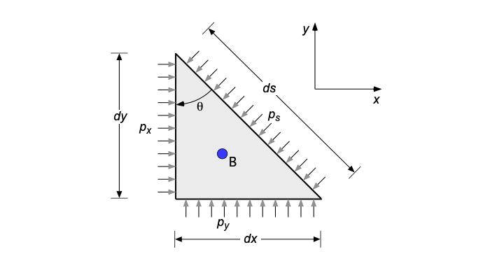](https://eaglepubs.erau.edu/app/uploads/sites/4/2021/07/PascalLaw-3.png)
Schematic used for the derivation of Pascal’s Law in two dimensions; it is easily extended to three dimensions by considering a wedge of fluid.
The pressures acting on the respective faces are  in the \-direction,  in the \-direction, and  along the diagonal. Therefore, for horizontal pressure force equilibrium on the fluid per unit length (i.e., 1 unit into the page), then
(1) 
For the vertical pressure force equilibrium per unit length, then
(2) 
where  is the weight of the fluid per unit length, i.e.,
(3) 
From the geometry of the triangle in Figure 1,  and . Also, as the triangle shrinks to point B in the fluid, but such that  and  become of  in accordance with the continuum assumption, then the product  becomes negligible, i.e., the effects of the weight of fluid inside can be neglected. So, it becomes apparent that
(4) 
and
(5) 
Therefore, from these two latter equations, the conclusion reached is that as the triangle shrinks to point B, then
(6) 
which states that the pressure at any point in a fluid at rest is the same in all directions, as illustrated in Figure 2; this principle is known as *Pascal’s Law*. This latter derivation generalizes easily to three dimensions, showing that .
[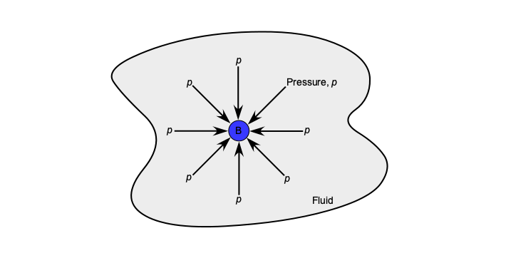](https://eaglepubs.erau.edu/app/uploads/sites/4/2021/07/PascalLaw_point-2.png)
Pascal’s Law states that the pressure at a point is constant and acts equally in all directions; i.e., it is a scalar quantity.
# Aerostatic/Hydrostatic Pressure Field
Remember that pressure is a point property and can vary from point to point within the fluid. With the concept of pressure already discussed, the formal derivation of the equations for the pressure variation in a stagnant fluid can now proceed, and with a particular case of these equations, known as the *aero-hydrostatic equation*. Consider in the differential sense an infinitesimally small volume of fluid in a stagnant flow, i.e., a fluid element of volume , as shown in Figure 3. As the volume becomes infinitesimally small in the limit, it shrinks to point B such that  in accordance with the continuum assumption.
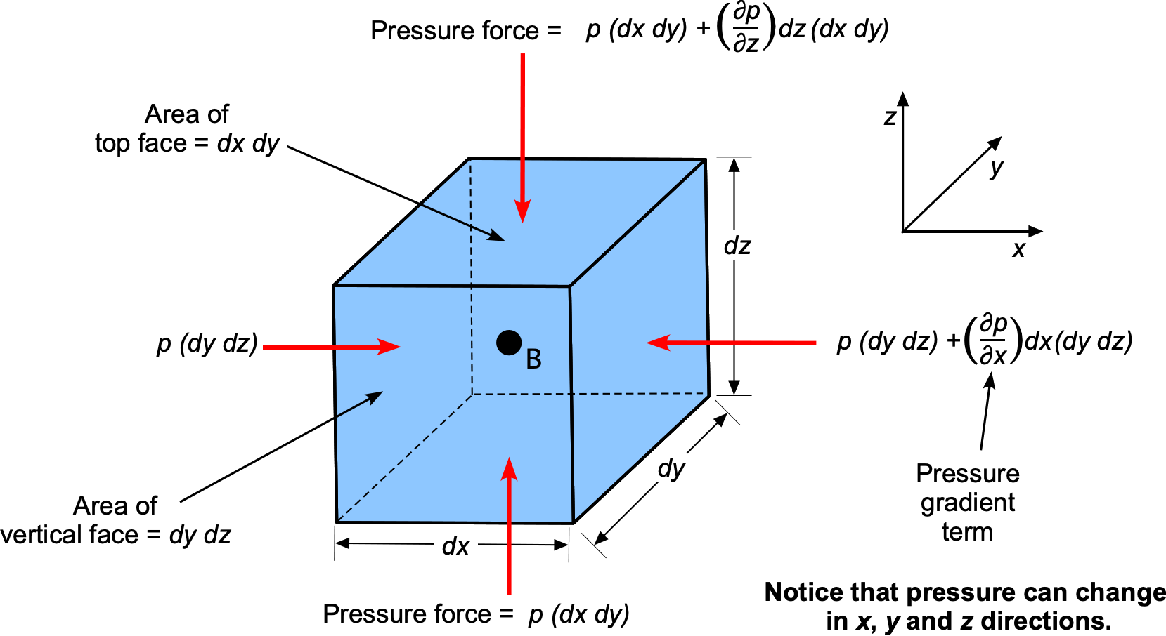
Pressure forces acting on an infinitesimally small, stationary fluid volume with pressure gradients in three directions.
Acting on this small fluid volume are:
1. Pressure forces from the surrounding fluid act normal to the surfaces and vary from point to point, i.e., .
2. Body forces, in general, which are usually expressed as *per unit mas*s of fluid, i.e.,  per unit mass, where the mass in this case is .
3. A specific body force, in the form of gravity, manifests as a vertically downward force because of the weight of the fluid inside the element. This gravitational force can be written as  per unit mass of fluid; the negative sign indicates that the gravitational force acts downward.
**Units of body force per unit mass**
Notice that the units of a body force per unit mass have dimensions of acceleration, i.e., force per unit mass = force/mass = acceleration, so they have units of length/time². Therefore, body forces can also arise from the fluid’s inertial acceleration. For example, even when there is no relative motion between the fluid particles, the entire fluid mass can still be subjected to accelerations. While fluid forces from electromagnetic or electrostatic effects are not a consideration for air, certain types of fluids have properties that respond to such fields and may be explicitly selected for that purpose.
Consider the pressure forces in the  direction, i.e., on the – face of area . Let  be the change of pressure  with respect to . Notice that the partial derivative must be used because the pressure could vary in all three spatial directions. The net pressure force in the  direction is
(7) 
Similarly, for the  direction, the net pressure force is
(8) 
and in the  direction, the net pressure force is
(9) 
Therefore, the net resultant pressure force on the fluid element is
(10) ![\\begin{eqnarray\*} d\\vec{F} & = & dF\_x \\, \\vec{i} + dF\_y \\, \\vec{j} + dF\_z \\, \\vec{k} \\\\\[6pt\] & = & -\\left( \\frac{\\partial p}{\\partial x} \\, \\vec{i} + \\frac{\\partial p}{\\partial y} \\, \\vec{j} + \\frac{\\partial p}{\\partial z} \\, \\vec{k} \\right) dx \\, dy \\, dz \\nonumber \\\\\[6pt\] & = & -\\nabla p \\, (dx \\, dy \\, dz ) = -\\nabla p \\, d {\\mathcal{V}} \\end{eqnarray\*}](https://eaglepubs.erau.edu/app/uploads/quicklatex/quicklatex.com-37f363bbf9677eb1ca31ca88822ff520_l3.svg)
where the [gradient vector operator](https://en.wikipedia.org/wiki/Gradient)  (i.e., “del” or “grad”) has now been introduced.
If  is the mean density of the fluid element, then the total mass of the fluid element, , is , as shown in Figure 4. Any coordinate system can be assumed, but  is usually defined as positive in the vertical direction, where the gravitational acceleration would be . As such, gravity manifests as a vertically downward force from the weight of fluid inside the element, i.e., the net gravitational force is .
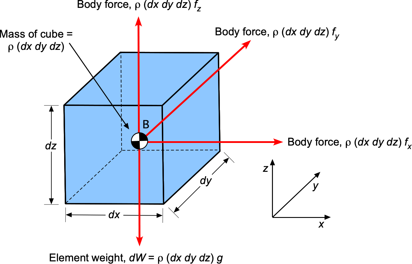
Body forces per unit mass acting on a fluid can include inertial acceleration and gravitational acceleration (i.e., weight).
Furthermore, any additional body forces per unit mass acting on the element can be described as
(11) 
Now, if a fluid element is at rest and in equilibrium, then the sum of the pressure forces, the gravitational force, and the body force must be zero, i.e.,
(12) 
or
(13) 
In scalar form, the preceding vector equation can be written as
(14) ![\\begin{eqnarray\*} \\frac{\\partial p}{\\partial x} & = & \\varrho \\, f\_x \\nonumber \\\\\[6pt\] \\frac{\\partial p}{\\partial y} & = & \\varrho \\, f\_y \\nonumber \\\\\[6pt\] \\frac{\\partial p}{\\partial z} & = & \\varrho \\, f\_z -\\varrho \\, g \\nonumber \\end{eqnarray\*}](https://eaglepubs.erau.edu/app/uploads/quicklatex/quicklatex.com-bce4f73c7237dc8b969fa78dfa8b3075_l3.svg)
Therefore, these three partial differential equations describe the pressure variations within a stagnant fluid. Notice that the center of gravity is at the centroid of the fluid element, so no gravitational moments are acting on the element.
# Effects of Gravity Alone
If the only body force is the effects of gravitational acceleration or gravity force (the weight) acting on the element, then
(15) 
where  is the acceleration under gravity. Gravity manifests as a *downward* force, so there is a minus sign in the  direction, i.e., it is downward because  is measured positively upward. Therefore, in this case
(16) 
or in scalar form
(17) ![\\begin{eqnarray\*} \\frac{\\partial p}{\\partial x} & = & 0 \\nonumber \\\\\[6pt\] \\frac{\\partial p}{\\partial y} & = & 0 \\nonumber \\\\\[6pt\] \\frac{\\partial p}{\\partial z} & = & -\\varrho \\, g \\nonumber \\\\ \\end{eqnarray\*}](https://eaglepubs.erau.edu/app/uploads/quicklatex/quicklatex.com-93e757a1916855c4747cc95704bb88fa_l3.svg)
Because the pressure does not depend on  or , the above equation can now be written as
the ordinary differential equation
(18) 
This differential equation is known as the *hydrostatic equation* or the aero-hydrostatic equation. The aero-hydrostatic equation relates the change in pressure  in a fluid to a change in vertical height . Equation [18](https://eaglepubs.erau.edu/introductiontoaerospaceflightvehicles/chapter/fluid-statics/#id744541393) has numerous applications in manometry, hydrodynamics, and atmospheric physics, including the derivation of the properties of the International Standard Atmosphere (ISA), which is discussed later.
# Solutions to the Aero-Hydrostatic Equation
Several special cases of interest lead to helpful solutions to the aero-hydrostatic equation, namely the pressure changes for:
1. A constant-density fluid, e.g., a liquid.
2. A constant-temperature (isothermal) gas.
3. A linear temperature gradient in a gas.
In the case of gases, once the pressure is known, the corresponding density and/or temperature of the gas can also be solved using the equation of state, i.e.,
(19) 
Remember that the equation of state relates the pressure, , density, , and temperature, , of a gas. If one of these quantities is unknown, the values of the other two can be used to determine it. In the case of liquids, there is no equivalent equation of state because they are incompressible, and their density is constant.
## Isodensity Fluid
If a fluid’s density is assumed to be a constant, e.g., a liquid, then Eq. [18](https://eaglepubs.erau.edu/introductiontoaerospaceflightvehicles/chapter/fluid-statics/#id744541393) can be easily integrated from one height to another to find the corresponding change in pressure. Separating the variables gives
(20) 
and so
(21) 
or
(22) 
This result also means that
(23) 
or perhaps in a more familiar form, as
(24) 
where  is “height.” This simple equation has many applications in various forms of manometry, but it is limited to incompressible fluids, specifically liquids.
![\\\[ \\\]](https://eaglepubs.erau.edu/app/uploads/quicklatex/quicklatex.com-a49807391fa387510b42a56d0d5e0d98_l3.svg)
## Isothermal Gas
If the temperature of a gas is assumed to be constant, i.e., what is known as an isothermal condition, then  constant. In this case, then
(25) ![\\begin{eqnarray\*} \\frac{dp}{dz} & = & -\\varrho \\, g \\\\\[8pt\] T & = & T\_0 \\\\\[8pt\] p & = & \\varrho \\, R \\, T \\end{eqnarray\*}](https://eaglepubs.erau.edu/app/uploads/quicklatex/quicklatex.com-30b5196847836aa3427a66e155e864b6_l3.svg)
By substituting for  and assuming isothermal conditions, then
(26) 
Integrating from  to  where the pressures are  and , respectively, gives
(27) 
Performing the integration gives
(28) 
Therefore,
(29) 
Notice also that for isothermal conditions
(30) 
![\\\[ \\\]](https://eaglepubs.erau.edu/app/uploads/quicklatex/quicklatex.com-a49807391fa387510b42a56d0d5e0d98_l3.svg)
## Linear Temperature Gradient in a Gas
If the temperature of a gas decreases linearly with height, i.e.,  where  is the thermal gradient or “lapse rate,” then in this case
(31) ![\\begin{eqnarray\*} \\frac{dp}{dz} & = & -\\varrho \\, g \\\\\[6pt\] T & = & T\_0 - \\alpha \\, z \\\\\[6pt\] p & = & \\varrho \\, R \\, T \\end{eqnarray\*}](https://eaglepubs.erau.edu/app/uploads/quicklatex/quicklatex.com-e907984dde80e274bd4f64d77c50474e_l3.svg)
Substituting the other two equations into the differential equation gives
(32) 
which is the governing equation that must now be solved. By means of separation of variables and integrating from  to  where the pressures are  and , respectively, gives
(33) 
Performing the integration gives for the left-hand side
(34) 
and for the right-hand side
(35) 
and so the final solution is
(36) 
The corresponding density ratio is
(37) 
# Hydrostatic Paradox
Consider the situation depicted in Figure 5, which shows three containers of different shapes filled with the same liquid. What are the pressure values on the container’s bottom in each case? The answer is that the pressures are *equal* because the hydrostatic equation shows that the pressure at a point in a liquid depends only on the height of the liquid directly above it, , and not on the container’s shape.
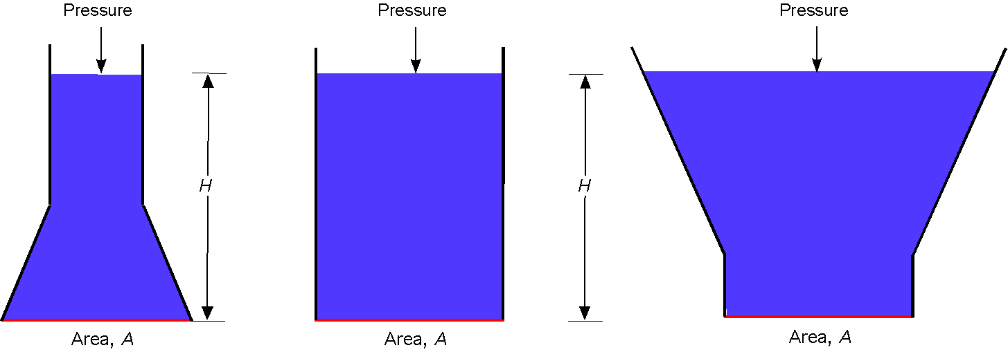
According to the principles of hydrostatics, the pressure at the bottom of each container is the same regardless of its shape or the volume (or weight) of liquid above it.
The pressure at the bottom of each container is , where  is the density of the liquid. If each container has the same bottom area , then the pressure force  on each container’s base is the same. This outcome is independent of the volume of liquid, and the weight of the liquid in each container differs, a phenomenon referred to as the [*hydrostatic paradox*.](https://www.youtube.com/watch?v=J7ymn6f2Bl8)
Check Your Understanding \#1 – Pressure on the bottom of a container
Consider a cylindrical tank containing two liquids of densities  and , as shown in the figure below. Determine an expression for the pressure on the bottom of the tank, . If the heights are  cm and  cm, and the densities are  kg/m and  kg/m. Assume standard atmospheric pressure,  kPa. If the liquids are mixed to form a homogeneous fluid of density , what will be the pressure on the bottom of the tank?[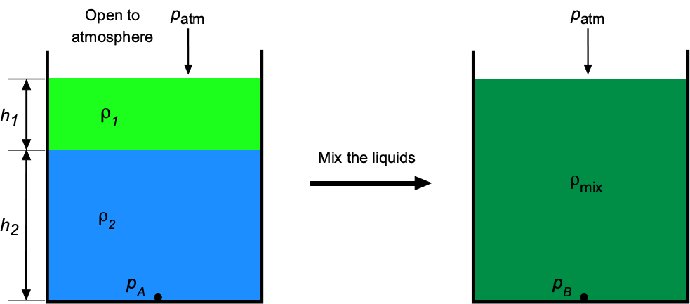](https://eaglepubs.erau.edu/app/uploads/sites/4/2021/07/TwoFluidMixing.png)
Show solution/hide solution.
For the unmixed liquids, the static pressure on the bottom of the tank will be
![\\\[ p\_A = p\_{\\rm atm} + \\varrho\_1 \\, g \\, h\_1 + \\varrho\_2 \\, g \\, h\_2 \\\]](https://eaglepubs.erau.edu/app/uploads/quicklatex/quicklatex.com-aef74defeb653a23db301ae0e40ef0b2_l3.svg)
Inserting the values gives
![\\\[ p\_A = 101.325 \\times 10^3 + 970.0 \\times 9.81 \\times 0.121 + 1,100 \\times 9.81 \\times 0.134 = 103.791\\mbox{kPa} \\\]](https://eaglepubs.erau.edu/app/uploads/quicklatex/quicklatex.com-3b5b6adf5d33c2346076add03fb3c25d_l3.svg)
If the two liquids are homogeneously mixed, then
![\\\[ p\_B = p\_{\\rm atm} + \\varrho\_{\\rm mix} \\, g \\left( h\_1 + h\_2 \\right) \\\]](https://eaglepubs.erau.edu/app/uploads/quicklatex/quicklatex.com-6b5c57e87a223ef332b9964868d02840_l3.svg)
The mixing will not change the net mass of the two liquids, so by conservation of mass, then
![\\\[ M = \\left( \\varrho\_1 \\, g \\, h\_1 + \\varrho\_2 \\, g \\, h\_2 \\right) A = \\varrho\_{\\rm mix} \\, g \\left( h\_1 + h\_2 \\right) A \\\]](https://eaglepubs.erau.edu/app/uploads/quicklatex/quicklatex.com-fbeee7e27e7a76e34ba04167db2d27a8_l3.svg)
where  is the cross-sectional area of the tank. Therefore,
![\\\[ \\varrho\_{\\rm mix} \\, g \\, \\left( h\_1 + h\_2 \\right) = \\left( \\varrho\_1 \\, g \\, h\_1 + \\varrho\_2 \\, g \\, h\_2 \\right) \\\]](https://eaglepubs.erau.edu/app/uploads/quicklatex/quicklatex.com-977496898eed5014023081777f41b415_l3.svg)
Substituting into the expression for  gives
![\\\[ p\_B = p\_{\\rm atm} + \\varrho\_{\\rm mix} \\, g \\left( h\_1 + h\_2 \\right) = p\_{\\rm atm} + \\left( \\varrho\_1 \\, g \\, h\_1 + \\varrho\_2 \\, g \\, h\_2 \\right) = p\_A \\\]](https://eaglepubs.erau.edu/app/uploads/quicklatex/quicklatex.com-d6a703ada0fffbac9dc2d98239c545ae_l3.svg)
Therefore, the pressure at the bottom of the container remains unchanged when the two liquids are mixed.
# Archimedes’ Principle
[Archimedes’ principle](https://en.wikipedia.org/wiki/Archimedes%27_principle) (also spelled Archimedes’s principle) is commonly used to solve hydrostatic problems [\[3\]](https://eaglepubs.erau.edu/introductiontoaerospaceflightvehicles/chapter/fluid-statics/#footnote-194-3 "Archimedes is often considered the father of this field."). This principle states that the upward or *buoyancy force* exerted on a body immersed in a fluid equals the *weight of the fluid* that the body displaces. This outcome occurs whether the body is *wholly or partially submerged* in the fluid, and is independent of its shape. The resulting force also acts upward at the center of buoyancy of the displaced fluid, which is located at the center of mass of the displaced fluid. This principle is commonly applied to problems involving flotation, or the movement of bodies through a fluid, such as boats, ships, balloons, and airships. Balloons and airships are classified as aerostats, or lighter-than-air (LTA) aircraft, in aviation.
## Derivation of Archimedes’ Principle
Having introduced the concept of hydrostatic pressure and the hydrostatic equation, the derivation of Archimedes’ principle is now relatively straightforward because it will be apparent that the source of buoyancy is a consequence of a pressure difference acting on the body. To this end, consider a solid body wholly immersed in a fluid of constant density, as shown in Figure 6. The elemental volume,  has linear dimensions of , , and .
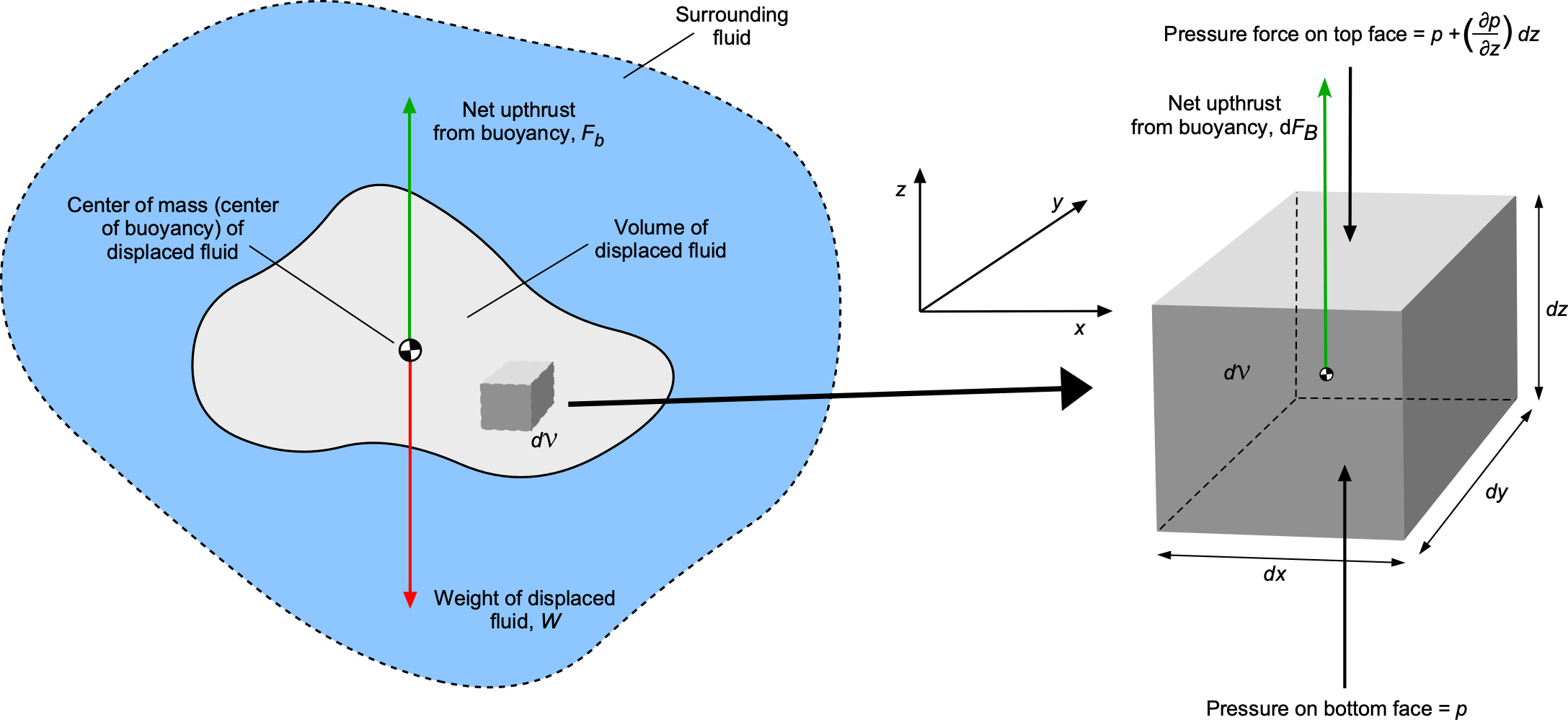
The derivation of Archimedes’ principle requires the hydrostatic equation.
The hydrostatic pressure on the top face of the volume  is lower than that on the bottom face, with the difference providing the upthrust (buoyancy) on the body. It will be apparent that there are no net forces on  in the  and  directions. The net pressure force in the upward  direction, which is the elemental buoyancy force, , will be
(38) 
Using the hydrostatic equation gives
(39) 
Therefore, the buoyancy force on  is
(40) 
Therefore, the total buoyancy force on the immersed body is
(41) 
Because the shape of the body is arbitrary, then
(42) 
which is the net weight of the *fluid* of density  displaced by the volume  of the immersed *body*.
Therefore, the derivation concludes by stating that *the upthrust on the immersed body is equal to the weight of the fluid displaced by the body*, i.e., [Archimedes’ principle](https://archive.org/details/worksofarchimede00arch/page/254/mode/2up?view=theater), which is a consequence of the net difference in hydrostatic pressure force acting on the body. This latter result applies to an immersed body of any shape, including one partially submerged in a fluid.
Check Your Understanding \#2 – Buoyancy force
Which balloon shown in the figure below experiences the most significant buoyancy force? Each balloon contains the same volume of fluid and is surrounded by air.[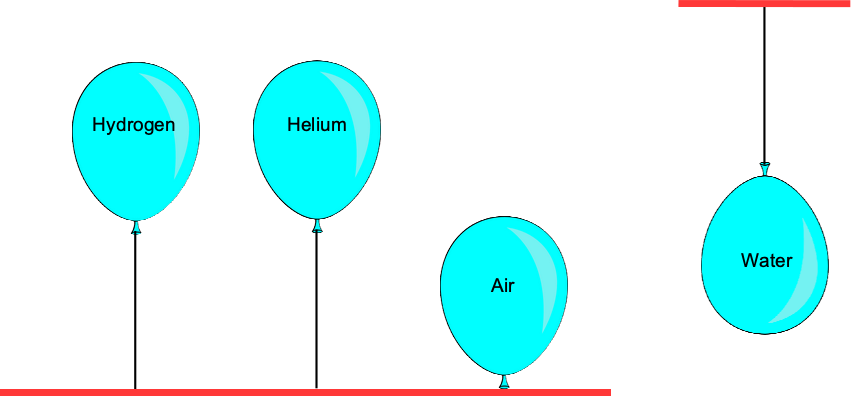](https://eaglepubs.erau.edu/app/uploads/sites/4/2021/07/BalloonBuoyantQuiz.png)
Show solution/hide solution.
The balloons experience the same buoyancy force because each displaces the same volume of air. An assumption is that the water balloon does not stretch with the weight of water. According to Archimedes’ principle, the buoyancy force is equal to the weight of the fluid displaced, not the weight of the fluid inside the balloon. The net upforce, however, does depend on the fluid inside the balloon, so the balloon with the lightest gas (hydrogen) will be the largest. Note: This was not meant to be a trick question.
## Buoyancy & Floatation
To better illustrate the concept of buoyancy, consider the scenarios shown in Figure 7. The object’s volume is the same in each case, but its weight varies from  (heaviest) to  (lightest). If the object is entirely immersed in the fluid, then the upthrust or the buoyancy force, , will be
(43) 
where  is the volume of the object and hence the displaced fluid, and  is the density of the displaced fluid. Remember that the buoyancy force depends on the *weight of the fluid* displaced by the object, not the weight of the object itself.
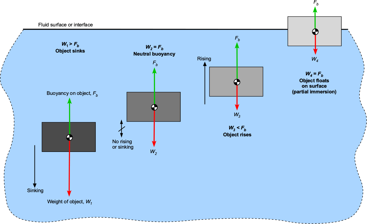
The buoyancy force on an immersed object depends on the weight of the fluid displaced by the object, not the object’s weight. Depending on the net force, a heavy object will sink, and a light object will float.
The net force on the body, therefore, is
(44) 
It will begin to sink if the object is heavier than the buoyancy force, i.e., . If the object has a weight equal to the buoyancy force, i.e., , it will have neutral buoyancy and reach an immersed depth where it will neither sink nor rise in the fluid, i.e., neutral buoyancy like a submarine. The body will begin to rise in the fluid if the buoyancy force exceeds the weight, i.e., . Eventually, if the body is made light enough, it will float at the fluid interface. In this case, only partial immersion may be needed to displace the fluid required to generate the buoyancy force that balances its weight, as in a boat or a ship.
As shown in Figure 8, consider an LTA aircraft suspended in flight. The gas envelope is filled with a lighter gas, called the *buoyant gas*. In the case of the airship, the gas inside will be helium, which is eight times lighter than air. In the case of a balloon, the gas is hot air, which has only a slightly lower density than the surrounding cooler air, depending on the air temperature. In either case, the *upthrust or buoyancy lift force equals the weight of the displaced air.* This upward force is often referred to as *aerostatic* lift because it does not depend on motion.
[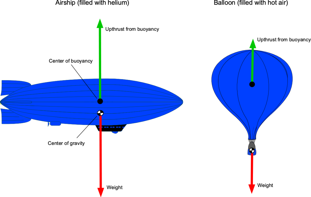](https://eaglepubs.erau.edu/app/uploads/sites/4/2021/07/BuoyancyBalloon-2.png)
The net force acting on an LTA aircraft is equal to the difference between the downward-acting weight of the vehicle and the upward buoyancy force, which is equal to the weight of the displaced air.
The LTA aircraft’s net weight will include the weight of its structure, payload, fuel, and other components, as well as the weight of the gas contained within the gas envelope. Therefore, the net force acting will equal the difference between the net weight of the vehicle minus the weight of the displaced air (i.e., the buoyancy or “upthrust”). If the upthrust exceeds the weight, the aircraft will rise; if it is less, the aircraft will descend. Equilibrium, or neutral buoyancy, will be achieved when these two forces are equal and are in exact vertical balance.
These aerostatic principles can be further developed by using Archimedes’ principle. The net upforce (aerostatic lift), , will be equal to the net weight of the air displaced, less the weight of the gas inside the envelope, i.e., the aerostatic lift is
(45) 
where  is the volume of the envelope containing the buoyant gas,  is the density of the buoyant gas, and  is the density of the displaced air. If the weight of the aircraft is , then for vertical force equilibrium and neutral buoyancy, then
(46) 
Therefore, the volume of the buoyant gas can be determined to provide a specific buoyancy force that overcomes the weight of the object. This is the fundamental principle of aerostatic lift production on all types of LTA aircraft.
Check Your Understanding \#3 – Buoyancy of an airship
An airship has an aerostatic gas envelope with a volumetric capacity of 296,520 ft³, filled with helium. If the airship has an empty weight of 14,188 lb and a maximum fuel load of 960 lb, what would be the maximum payload the airship could carry? Assume MSL ISA standard atmospheric conditions. The density of helium can be assumed to be 0.0003192 slugs/ft3. Ignore the effects of any ballast.
Show solution/hide solution.
The hydrostatic principle of buoyancy is applicable here. Using Archimedes’ principle, the upforce (aerostatic lift), , on the airship will be equal to the net weight of the fluid displaced minus the weight of the gas inside the envelope, i.e.,
![\\\[ L = \\left( \\varrho\_{\\rm air} - \\varrho\_{\\rm He} \\right) g \\, {\\cal{V}} \\\]](https://eaglepubs.erau.edu/app/uploads/quicklatex/quicklatex.com-59dc37554635587519679b86ae0d7293_l3.svg)
where  is the volume of the gas envelope. The gross weight of the airship will be the sum of the empty weight, , plus the fuel weight, , plus the payload, , i.e.,
![\\\[ W = W\_e + W\_f + W\_p \\\]](https://eaglepubs.erau.edu/app/uploads/quicklatex/quicklatex.com-2d06bf818b69de98f2f0969038015d27_l3.svg)
For vertical force equilibrium at takeoff with neutral buoyancy, then , so
![\\\[ W\_e + W\_f + W\_p = \\left( \\varrho\_{\\rm air} - \\varrho\_{\\rm He} \\right) g {\\, \\cal{V}} \\\]](https://eaglepubs.erau.edu/app/uploads/quicklatex/quicklatex.com-604a96d9f06058308a1fcc64c7ced5cb_l3.svg)
Rearranging to solve for the payload weight gives
![\\\[ W\_p = \\left( \\varrho\_{\\rm air} - \\varrho\_{\\rm He} \\right) g \\, {\\cal{V}} - W\_e - W\_f \\\]](https://eaglepubs.erau.edu/app/uploads/quicklatex/quicklatex.com-c9cff517c2c872ed51a399fe11cde08e_l3.svg)
Using the numerical values supplied gives
![\\\[ W\_p = \\left( 0.002378 - 0.0003192 \\right) \\times 32.17 \\times 296,520 - 14,188.0 - 960.0 = 4,497.45~\\mbox{lb} \\\]](https://eaglepubs.erau.edu/app/uploads/quicklatex/quicklatex.com-174a2409d73343c6596431f07b1d4af3_l3.svg)
Therefore, the maximum payload at the takeoff point would be 4,497 lb.
## Horizontal Buoyancy Effects
Horizontal buoyancy occurs whenever pressure gradients are formed and act laterally in a fluid, i.e., in the – plane rather than vertically. In many cases, horizontal pressure gradients arise from inertial accelerations and are prevalent in various aerospace contexts.
For example, flight maneuvers in an airplane produce various inertial “g”- loads that create pressure gradients in fuel tanks, oil reservoirs, and other fluid systems, in addition to vertical gradients. These gradients result in fluid-level variations and sloshing, which must be considered in the design of fluid management systems and during the installation of baffles and vents. Another example is the high acceleration experienced by launch vehicles during flight. During ascent, the vehicle experiences accelerations of 3*–*5*g* in the non-inertial frame fixed to the tank, which appears as a uniform body acceleration in the opposite direction to flight. As the vehicle gains horizontal speed, the effective “gravity” combines with Earth’s gravity to create a steep pressure gradient along and across the tank, pushing the liquid propellant toward the base and the pressurant gas toward the opposite end. These horizontal pressure gradients must be considered in the design of the tank geometry, propellant management devices, and the venting system.
The horizontal buoyancy force on an elemental fluid volume, , that is produced by a pressure gradient in the \-direction is
(47) 
and the corresponding force in the \-direction is
(48) 
In terms of per unit mass , the horizontal buoyancy accelerations are
(49) 
These expressions are the horizontal analog of Archimedes’ principle and the hydrostatic equation.
### Linear Acceleration of the Reference Frame
Suppose the entire coordinate frame accelerates horizontally with constant components  and . In this non-inertial frame, an elemental volume experiences inertial (“fictitious”) forces, i.e.,
(50) 
In terms of per unit mass, then
(51) 
These inertial forces can be written as effective pressure gradients that are identical in form to the buoyancy relations given above, i.e.,
(52) 
### Accelerations in a Rotating Frame
For steady rotation with angular velocity  about the \-axis, a fluid element at radius  experiences an outward specific acceleration  per unit mass. Static equilibrium requires a balancing radial pressure gradient, i.e.,
(53) 
or
(54) 
which integrates to
(55) 
If the fluid is a liquid that has a free surface exposed to atmospheric pressure , using the hydrostatic relation  gives
(56) 
Therefore, the free surface is a paraboloid of revolution with a curvature given by .
Check Your Understanding \#4 – Baffling balloon behavior\!
A helium-filled party balloon tied to a string attached to the seat floats inside a car. If the vehicle accelerates forward, in which direction will the balloon move? If you would like a demonstration, you can use this link: [Baffling Balloon Behavior.](https://www.youtube.com/watch?v=y8mzDvpKzfY) Can you explain the physics of this behavior using the principles of hydrostatics?
[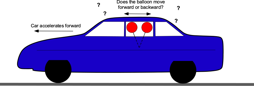](https://eaglepubs.erau.edu/app/uploads/sites/4/2021/07/Car_and_Balloon-2.png)
Show solution/hide solution.
The answer is obtained by using Archimedes’ principle. The net up-force from buoyancy, , on the balloon will be equal to the net weight of the air displaced, less the weight of the helium inside the balloon, as shown in the figure below, i.e.,
![\\\[ L = \\varrho\_{\\rm air} \\, g \\, {\\cal{V}} - \\varrho\_{\\rm He} \\, g \\, {\\cal{V}} = \\left( \\varrho\_{\\rm air} - \\varrho\_{\\rm He} \\right) g \\, {\\cal{V}} \\\]](https://eaglepubs.erau.edu/app/uploads/quicklatex/quicklatex.com-f82f8e37e698c3dc1f3a49e7d1e643f0_l3.svg)
where  is the volume of the balloon,  is the density of air, and  is the density of the helium gas inside the balloon. We are told to neglect the balloon’s weight. Therefore, the tension, , on the string is
![\\\[ T = L = \\left( \\varrho\_{\\rm air} - \\varrho\_{\\rm He} \\right) g \\, {\\cal{V}} \\\]](https://eaglepubs.erau.edu/app/uploads/quicklatex/quicklatex.com-92139a12967b7efb8c8ebbd536242204_l3.svg)
If the car moves forward with a constant acceleration, , in the  direction, then the balance of forces on the balloon will change, as shown in the figure. Because the air mass inside the car is stagnant, the acceleration to the left (in the positive  direction) manifests as an inertial body force on the stagnant air, directed to the right (in the negative  direction). This acceleration will create a horizontal pressure gradient (the higher pressure biased to the rear of the car) that will lead to a net horizontal buoyancy force directed toward the left, i.e.,
![\\\[ F\_x = \\left( \\varrho\_{\\rm air} - \\varrho\_{\\rm He} \\right) a \\, {\\cal{V}} \\\]](https://eaglepubs.erau.edu/app/uploads/quicklatex/quicklatex.com-6afd83e186ad99bf10adacfc2dd8f961_l3.svg)
[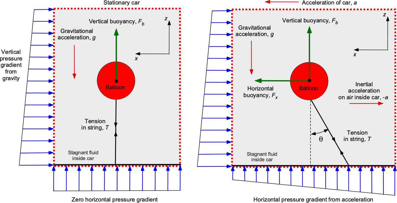](https://eaglepubs.erau.edu/app/uploads/sites/4/2023/10/Balloon_baffling.png)In other words, because of the much lighter helium gas in the balloon, the horizontal buoyancy force in the air is greater than its inertial force. Therefore, it can be concluded that the helium balloon will lean forward relative to the car during acceleration. Finding the angle of the string for horizontal and vertical force equilibrium is just the application of statics, i.e.,
![\\\[ T \\cos \\theta = F\_x \\\]](https://eaglepubs.erau.edu/app/uploads/quicklatex/quicklatex.com-977384759a4af57c666198da4d69014d_l3.svg)
and
![\\\[ T \\sin \\theta = L \\\]](https://eaglepubs.erau.edu/app/uploads/quicklatex/quicklatex.com-f48ceddde189ee456686a13e2375f19e_l3.svg)
Therefore,
![\\\[ \\tan \\theta = \\frac{F\_x}{L} = \\frac{ \\left( \\varrho\_{\\rm air} - \\varrho\_{\\rm He} \\right) a \\, {\\cal{V}}} {\\left( \\varrho\_{\\rm air} - \\varrho\_{\\rm He} \\right) \\, g {\\cal{V}}} = \\frac{a}{g} \\\]](https://eaglepubs.erau.edu/app/uploads/quicklatex/quicklatex.com-59bd87868f5f7bb14204726585605db6_l3.svg)
So, finally, the angle of the string is
![\\\[ \\theta = \\tan^{-1} \\left( \\frac{a}{g} \\right) \\\]](https://eaglepubs.erau.edu/app/uploads/quicklatex/quicklatex.com-7f55caaf0edc7de89af367ea5f2010cc_l3.svg)
# Pressure Forces on Submerged Surfaces
The sum of hydrostatic pressure forces acting on surfaces is a common problem in engineering. Such pressure distributions are typically non-uniform, so the net forces and moments acting on the surface must be obtained by integration. Consider the scenarios shown in Figure 9, which depict the hydrostatic pressure distributions over a vertical flat surface, an inclined flat surface, and a curved surface.
[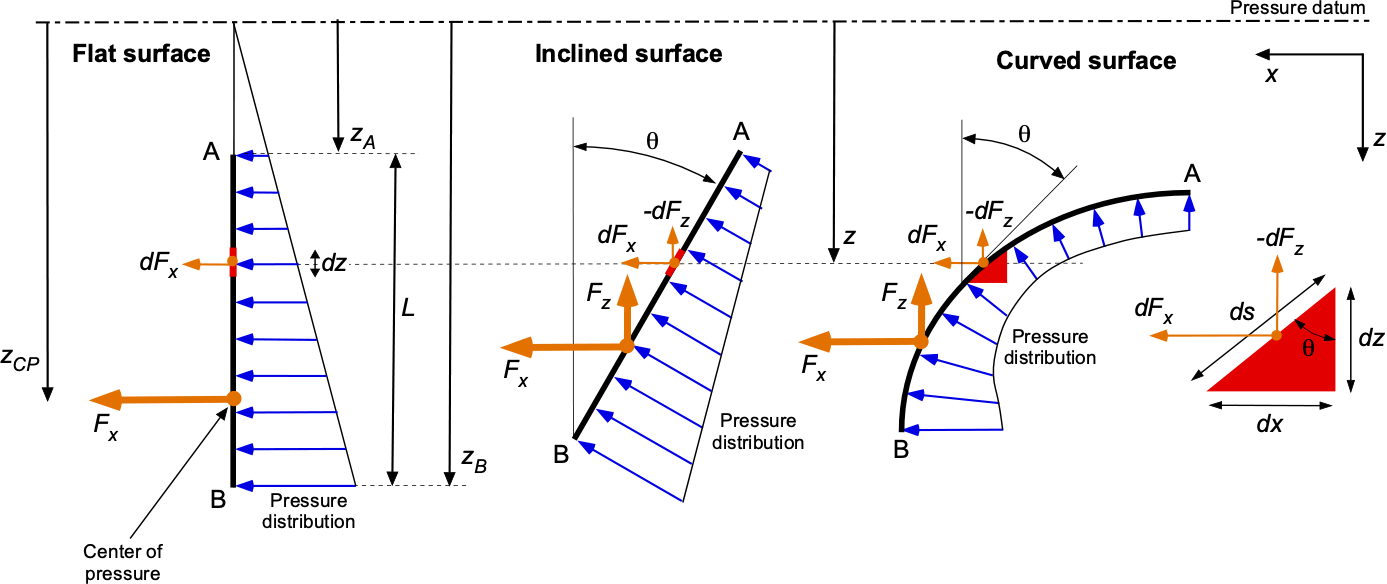](https://eaglepubs.erau.edu/app/uploads/sites/4/2021/07/Pressure_curvedsurface-1.png)
Many engineering problems involve integrating pressure over submerged surfaces in a stagnant fluid, for which hydrostatic principles apply.
## Vertical Flat Surfaces
In the case of the vertical flat surface, the pressure force  acting on the elemental length  at depth  from the pressure datum will be
(57) 
where ‘per unit length’ means 1 unit into the screen or page. The total force acting on the surface will be
(58) 
Performing the integration gives
(59) ![\\begin{equation\*} F\_x = \\varrho \\, g \\left\[ \\frac{z^2}{2} \\right\]\_{z\_A}^{z\_b} = \\varrho \\, g \\left( \\frac{ (z\_A - z\_B)^2 }{2} \\right) = \\varrho \\, g \\left( \\frac{L^2}{2} \\right) \\quad \\mbox{per unit length} \\end{equation\*}](https://eaglepubs.erau.edu/app/uploads/quicklatex/quicklatex.com-73033cbf6da1eef440dc52eb5deea552_l3.svg)
The center of pressure on the plate can be found by taking moments about the pressure datum, i.e.,
(60) 
Performing the integration gives
(61) ![\\begin{equation\*} M = \\varrho \\, g \\left\[ \\frac{z^3}{3} \\right\]\_{z\_2}^{z\_1} = \\varrho \\, g \\left( \\frac{(z\_2 - z\_1)^3}{3} \\right) = \\varrho \\, g \\left( \\frac{L^3}{3} \\right) \\quad \\mbox{per unit length} \\end{equation\*}](https://eaglepubs.erau.edu/app/uploads/quicklatex/quicklatex.com-ecdd8351349be8ef43d49cdb0d384c0f_l3.svg)
Therefore, the center of pressure (cp) will be at
(62) 
which is located at 2/3 of the plate’s length below point A.
## Inclined Flat Surfaces
In the case of an inclined flat surface, the pressure forces per unit length (or span) acting on the elemental length  at depth  from the pressure datum will be
(63) ![\\begin{eqnarray\*} dF\_x & = & \\varrho \\, g \\, z \\, \\sin \\theta \\, dz\\\\\[6pt\] -dF\_z & = & \\varrho \\, g \\, z \\, \\cos \\theta \\, dz \\end{eqnarray\*}](https://eaglepubs.erau.edu/app/uploads/quicklatex/quicklatex.com-3a61cfb814c5b2c9b152f0807e4654f4_l3.svg)
The total force components acting on the surface will be
(64) ![\\begin{eqnarray\*} F\_x & = & \\varrho \\, g \\sin \\theta \\int\_{z\_A}^{z\_B} z \\, dz \\\\\[6pt\] -F\_z & = & \\varrho \\, g \\cos \\theta \\int\_{z\_A}^{z\_B} z \\, dz \\end{eqnarray\*}](https://eaglepubs.erau.edu/app/uploads/quicklatex/quicklatex.com-b356ae0ca284c6babfcab627c2a3c45e_l3.svg)
The  and  terms are taken outside the integral because  is a constant. Performing the integration gives
(65) ![\\begin{eqnarray\*} F\_x & = & \\varrho \\, g \\sin \\theta \\left( \\frac{L^2}{2} \\right) \\\\\[6pt\] -F\_z & = & \\varrho \\, g \\cos \\theta \\left( \\frac{L^2}{2} \\right) \\end{eqnarray\*}](https://eaglepubs.erau.edu/app/uploads/quicklatex/quicklatex.com-43bae82b41a68560dd8aa63e75bffea2_l3.svg)
The center of pressure (cp) on the plate (assume two-dimensional) can be found by taking moments about the pressure datum, as done previously, which in this case is
(66) 
The process can be extended for plates at any orientation in three-dimensional space.
## Curved Surfaces
In the cases of curved surfaces, there are only exact solutions if the geometry lends itself to such, i.e., circular arcs. In this case, the angle terms must be held with the integral such that the total force components acting on the surface will be
(67) ![\\begin{eqnarray\*} F\_x & = & \\varrho \\, g \\int\_{z\_A}^{z\_B} z \\, dx = \\varrho \\, g \\int\_{z\_A}^{z\_B} z \\sin \\theta \\, dz \\\\\[6pt\] -F\_z & = & \\varrho \\, g \\int\_{z\_A}^{z\_B} z \\, dy = \\varrho \\, g \\int\_{z\_A}^{z\_B} z \\cos \\theta \\, dz \\end{eqnarray\*}](https://eaglepubs.erau.edu/app/uploads/quicklatex/quicklatex.com-b7cc18f2018e23b92cdb178e66e9eef7_l3.svg)
The net force is, therefore,
(68) 
Another approach is to perform the integration using the surface expressed in terms of its unit normal vectors, , i.e.,
(69) 
Check Your Understanding \#5 – Moment on a submerged gate
The figure below illustrates that a heavy swinging gate functions as an overpressure release valve. The gate is  = 2 m long and  = 4 m wide. Assume the gate can pivot freely about the hinge and that there is a suitable gasket along its edges to keep it watertight. The water is in a large tank connected to the gate via a channel with a height of  = 0.5 m. The gate must open if the height of the water, , exceeds 5 m.
[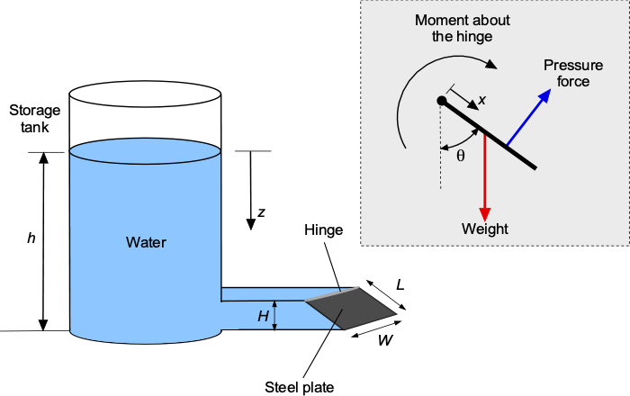](https://eaglepubs.erau.edu/app/uploads/sites/4/2021/07/PressureReleaseGate.png)Determine the equation describing the hydrostatic pressure force on the gate. Find the resultant moment ( torque) about the hinge from the action of the hydrostatic pressure on the gate. What thickness would be needed if the gate is made of solid plate steel (density = 7.5 grams/cm)? Assume that the effects of air pressure on the gate can be neglected compared to the effects of water and that the density of water is  = 1,000 kg/m.
Show solution/hide solution.
The hydrostatic pressure is a linear function of depth , i.e., . Because the gate is at an angle, , to the vertical, the pressure force on the gate will depend on this angle. The lengths  and  are related by , where  = 0.5/2.0 = 0.25, so the angle  is 75.5.
The hydrostatic pressure distribution acting over the gate along its length, , from the hinge will be
![\\\[ p = \\varrho\_w g \\big( (h - H) + x \\cos \\theta \\big) \\\]](https://eaglepubs.erau.edu/app/uploads/quicklatex/quicklatex.com-eb49ff1b21e85b79d8a5e90972a0f698_l3.svg)
The incremental hydrostatic force  on a short width (strip) of the gate  will be
![\\\[ dF\_h = p W dx = \\varrho\_w g \\big( (h - H) + x \\cos \\theta \\big) W \\, dx \\\]](https://eaglepubs.erau.edu/app/uploads/quicklatex/quicklatex.com-77735c967e2c3af90bf23dff39502a3f_l3.svg)
and the corresponding incremental moment (or torque)  about the hinge will be
![\\\[ dM\_h= dF\_h \\, x = \\varrho\_w g \\, W \\big( (h - H) x + \\cos \\theta \\, x^2 \\big) \\, dx \\\]](https://eaglepubs.erau.edu/app/uploads/quicklatex/quicklatex.com-0032acc84e7f713b86e9b5f1585ff7b5_l3.svg)
Therefore, the total hydrostatic moment (or torque)  about the hinge will be
![\\\[ M\_h = \\int\_0^L \\varrho\_w g \\, W \\big( (h - H)x + \\cos \\theta \\, x^2 \\big) \\, dx \\\]](https://eaglepubs.erau.edu/app/uploads/quicklatex/quicklatex.com-819774ffb0628b90b6b4b5a3a3072be3_l3.svg)
which, after integration, becomes
![\\\[ M\_h = \\varrho\_w g \\, W \\bigg\[ \\frac{(h - H) x^2}{2} + \\frac{\\cos \\theta \\, x^3}{3} \\bigg\]\_{0}^{L} \\\]](https://eaglepubs.erau.edu/app/uploads/quicklatex/quicklatex.com-c825ebad039c653794a550189efa47a7_l3.svg)
and so
![\\\[ M\_h = \\varrho\_w g W \\bigg( \\frac{(h - H) L^2}{2} + \\frac{\\cos \\theta \\, L^3}{3} \\bigg) \\\]](https://eaglepubs.erau.edu/app/uploads/quicklatex/quicklatex.com-cb15ebf45a941fccf69f432621a9e84b_l3.svg)
Substituting values gives
![\\\[ M\_h = 1,000 \\times 9.81 \\times 4.0 \\bigg( \\frac{(10.0 - 0.5) 2.0^2}{2} + \\frac{0.25 \\times 2.0^3}{3} \\bigg) = 771.73~\\mbox{kNm} \\\]](https://eaglepubs.erau.edu/app/uploads/quicklatex/quicklatex.com-3937f481b6f698e120136a2fcb47bd36_l3.svg)
The weight  of the steel gate will be
![\\\[ W\_s = \\varrho\_s L \\, W \\, t \\, g \\\]](https://eaglepubs.erau.edu/app/uploads/quicklatex/quicklatex.com-edfd59bb1f3f0c7deddd50e60304d95a_l3.svg)
where  is the thickness of the plate. So, the gravity moment of the plate about the hinge will be
![\\\[ M\_s = W\_s \\left( \\frac{L}{2} \\right) \\sin \\theta = \\varrho\_{s} L \\, W \\ t \\ g \\left( \\frac{L}{2} \\right) \\sin \\theta \\\]](https://eaglepubs.erau.edu/app/uploads/quicklatex/quicklatex.com-70f957883fb0d25a7750ee50400f45bb_l3.svg)
If everything is just in a moment balance, then , so the needed thickness of the plate is
![\\\[ t = \\frac{M\_h}{\\varrho\_s L \\, W \\, g \\displaystyle{\\left( \\frac{L}{2} \\right)} \\sin \\theta} \\\]](https://eaglepubs.erau.edu/app/uploads/quicklatex/quicklatex.com-0aead8c86bfe8fe5702f6e8807e6605e_l3.svg)
The density of steel is 7.5 grams/cm = 7,500 kg/m. Also,  = 0.968. So, after substituting the numerical values, then
![\\\[ t = \\frac{771,730}{7,500 \\times 2.0 \\times 4.0 \\times 9.81\\displaystyle{\\left( \\frac{2.0}{2} \\right)} 0.968} = 1.35~\\mbox{m} \\\]](https://eaglepubs.erau.edu/app/uploads/quicklatex/quicklatex.com-8e5134f2549251b4f1b7116b0a2918bd_l3.svg)
So, a very heavy, thick steel gate is needed.
# Piezometer Tube
A piezometer tube is a simple device used to measure the static pressure of a fluid at a specific point in a pipe, tube, duct, or similar conduit. Its operation is based on the principle that the pressure at a point in a fluid is proportional to the height of the fluid column above that point, as shown in Figure 10.
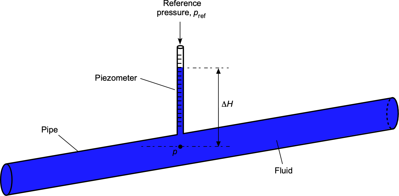
A piezometer is a simple device that measures pressure as a hydrostatic head.
The piezometer height can be used to calculate the pressure head (also known as the piezometric head) at the measurement point. The pressure head, , is the difference between the external reference pressure, , and the pressure in the fluid, , and is given by
(70) 
where  would usually be atmospheric (ambient) pressure, i.e., . The reading is therefore referred to as gauge (or gage) pressure. Piezometers are the simplest type of pressure measurement device. They work with both stagnant (stationary) and flowing fluids. Today, piezometers come in [various types](https://www.encardio.com/blog/what-are-the-different-types-of-piezometers), including solid-state versions.
# U-Tube Manometer
A *U-tube manometer* is the oldest and most basic type of pressure-measuring instrument, and it remains in use today as a reference instrument because of its inherent accuracy. A U-tube manometer is simply a glass tube with a “U” partially filled with a liquid, as shown in Figure 11. This liquid, often referred to as the *manometric liquid*, may be water, alcohol, oil, mercury (rarely used today), or some other liquid of *known* density. Lighter manometric liquids, such as water, are used to measure minor pressure differences, whereas heavier liquids are employed for larger pressure differences. This type of manometer has no moving parts and requires no formal calibration, except for an accurate length scale. The scale may be a simple ruler or a more sophisticated vernier scale.
[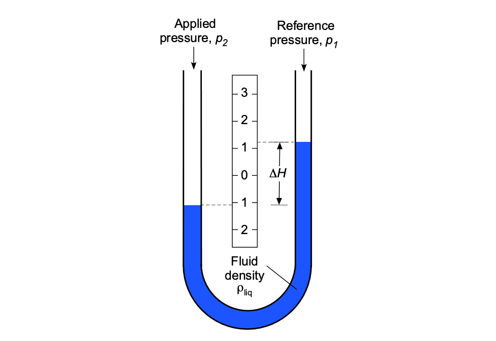](https://eaglepubs.erau.edu/app/uploads/sites/4/2021/07/U-Tube_single.png)
The relative levels of fluid in a U-tube manometer respond to the pressure difference between the two arms of the U-tube.
## Operating Principle
Liquid manometers measure pressure differences by balancing the weight of a manometric liquid between the two applied gas (or air) pressures. The height difference between the liquid levels in the U-tube’s two legs (or arms) is proportional to the air pressure difference; therefore, this height difference can be expressed as a function of the differential pressure.
Using one arm of the manometer as a reference, such as , which could continue to be open to the atmosphere or connected to another (known) reference gas pressure, and connecting the other arm to an unknown applied pressure, m then the difference in the column heights, , is proportional to the difference in the two pressures, i.e.,
(71) 
where  is the density of the manometric liquid used in the U-tube. Notice that a pressure value measured with respect to atmospheric pressure is referred to as *gauge* (or *gage*) pressure. If the reference pressure is a vacuum, the pressure is called *absolute pressure*.
Figure 12 summarizes the changes in liquid levels in a U-tube manometer when the applied air pressure  is greater than, equal to, or less than the reference pressure . For example, if the openings of each arm of a U-tube manometer are exposed to the same pressure, then the heights of the liquid columns will be equal. Increasing the pressure applied to one arm or the other will alter the manometric fluid level.
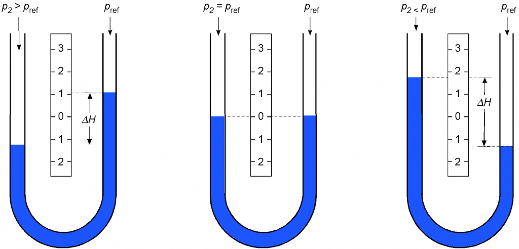
If one arm of a U-tube manometer is exposed to a pressure below atmospheric, the liquid column will rise; if it is exposed to a pressure above atmospheric, the liquid column will fall. If the openings of each arm of a U-tube manometer are exposed to the same pressure, then the heights of the liquid columns will be equal.
Remember that a liquid manometer measures pressure as the difference in height between the manometric fluid columns, typically expressed in inches or centimeters at a specified temperature. The height measurements are easily converted to standard pressure units using appropriate conversion factors, e.g., 1 inch of water equals 5.1971 lb/ft or 0.0361 lb/in.
**“Rules” of Manometry**
Several basic principles or “rules” of manometry directly follow when using the constant density solution to the aero-hydrostatic equation, i.e., p + . Learning to apply these rules properly is achieved by studying exemplar problems in hydrostatics. These rules are:
1. 1. The pressure at two points 1 and 2 in the same fluid at the same height is the same if a continuous line can be drawn through the fluid from point 1 to point 2, i.e.,  =  if  = .
2. Any free surface of a fluid open to the atmosphere is subject to atmospheric pressure, .
3. In most practical hydrostatic problems involving air, atmospheric pressure can be assumed constant at all heights unless the vertical change is significant (e.g., more than a few feet or meters).
4. For a liquid in a container, the shape of the container does not matter in hydrostatics; i.e., the pressure at a point in the liquid depends only on the vertical height of the fluid above that point. This result is called the *hydrostatic paradox.*
5. The pressure is constant across any flat fluid-to-fluid interface.
## Variations of U-tube Manometers
Many variations of the basic U-tube manometer concept include inverted, inclined, and reservoir or well-type manometers. All manometers respond to changes in pressure by vertical changes in fluid height.
### Inverted Manometer
An inverted U-tube manometer is often used to measure pressure differences in liquids; see Figure 13. The space above the liquid in the manometer is filled with air at a known reference pressure, which can be adjusted to balance the liquid levels and adjust the manometer’s sensitivity. When the pressure at B is higher than at A, the liquid in the U-tube is displaced, creating a difference in the liquid levels in the two arms of the tube. The difference in the liquid levels is directly proportional to the pressure difference between the two points, i.e.,
(72) 
[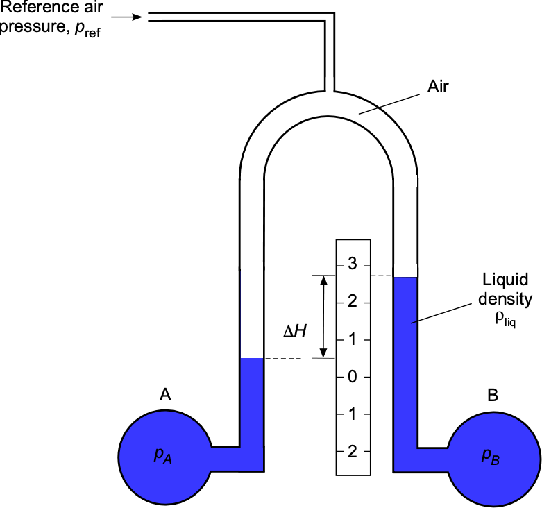](https://eaglepubs.erau.edu/app/uploads/sites/4/2021/07/U-Tube_inverted-1.png)
Inverted U-tube manometers are commonly used to measure pressure differences in liquids.
### Asymmetric Manometers
Asymmetric manometers are sometimes encountered, in which one arm of the manometer has a different cross-sectional area from the other, as shown in Figure 14. The natural question that arises, therefore, is whether the difference in the two fluid levels is the same as that of a symmetric manometer for a given air pressure difference.
[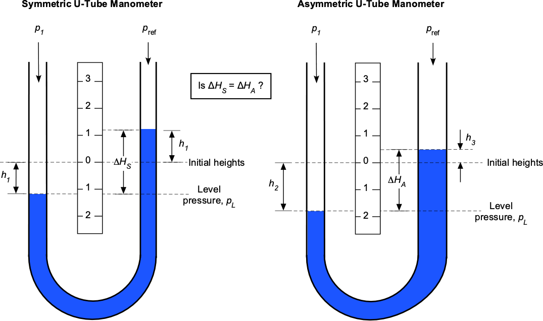](https://eaglepubs.erau.edu/app/uploads/sites/4/2021/07/U-Tube_asymmetric.png)
Symmetric U-tube manometer (left) and asymmetric U-tube manometer (right). Are the values of  and  equal for a given pressure difference?
In the case of the symmetric manometer, it will be apparent that for a given air pressure difference, , the liquid level on the left arm will drop by the same amount, , as the level increases on the right arm, i.e., conservation of mass and volume (both are conserved for a liquid). Therefore, applying hydrostatic principles to the right arm of the symmetric manometer at a level pressure gives
(73) 
ignoring any hydrostatic effects of the air. Applying hydrostatic principles to the left arm of the symmetric manometer, then at the level pressure values
(74) 
where “level pressure” denotes the pressure at the same height in both arms of the manometer. Therefore,
(75) 
In the case of the asymmetric manometer, the liquid level in the right arm will not rise as far as it does in the symmetric manometer. However, to satisfy the conservation of volume, the level in the left arm must drop more, i.e.,  and . Applying hydrostatic principles to the right arm of the asymmetric manometer at the level pressure, then
(76) 
again, ignoring any hydrostatic effects of the air. Applying hydrostatic principles to the left arm of the asymmetric manometer, then
(77) 
as before. Therefore, in this case
(78) 
Finally, equating Eq. [75](https://eaglepubs.erau.edu/introductiontoaerospaceflightvehicles/chapter/fluid-statics/#id2395298169) obtained for the symmetric manometer and Eq. [78](https://eaglepubs.erau.edu/introductiontoaerospaceflightvehicles/chapter/fluid-statics/#id1394858960) for the asymmetric manometer gives
(79) 
proving that  is equal to  for the same . The conclusion is that *regardless of the cross-sectional areas of the arms* of a U-tube manometer, a given applied differential pressure will create the same height *difference* on the liquid levels, even though the levels themselves will be different (conservation of mass or volume) compared to the case where the legs have the same area.
**Level Pressure in Hydrostatics**
In a fluid at rest, the pressure varies only with vertical position. The hydrostatic relation is
![\\\[ \\frac{dp}{dz} = -\\varrho \\, g \\\]](https://eaglepubs.erau.edu/app/uploads/quicklatex/quicklatex.com-5be4ea88602757061e7c778341a1057a_l3.svg)
which shows that pressure decreases with increasing elevation. Consequently, any two points within the same continuous fluid that lie at the same vertical level must have the same pressure. This principle is often referred to as *level pressure*. It states that in a static fluid, the pressure at all points on a horizontal plane is identical. The concept is used extensively in the analysis of manometers. When evaluating a U-tube manometer, the pressures at two points located at the same height within the connected fluid must be equal. By equating the pressures at a reference level, the pressure difference between the two arms can be directly related to the height difference between the fluid columns.
### Well Manometer
The simple U-tube manometer has a significant disadvantage: the liquid levels in both arms must be measured and recorded to determine the pressure. By making the diameter of one arm much larger than the other, the manometric liquid level will fall very slightly on that arm compared to the more significant rise in the other arm. This principle is used in a *well-type* or *reservoir-type* manometer, as shown in Figure 15, which is just another variation of the asymmetric manometer.
[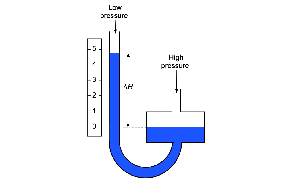](https://eaglepubs.erau.edu/app/uploads/sites/4/2021/07/Well_Manometer.png)
Well-type manometers are often used for reference pressure measurements or calibrations of other pressure-measuring devices.
In this case, the drop in the well’s liquid level can be ignored in practice. The differential pressure can then be obtained in the standard way by measuring the change in the fluid level in the well relative to the vertical height of the column, i.e.,
(80) 
Some well manometers used for high accuracy may require a slight adjustment, as the scale’s datum can be moved to “zero” the reading relative to the well level. In either case, only one reading on the scale is required to determine the differential pressure. Well-type manometers are often used to measure low-pressure differentials or as calibration manometers, but they are not limited to these uses.
### Inclined Manometer
With an inclined manometer arm, as shown in Figure 16, a vertical change in the fluid levels is stretched over a longer length. Consequently, an inclined-arm manometer has better sensitivity for measuring lower pressures, i.e.,
(81) 
This means that the length along the arm is “magnified” according to
(82) 
For example, if  then . Because the fluid level moves further along the arm for a given pressure difference, it is easier to measure on the scale.
[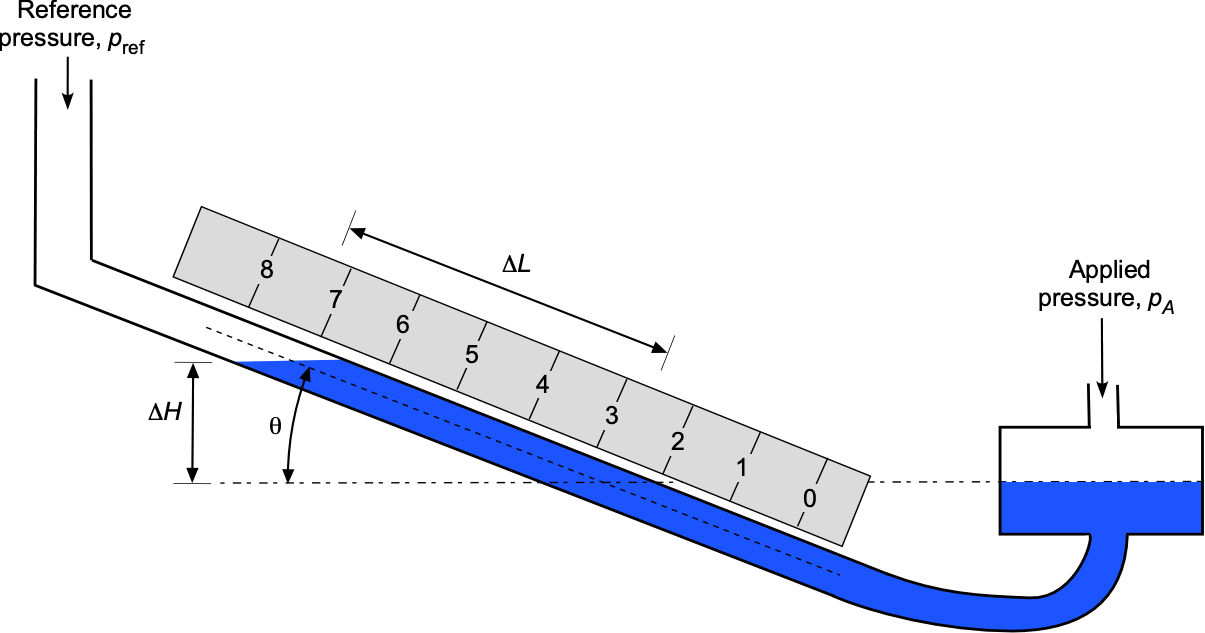](https://eaglepubs.erau.edu/app/uploads/sites/4/2021/07/Inclined_Manometer.png)
An inclined manometer is more sensitive because it causes the liquid in the arm to move more when the applied pressure changes.
### Bank Manometers
Liquid manometers are helpful in many applications, but they have limitations because of their large size, bulkiness, and suitability for laboratory rather than routine field use. They also come in large banks suitable for use in the wind tunnel, as shown in Figure 17. One side of the manometer bank is referenced to static pressure through a plenum containing the manometer liquid (usually water with a dye added), much like a well-type manometer. Each individual manometer is connected to a separate pressure tap, such as on a wing. The process remains the same because the pressure is proportional to the height of the fluid column, which can be measured with a scale. Such manometers, however, require a very long time to read and cannot be interfaced with a computer other than manually.
[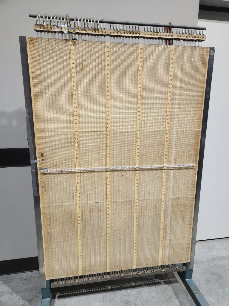](https://eaglepubs.erau.edu/app/uploads/sites/4/2021/07/Manometerstack_ERAU-scaled.jpg)
A liquid-filled manometer bank for use in the wind tunnel, now replaced by solid-state pressure transducers.
Check Your Understanding \#6 – Use of a U-tube manometer
A U-tube manometer is connected to the inlet and outlet of a water pump, as shown in the figure below. The left side is connected to the inlet at pressure , and the right side is connected to the outlet at pressure . Assuming that the inlet and outlet conditions are at the same elevation, determine the pump’s pressure increase. Remember that specific gravity SG = . The density of water can be assumed to be 1.93 slugs/ft.
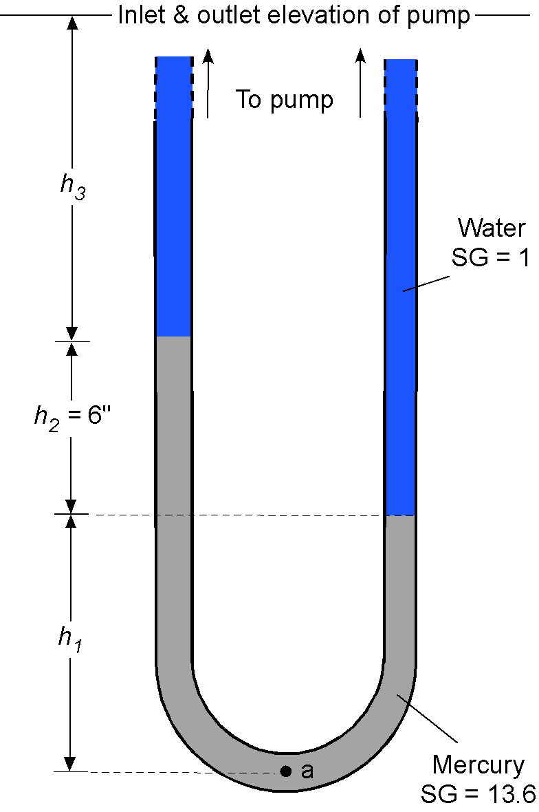
Show solution/hide solution.
The pressure at point “a” will equal the pressure produced by each arm of the U-tube manometer. For the left arm, then
![\\\[ p\_a = \\varrho\_{\\rm Hg} \\, g \\, h\_1 + \\varrho\_{\\rm Hg} \\, g \\, h\_2 + \\varrho\_{\\rm H\_{2}O} \\, g \\, h\_3 + p\_{\\rm in} \\\]](https://eaglepubs.erau.edu/app/uploads/quicklatex/quicklatex.com-7f4d1b2f5b45a744380f0ef0f763117e_l3.svg)
Similarly, for the right arm, then
![\\\[ p\_a = \\varrho\_{\\rm Hg} \\, g \\, h\_1 + \\varrho\_{\\rm H\_{2}O} \\, g \\, h\_2 + \\varrho\_{\\rm H\_{2}O} \\, g \\, h\_3 + p\_{\\rm out} \\\]](https://eaglepubs.erau.edu/app/uploads/quicklatex/quicklatex.com-3ebd162cf15393e10cdae78c5afa71f6_l3.svg)
Therefore, the difference in pressure becomes
![\\\[ \\Delta p = p\_{\\rm out} - p\_{\\rm in} = \\varrho\_{\\rm Hg} \\, g \\, h\_2 - \\varrho\_{\\rm H\_{2}O} \\, g \\, h\_2 = \\left( \\varrho\_{\\rm Hg} - \\varrho\_{\\rm H\_{2}O} \\right) g \\, h\_2 \\\]](https://eaglepubs.erau.edu/app/uploads/quicklatex/quicklatex.com-93dddaaa488936ab0d4fcfc35e4a6176_l3.svg)
or
![\\\[ \\Delta p = \\left( SG\_{\\rm Hg} - SG\_{\\rm H\_{2}O} ) \\varrho\_{\\rm H\_{2}O} \\right) g \\, h\_2 \\\]](https://eaglepubs.erau.edu/app/uploads/quicklatex/quicklatex.com-c6400e6a4d05ea23d24f5349c457e160_l3.svg)
Substituting the known numerical values gives
![\\\[ \\Delta p = \\left( 13.6 - 1.0 \\right) \\times 1.93 \\times 32.17 \\times (6.0/12) = 391.16~\\mbox{lb/ft\${^{2}}\$} \\\]](https://eaglepubs.erau.edu/app/uploads/quicklatex/quicklatex.com-fc580f2aafd97d4093e2da2fe72f60ac_l3.svg)
# Pressure Transducers
The schematic below illustrates that a pressure sensor or pressure transducer is a solid-state device used for measuring pressure. A pressure sensor generates a voltage or other analog signal that is a function of the pressure imposed upon it. The sensor must be calibrated by applying known pressures and recording the output voltage; the resulting relationship is known as the *calibration function*. This relationship is typically linear, as illustrated in Figure 18, so a single constant, or *calibration coefficient*, represents the behavior. The sensor’s signal may also be amplified and filtered, then converted to digital form by an analog-to-digital (A/D) converter before being stored on a computer.
[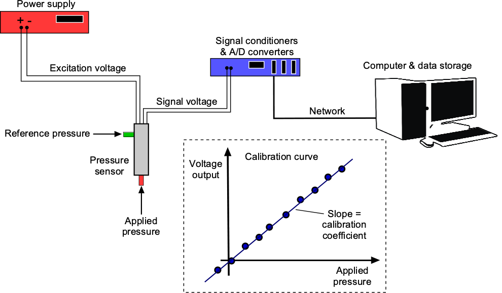](https://eaglepubs.erau.edu/app/uploads/sites/4/2021/07/Pressure_transducer.png)
Pressure transducers measure pressure values as a voltage output. The relationship between pressure and output is obtained through calibration.
Digital pressure manometers are also available in convenient, portable, battery-powered formats for ease of use, with single- or multi-input, multi-output capabilities for controlling measurements and transferring data. In addition, calibrations or correction factors can be incorporated into the software used to manage the digital manometer. Today, pressure sensors are utilized in thousands of industrial applications and are available in various sizes, shapes, and pressure ranges. Miniature pressure transducers are often used in aerospace applications because of their low weight and their ability to be mounted closely together, for example, over the surface of a wing. In wind tunnel applications, pressure transducer modules, such as the one shown in Figure 19, are often used. Pressure tubes can be connected to each port, and the module has self-contained electronics that allow it to read digital pressure values directly from a computer and store them for analysis.
[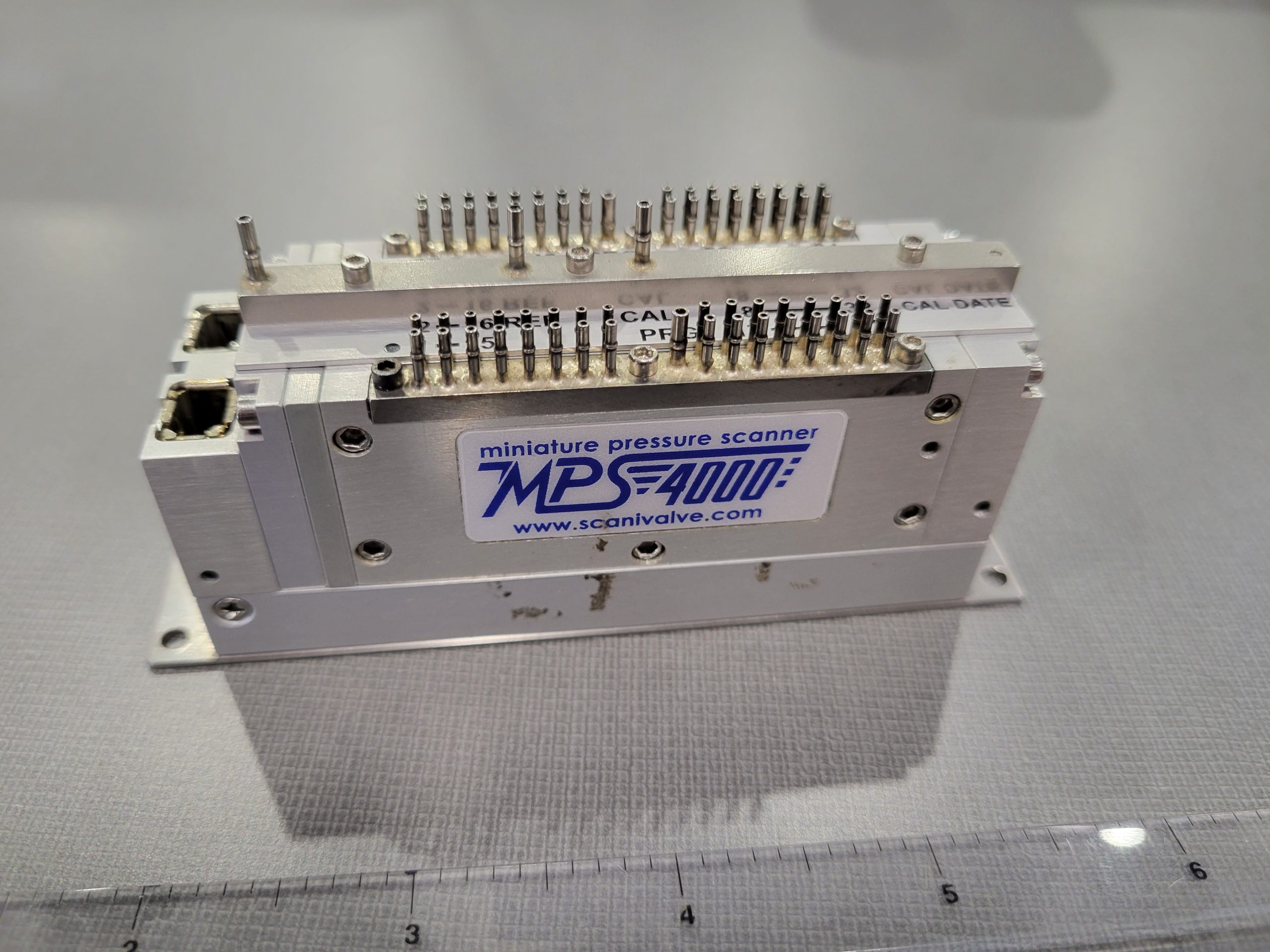](https://eaglepubs.erau.edu/app/uploads/sites/4/2022/07/ScaniValve-scaled-1.jpg)
A miniature solid-state pressure transducer block enables the digital measurement of 64 pressure values at high data rates.
# Hydraulic Press
A *hydraulic press* uses the principles of hydrostatics to amplify a relatively small input force applied to a piston in a primary cylinder into a significantly larger output force applied to a piston in a secondary cylinder. This concept is called *mechanical advantage*. It is widely used in the design of hydraulic systems to generate larger mechanical forces where needed, as shown in Figure 20. This approach can be applied to various tools, machinery, and aircraft components, including landing gear, flaps, flight control surfaces, and brakes.
[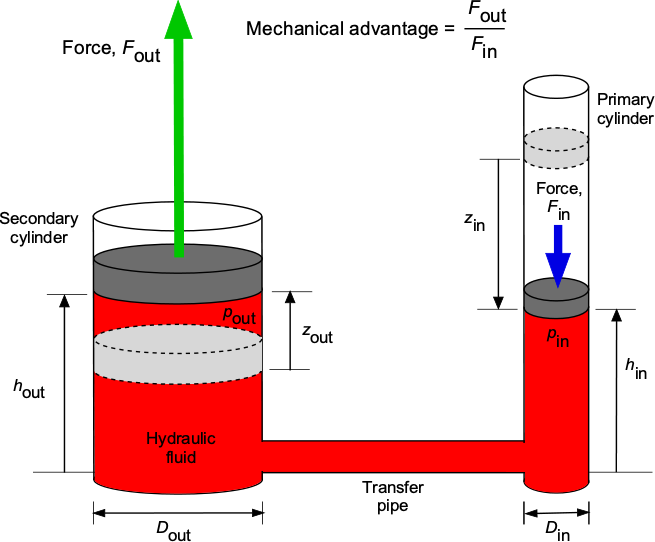](https://eaglepubs.erau.edu/app/uploads/sites/4/2021/07/Piston_hydrauliclift-3.png)
The principle of a hydraulic press is to multiply an applied force to give a mechanical advantage.
The fluid is a form of hydraulic oil, which can be considered incompressible, with a density of . The system comprises two cylinders of different diameters,  and , respectively, each filled with hydraulic fluid and capped with a tight-fitting piston that slides within the cylinder. The applied force, , on the primary piston moves the piston downward, thereby driving the fluid through a transfer pipe into the secondary cylinder. The force on the primary piston also increases the pressure, which is transmitted hydrostatically to the secondary piston, resulting in the exact change in pressure there. The secondary piston has a larger area, thereby producing a greater force, , for the same pressure.
Assume the system is initially in hydraulic equilibrium with no forces acting on either piston. The force  applied to the primary piston moves it down by a distance , increasing the pressure below the piston to
(83) 
On the secondary or output side, the pressure below the piston is
(84) 
Also, it will be apparent that because the pressures at the same height in the same fluid are equal, then
(85) 
Therefore, introducing the pressure values in terms of forces gives
(86) 
or
(87) 
If the difference in hydrostatic pressure head, , can be assumed to be small compared to the pressure applied by the forces, which is easily justified, then , and so
(88) 
This means that the output force on the secondary piston is
(89) 
Therefore, input force, , will be multiplied by the ratio of the areas or the square of the diameter ratios of the primary and secondary cylinders to give a higher output force, . For example, if , then  and so a mechanical advantage of 5.
Notice that the distance the primary piston must move in its cylinder is greater than the distance the secondary piston moves. The volume of fluid shared below the two pistons is conserved (oil is incompressible), i.e.,
(90) 
so that
(91) 
If , then , so the primary piston must move five times as far, which is the price to pay for a mechanical advantage.
The problem can also be addressed using the law of conservation of energy. The work done by the force on the primary piston must appear as work by the secondary piston, assuming no losses in the fluid transfer, i.e.,
(92) 
Therefore, the same result of the multiplication of forces is obtained, i.e.,
(93) 
# Summary & Closure
The principles of hydrostatics apply to stationary or stagnant fluids, i.e., fluids in which there is no relative motion between their elements. Therefore, these fluid problems are easier to understand and predict. Problems that can be analyzed using hydrostatics include buoyancy, the determination of pressures on submerged objects or within fluid-filled containers, and other fluid problems in which the fluid is stationary. In addition to pressure, other fluid properties of interest include temperature and density. The essential equations to remember are those for the hydrostatic pressure field and the aero-hydrostatic equation. The latter is a special case of the former when gravity is the only body force acting. The equation of state is also helpful in analyzing hydrostatic problems and for relating pressures, densities, and temperatures in a gas. Another application of the aero-hydrostatic equation is to analyze the properties of Earth’s atmosphere and those of other planetary atmospheres.
5-Question Self-Assessment Quickquiz
For Further Thought or Discussion
- A balloon filled with helium is released at sea level. What happens to the balloon?
- Can a lead balloon float? Be sure to explain any assumptions you may use.
- A cylindrical container (bucket) filled with water is rotated. What happens to the shape of the water’s surface?
- In a density-stratified water container, the density varies with depth according to  = 1000 + 1.1  for 0 \<  \< 100 m, where  = 0 is the surface. Show how to determine the pressure field.
- Sometimes, an inclined manometer is used to measure pressure. Explain why.
- Explain the principle of a hydraulic lift for obtaining a large force from a small force.
- A cruise ship weighs 100,000 tons. How much volume of seawater does it displace?
- Precision liquid manometers are still used today, which may seem inconvenient, but they are not outdated. Explain why.
- What factors influence the stability of floating objects? How can you determine the equilibrium position of a floating body and its stability conditions?
Additional Online Resources
To improve your understanding of hydrostatics, take some time to navigate to some of these online resources:
- Wikipedia has a good site on [hydrostatics](https://en.wikipedia.org/wiki/Hydrostatics).
- [Video](https://en.wikipedia.org/wiki/Hydrostatics) on the concept of hydrostatic pressure from the University of Colorado.
- [Video](https://en.wikipedia.org/wiki/Hydrostatics) on visualizing the idea of hydrostatic pressure.
- For an interactive demonstration about hot air balloons, see: [How do you control a hot air balloon?](https://www.ck12.org/c/physics/archimedes-law/rwa/Hot-Air-Balloons/)
- For more on Archimedes and his principle, check out [Eureka! The Archimedes Principle](https://www.livescience.com/58839-archimedes-principle.html).
- Pascal’s principle, hydrostatics, atmospheric pressure, lungs, and tires. Good [lecture](https://www.youtube.com/watch?v=O_HQklhIlwQ) and demonstrations.
- Hydrostatics, Archimedes’ Principle: What makes your boat float? Good [lecture](https://www.youtube.com/watch?v=JR-L2CS8DGc) and excellent demonstrations.
***
1. Which may include translational, centrifugal, and Coriolis accelerations. [↵](https://eaglepubs.erau.edu/introductiontoaerospaceflightvehicles/chapter/fluid-statics/#return-footnote-194-1)
2. These forces are significant in conducting fluids, such as plasmas and electrolytes. [↵](https://eaglepubs.erau.edu/introductiontoaerospaceflightvehicles/chapter/fluid-statics/#return-footnote-194-2)
3. Archimedes is often considered the father of this field. [↵](https://eaglepubs.erau.edu/introductiontoaerospaceflightvehicles/chapter/fluid-statics/#return-footnote-194-3)
Previous/next navigation
[Previous: Fundamental Properties of Fluids](https://eaglepubs.erau.edu/introductiontoaerospaceflightvehicles/chapter/fundamental-properties-of-fluids/)
[Next: Atmospheric Properties](https://eaglepubs.erau.edu/introductiontoaerospaceflightvehicles/chapter/international-standard-atmosphere-isa/)
Back to top
## License

[Introduction to Aerospace Flight Vehicles](https://eaglepubs.erau.edu/introductiontoaerospaceflightvehicles) Copyright © 2022–2026 by J. Gordon Leishman is licensed under a [Creative Commons Attribution-NonCommercial-NoDerivatives 4.0 International License](https://creativecommons.org/licenses/by-nc-nd/4.0/), except where otherwise noted.
## Digital Object Identifier (DOI)
<https://doi.org/https://doi.org/10.15394/eaglepub.2022.1066.9>
## Share This Book
[Pressbooks](https://pressbooks.com/)
[Powered by Pressbooks](https://pressbooks.com/)
- [Pressbooks User Guide](https://guide.pressbooks.com/)
- \|[Pressbooks Directory](https://pressbooks.directory/)
- \|[Contact](https://erau.libwizard.com/f/PBContact%20)
[Pressbooks on YouTube](https://www.youtube.com/user/pressbooks)
[Pressbooks on LinkedIn](https://www.linkedin.com/company/pressbooks/?originalSubdomain=ca) | |||||||||
| Readable Markdown | In fluid mechanics, a primary concern is the description and *understanding* of fluid motion, i.e., fluid dynamics. First, note that air is a type of *fluid*, along with gases and liquids. However, if the fluid is not moving, it is commonly referred to as *stagnant*. In that case, its characteristics and properties (e.g., pressure and density) can be described more easily using the principles of *fluid statics*.
A fluid in *static equilibrium* is one in which every fluid particle is either at rest or has no relative motion with respect to the other particles in the fluid. No viscous forces act on stagnant fluids because there is no relative motion between the fluid elements. Under these conditions, two types of forces on the fluid must be considered:
1. Body forces, e.g., weight and inertial accelerations[\[1\]](https://eaglepubs.erau.edu/introductiontoaerospaceflightvehicles/chapter/fluid-statics/#footnote-194-1 "Which may include translational, centrifugal, and Coriolis accelerations."), and possibly electromagnetic forces.[\[2\]](https://eaglepubs.erau.edu/introductiontoaerospaceflightvehicles/chapter/fluid-statics/#footnote-194-2 "These forces are significant in conducting fluids, such as plasmas and electrolytes.")
2. Surface forces, e.g., the effects of an external pressure acting over an area.
The term *hydrostatics* is often used to refer to fluid statics in general*.* Therefore, hydrostatic principles apply to all fluids, both gases and liquids. However, hydrostatic principles are frequently used to analyze liquids and other predominantly incompressible fluids, i.e., fluids that can be assumed to have constant density. The terms *aerostatics* and pneumatics are used when the principles of fluid statics are applied to compressible fluids, such as gases (e.g., air). Examples of engineering problems that could be analyzed by using hydrostatics and aerostatics include the following:
1. The measurement of pressure using various types of manometry.
2. The buoyancy and stability of floating objects, such as ships in the water, and lighter-than-air aircraft, such as balloons and blimps.
3. The pressure and other fluid properties inside containers or vessels, including those caused by body forces or acceleration fields.
4. The properties of the atmosphere on Earth and other planets.
5. The transmission of forces and power using pressurized liquids and/or gases.
- Understand the meaning of a stagnant fluid and the underlying principles that apply to the behavior of static fluids.
- Derive, understand, and use the general equations for an aero-hydrostatic pressure field.
- Understand how to develop and apply the aero-hydrostatic equation.
- Use the principles of hydrostatics and the aero-hydrostatic equation to solve some fundamental engineering problems.
The pressure at a point in a fluid at rest is equal in all directions; therefore, pressure is an isotropic scalar quantity, as formally embodied in [*Pascal’s Law*](https://en.wikipedia.org/wiki/Pascal%27s_law). The derivation of Pascal’s Law proceeds by considering an infinitesimally small right-angled, three-dimensional fluid wedge at rest. However, the outcome is most easily obtained if the wedge is examined in just one view (or one plane), as shown in Figure 1, which appears as a right-angled triangle with horizontal side length , vertical side length , and diagonal length , with the contained angle .
[](https://eaglepubs.erau.edu/app/uploads/sites/4/2021/07/PascalLaw-3.png)
Schematic used for the derivation of Pascal’s Law in two dimensions; it is easily extended to three dimensions by considering a wedge of fluid.
The pressures acting on the respective faces are  in the \-direction,  in the \-direction, and  along the diagonal. Therefore, for horizontal pressure force equilibrium on the fluid per unit length (i.e., 1 unit into the page), then
(1) 
For the vertical pressure force equilibrium per unit length, then
(2) 
where  is the weight of the fluid per unit length, i.e.,
(3) 
From the geometry of the triangle in Figure 1,  and . Also, as the triangle shrinks to point B in the fluid, but such that  and  become of  in accordance with the continuum assumption, then the product  becomes negligible, i.e., the effects of the weight of fluid inside can be neglected. So, it becomes apparent that
(4) 
and
(5) 
Therefore, from these two latter equations, the conclusion reached is that as the triangle shrinks to point B, then
(6) 
which states that the pressure at any point in a fluid at rest is the same in all directions, as illustrated in Figure 2; this principle is known as *Pascal’s Law*. This latter derivation generalizes easily to three dimensions, showing that .
[](https://eaglepubs.erau.edu/app/uploads/sites/4/2021/07/PascalLaw_point-2.png)
Pascal’s Law states that the pressure at a point is constant and acts equally in all directions; i.e., it is a scalar quantity.
Remember that pressure is a point property and can vary from point to point within the fluid. With the concept of pressure already discussed, the formal derivation of the equations for the pressure variation in a stagnant fluid can now proceed, and with a particular case of these equations, known as the *aero-hydrostatic equation*. Consider in the differential sense an infinitesimally small volume of fluid in a stagnant flow, i.e., a fluid element of volume , as shown in Figure 3. As the volume becomes infinitesimally small in the limit, it shrinks to point B such that  in accordance with the continuum assumption.

Pressure forces acting on an infinitesimally small, stationary fluid volume with pressure gradients in three directions.
Acting on this small fluid volume are:
1. Pressure forces from the surrounding fluid act normal to the surfaces and vary from point to point, i.e., .
2. Body forces, in general, which are usually expressed as *per unit mas*s of fluid, i.e.,  per unit mass, where the mass in this case is .
3. A specific body force, in the form of gravity, manifests as a vertically downward force because of the weight of the fluid inside the element. This gravitational force can be written as  per unit mass of fluid; the negative sign indicates that the gravitational force acts downward.
**Units of body force per unit mass**
Notice that the units of a body force per unit mass have dimensions of acceleration, i.e., force per unit mass = force/mass = acceleration, so they have units of length/time². Therefore, body forces can also arise from the fluid’s inertial acceleration. For example, even when there is no relative motion between the fluid particles, the entire fluid mass can still be subjected to accelerations. While fluid forces from electromagnetic or electrostatic effects are not a consideration for air, certain types of fluids have properties that respond to such fields and may be explicitly selected for that purpose.
Consider the pressure forces in the  direction, i.e., on the – face of area . Let  be the change of pressure  with respect to . Notice that the partial derivative must be used because the pressure could vary in all three spatial directions. The net pressure force in the  direction is
(7) 
Similarly, for the  direction, the net pressure force is
(8) 
and in the  direction, the net pressure force is
(9) 
Therefore, the net resultant pressure force on the fluid element is
(10) ![\\begin{eqnarray\*} d\\vec{F} & = & dF\_x \\, \\vec{i} + dF\_y \\, \\vec{j} + dF\_z \\, \\vec{k} \\\\\[6pt\] & = & -\\left( \\frac{\\partial p}{\\partial x} \\, \\vec{i} + \\frac{\\partial p}{\\partial y} \\, \\vec{j} + \\frac{\\partial p}{\\partial z} \\, \\vec{k} \\right) dx \\, dy \\, dz \\nonumber \\\\\[6pt\] & = & -\\nabla p \\, (dx \\, dy \\, dz ) = -\\nabla p \\, d {\\mathcal{V}} \\end{eqnarray\*}](https://eaglepubs.erau.edu/app/uploads/quicklatex/quicklatex.com-37f363bbf9677eb1ca31ca88822ff520_l3.svg)
where the [gradient vector operator](https://en.wikipedia.org/wiki/Gradient)  (i.e., “del” or “grad”) has now been introduced.
If  is the mean density of the fluid element, then the total mass of the fluid element, , is , as shown in Figure 4. Any coordinate system can be assumed, but  is usually defined as positive in the vertical direction, where the gravitational acceleration would be . As such, gravity manifests as a vertically downward force from the weight of fluid inside the element, i.e., the net gravitational force is .

Body forces per unit mass acting on a fluid can include inertial acceleration and gravitational acceleration (i.e., weight).
Furthermore, any additional body forces per unit mass acting on the element can be described as
(11) 
Now, if a fluid element is at rest and in equilibrium, then the sum of the pressure forces, the gravitational force, and the body force must be zero, i.e.,
(12) 
or
(13) 
In scalar form, the preceding vector equation can be written as
(14) ![\\begin{eqnarray\*} \\frac{\\partial p}{\\partial x} & = & \\varrho \\, f\_x \\nonumber \\\\\[6pt\] \\frac{\\partial p}{\\partial y} & = & \\varrho \\, f\_y \\nonumber \\\\\[6pt\] \\frac{\\partial p}{\\partial z} & = & \\varrho \\, f\_z -\\varrho \\, g \\nonumber \\end{eqnarray\*}](https://eaglepubs.erau.edu/app/uploads/quicklatex/quicklatex.com-bce4f73c7237dc8b969fa78dfa8b3075_l3.svg)
Therefore, these three partial differential equations describe the pressure variations within a stagnant fluid. Notice that the center of gravity is at the centroid of the fluid element, so no gravitational moments are acting on the element.
If the only body force is the effects of gravitational acceleration or gravity force (the weight) acting on the element, then
(15) 
where  is the acceleration under gravity. Gravity manifests as a *downward* force, so there is a minus sign in the  direction, i.e., it is downward because  is measured positively upward. Therefore, in this case
(16) 
or in scalar form
(17) ![\\begin{eqnarray\*} \\frac{\\partial p}{\\partial x} & = & 0 \\nonumber \\\\\[6pt\] \\frac{\\partial p}{\\partial y} & = & 0 \\nonumber \\\\\[6pt\] \\frac{\\partial p}{\\partial z} & = & -\\varrho \\, g \\nonumber \\\\ \\end{eqnarray\*}](https://eaglepubs.erau.edu/app/uploads/quicklatex/quicklatex.com-93e757a1916855c4747cc95704bb88fa_l3.svg)
Because the pressure does not depend on  or , the above equation can now be written as
the ordinary differential equation
(18) 
This differential equation is known as the *hydrostatic equation* or the aero-hydrostatic equation. The aero-hydrostatic equation relates the change in pressure  in a fluid to a change in vertical height . Equation [18](https://eaglepubs.erau.edu/introductiontoaerospaceflightvehicles/chapter/fluid-statics/#id744541393) has numerous applications in manometry, hydrodynamics, and atmospheric physics, including the derivation of the properties of the International Standard Atmosphere (ISA), which is discussed later.
Several special cases of interest lead to helpful solutions to the aero-hydrostatic equation, namely the pressure changes for:
1. A constant-density fluid, e.g., a liquid.
2. A constant-temperature (isothermal) gas.
3. A linear temperature gradient in a gas.
In the case of gases, once the pressure is known, the corresponding density and/or temperature of the gas can also be solved using the equation of state, i.e.,
(19) 
Remember that the equation of state relates the pressure, , density, , and temperature, , of a gas. If one of these quantities is unknown, the values of the other two can be used to determine it. In the case of liquids, there is no equivalent equation of state because they are incompressible, and their density is constant.
## Isodensity Fluid
If a fluid’s density is assumed to be a constant, e.g., a liquid, then Eq. [18](https://eaglepubs.erau.edu/introductiontoaerospaceflightvehicles/chapter/fluid-statics/#id744541393) can be easily integrated from one height to another to find the corresponding change in pressure. Separating the variables gives
(20) 
and so
(21) 
or
(22) 
This result also means that
(23) 
or perhaps in a more familiar form, as
(24) 
where  is “height.” This simple equation has many applications in various forms of manometry, but it is limited to incompressible fluids, specifically liquids.
![\\\[ \\\]](https://eaglepubs.erau.edu/app/uploads/quicklatex/quicklatex.com-a49807391fa387510b42a56d0d5e0d98_l3.svg)
## Isothermal Gas
If the temperature of a gas is assumed to be constant, i.e., what is known as an isothermal condition, then  constant. In this case, then
(25) ![\\begin{eqnarray\*} \\frac{dp}{dz} & = & -\\varrho \\, g \\\\\[8pt\] T & = & T\_0 \\\\\[8pt\] p & = & \\varrho \\, R \\, T \\end{eqnarray\*}](https://eaglepubs.erau.edu/app/uploads/quicklatex/quicklatex.com-30b5196847836aa3427a66e155e864b6_l3.svg)
By substituting for  and assuming isothermal conditions, then
(26) 
Integrating from  to  where the pressures are  and , respectively, gives
(27) 
Performing the integration gives
(28) 
Therefore,
(29) 
Notice also that for isothermal conditions
(30) 
![\\\[ \\\]](https://eaglepubs.erau.edu/app/uploads/quicklatex/quicklatex.com-a49807391fa387510b42a56d0d5e0d98_l3.svg)
## Linear Temperature Gradient in a Gas
If the temperature of a gas decreases linearly with height, i.e.,  where  is the thermal gradient or “lapse rate,” then in this case
(31) ![\\begin{eqnarray\*} \\frac{dp}{dz} & = & -\\varrho \\, g \\\\\[6pt\] T & = & T\_0 - \\alpha \\, z \\\\\[6pt\] p & = & \\varrho \\, R \\, T \\end{eqnarray\*}](https://eaglepubs.erau.edu/app/uploads/quicklatex/quicklatex.com-e907984dde80e274bd4f64d77c50474e_l3.svg)
Substituting the other two equations into the differential equation gives
(32) 
which is the governing equation that must now be solved. By means of separation of variables and integrating from  to  where the pressures are  and , respectively, gives
(33) 
Performing the integration gives for the left-hand side
(34) 
and for the right-hand side
(35) 
and so the final solution is
(36) 
The corresponding density ratio is
(37) 
Consider the situation depicted in Figure 5, which shows three containers of different shapes filled with the same liquid. What are the pressure values on the container’s bottom in each case? The answer is that the pressures are *equal* because the hydrostatic equation shows that the pressure at a point in a liquid depends only on the height of the liquid directly above it, , and not on the container’s shape.

According to the principles of hydrostatics, the pressure at the bottom of each container is the same regardless of its shape or the volume (or weight) of liquid above it.
The pressure at the bottom of each container is , where  is the density of the liquid. If each container has the same bottom area , then the pressure force  on each container’s base is the same. This outcome is independent of the volume of liquid, and the weight of the liquid in each container differs, a phenomenon referred to as the [*hydrostatic paradox*.](https://www.youtube.com/watch?v=J7ymn6f2Bl8)
Consider a cylindrical tank containing two liquids of densities  and , as shown in the figure below. Determine an expression for the pressure on the bottom of the tank, . If the heights are  cm and  cm, and the densities are  kg/m and  kg/m. Assume standard atmospheric pressure,  kPa. If the liquids are mixed to form a homogeneous fluid of density , what will be the pressure on the bottom of the tank?[](https://eaglepubs.erau.edu/app/uploads/sites/4/2021/07/TwoFluidMixing.png)
Show solution/hide solution.
For the unmixed liquids, the static pressure on the bottom of the tank will be
![\\\[ p\_A = p\_{\\rm atm} + \\varrho\_1 \\, g \\, h\_1 + \\varrho\_2 \\, g \\, h\_2 \\\]](https://eaglepubs.erau.edu/app/uploads/quicklatex/quicklatex.com-aef74defeb653a23db301ae0e40ef0b2_l3.svg)
Inserting the values gives
![\\\[ p\_A = 101.325 \\times 10^3 + 970.0 \\times 9.81 \\times 0.121 + 1,100 \\times 9.81 \\times 0.134 = 103.791\\mbox{kPa} \\\]](https://eaglepubs.erau.edu/app/uploads/quicklatex/quicklatex.com-3b5b6adf5d33c2346076add03fb3c25d_l3.svg)
If the two liquids are homogeneously mixed, then
![\\\[ p\_B = p\_{\\rm atm} + \\varrho\_{\\rm mix} \\, g \\left( h\_1 + h\_2 \\right) \\\]](https://eaglepubs.erau.edu/app/uploads/quicklatex/quicklatex.com-6b5c57e87a223ef332b9964868d02840_l3.svg)
The mixing will not change the net mass of the two liquids, so by conservation of mass, then
![\\\[ M = \\left( \\varrho\_1 \\, g \\, h\_1 + \\varrho\_2 \\, g \\, h\_2 \\right) A = \\varrho\_{\\rm mix} \\, g \\left( h\_1 + h\_2 \\right) A \\\]](https://eaglepubs.erau.edu/app/uploads/quicklatex/quicklatex.com-fbeee7e27e7a76e34ba04167db2d27a8_l3.svg)
where  is the cross-sectional area of the tank. Therefore,
![\\\[ \\varrho\_{\\rm mix} \\, g \\, \\left( h\_1 + h\_2 \\right) = \\left( \\varrho\_1 \\, g \\, h\_1 + \\varrho\_2 \\, g \\, h\_2 \\right) \\\]](https://eaglepubs.erau.edu/app/uploads/quicklatex/quicklatex.com-977496898eed5014023081777f41b415_l3.svg)
Substituting into the expression for  gives
![\\\[ p\_B = p\_{\\rm atm} + \\varrho\_{\\rm mix} \\, g \\left( h\_1 + h\_2 \\right) = p\_{\\rm atm} + \\left( \\varrho\_1 \\, g \\, h\_1 + \\varrho\_2 \\, g \\, h\_2 \\right) = p\_A \\\]](https://eaglepubs.erau.edu/app/uploads/quicklatex/quicklatex.com-d6a703ada0fffbac9dc2d98239c545ae_l3.svg)
Therefore, the pressure at the bottom of the container remains unchanged when the two liquids are mixed.
[Archimedes’ principle](https://en.wikipedia.org/wiki/Archimedes%27_principle) (also spelled Archimedes’s principle) is commonly used to solve hydrostatic problems [\[3\]](https://eaglepubs.erau.edu/introductiontoaerospaceflightvehicles/chapter/fluid-statics/#footnote-194-3 "Archimedes is often considered the father of this field."). This principle states that the upward or *buoyancy force* exerted on a body immersed in a fluid equals the *weight of the fluid* that the body displaces. This outcome occurs whether the body is *wholly or partially submerged* in the fluid, and is independent of its shape. The resulting force also acts upward at the center of buoyancy of the displaced fluid, which is located at the center of mass of the displaced fluid. This principle is commonly applied to problems involving flotation, or the movement of bodies through a fluid, such as boats, ships, balloons, and airships. Balloons and airships are classified as aerostats, or lighter-than-air (LTA) aircraft, in aviation.
## Derivation of Archimedes’ Principle
Having introduced the concept of hydrostatic pressure and the hydrostatic equation, the derivation of Archimedes’ principle is now relatively straightforward because it will be apparent that the source of buoyancy is a consequence of a pressure difference acting on the body. To this end, consider a solid body wholly immersed in a fluid of constant density, as shown in Figure 6. The elemental volume,  has linear dimensions of , , and .

The derivation of Archimedes’ principle requires the hydrostatic equation.
The hydrostatic pressure on the top face of the volume  is lower than that on the bottom face, with the difference providing the upthrust (buoyancy) on the body. It will be apparent that there are no net forces on  in the  and  directions. The net pressure force in the upward  direction, which is the elemental buoyancy force, , will be
(38) 
Using the hydrostatic equation gives
(39) 
Therefore, the buoyancy force on  is
(40) 
Therefore, the total buoyancy force on the immersed body is
(41) 
Because the shape of the body is arbitrary, then
(42) 
which is the net weight of the *fluid* of density  displaced by the volume  of the immersed *body*.
Therefore, the derivation concludes by stating that *the upthrust on the immersed body is equal to the weight of the fluid displaced by the body*, i.e., [Archimedes’ principle](https://archive.org/details/worksofarchimede00arch/page/254/mode/2up?view=theater), which is a consequence of the net difference in hydrostatic pressure force acting on the body. This latter result applies to an immersed body of any shape, including one partially submerged in a fluid.
Which balloon shown in the figure below experiences the most significant buoyancy force? Each balloon contains the same volume of fluid and is surrounded by air.[](https://eaglepubs.erau.edu/app/uploads/sites/4/2021/07/BalloonBuoyantQuiz.png)
Show solution/hide solution.
The balloons experience the same buoyancy force because each displaces the same volume of air. An assumption is that the water balloon does not stretch with the weight of water. According to Archimedes’ principle, the buoyancy force is equal to the weight of the fluid displaced, not the weight of the fluid inside the balloon. The net upforce, however, does depend on the fluid inside the balloon, so the balloon with the lightest gas (hydrogen) will be the largest. Note: This was not meant to be a trick question.
## Buoyancy & Floatation
To better illustrate the concept of buoyancy, consider the scenarios shown in Figure 7. The object’s volume is the same in each case, but its weight varies from  (heaviest) to  (lightest). If the object is entirely immersed in the fluid, then the upthrust or the buoyancy force, , will be
(43) 
where  is the volume of the object and hence the displaced fluid, and  is the density of the displaced fluid. Remember that the buoyancy force depends on the *weight of the fluid* displaced by the object, not the weight of the object itself.

The buoyancy force on an immersed object depends on the weight of the fluid displaced by the object, not the object’s weight. Depending on the net force, a heavy object will sink, and a light object will float.
The net force on the body, therefore, is
(44) 
It will begin to sink if the object is heavier than the buoyancy force, i.e., . If the object has a weight equal to the buoyancy force, i.e., , it will have neutral buoyancy and reach an immersed depth where it will neither sink nor rise in the fluid, i.e., neutral buoyancy like a submarine. The body will begin to rise in the fluid if the buoyancy force exceeds the weight, i.e., . Eventually, if the body is made light enough, it will float at the fluid interface. In this case, only partial immersion may be needed to displace the fluid required to generate the buoyancy force that balances its weight, as in a boat or a ship.
As shown in Figure 8, consider an LTA aircraft suspended in flight. The gas envelope is filled with a lighter gas, called the *buoyant gas*. In the case of the airship, the gas inside will be helium, which is eight times lighter than air. In the case of a balloon, the gas is hot air, which has only a slightly lower density than the surrounding cooler air, depending on the air temperature. In either case, the *upthrust or buoyancy lift force equals the weight of the displaced air.* This upward force is often referred to as *aerostatic* lift because it does not depend on motion.
[](https://eaglepubs.erau.edu/app/uploads/sites/4/2021/07/BuoyancyBalloon-2.png)
The net force acting on an LTA aircraft is equal to the difference between the downward-acting weight of the vehicle and the upward buoyancy force, which is equal to the weight of the displaced air.
The LTA aircraft’s net weight will include the weight of its structure, payload, fuel, and other components, as well as the weight of the gas contained within the gas envelope. Therefore, the net force acting will equal the difference between the net weight of the vehicle minus the weight of the displaced air (i.e., the buoyancy or “upthrust”). If the upthrust exceeds the weight, the aircraft will rise; if it is less, the aircraft will descend. Equilibrium, or neutral buoyancy, will be achieved when these two forces are equal and are in exact vertical balance.
These aerostatic principles can be further developed by using Archimedes’ principle. The net upforce (aerostatic lift), , will be equal to the net weight of the air displaced, less the weight of the gas inside the envelope, i.e., the aerostatic lift is
(45) 
where  is the volume of the envelope containing the buoyant gas,  is the density of the buoyant gas, and  is the density of the displaced air. If the weight of the aircraft is , then for vertical force equilibrium and neutral buoyancy, then
(46) 
Therefore, the volume of the buoyant gas can be determined to provide a specific buoyancy force that overcomes the weight of the object. This is the fundamental principle of aerostatic lift production on all types of LTA aircraft.
An airship has an aerostatic gas envelope with a volumetric capacity of 296,520 ft³, filled with helium. If the airship has an empty weight of 14,188 lb and a maximum fuel load of 960 lb, what would be the maximum payload the airship could carry? Assume MSL ISA standard atmospheric conditions. The density of helium can be assumed to be 0.0003192 slugs/ft3. Ignore the effects of any ballast.
Show solution/hide solution.
The hydrostatic principle of buoyancy is applicable here. Using Archimedes’ principle, the upforce (aerostatic lift), , on the airship will be equal to the net weight of the fluid displaced minus the weight of the gas inside the envelope, i.e.,
![\\\[ L = \\left( \\varrho\_{\\rm air} - \\varrho\_{\\rm He} \\right) g \\, {\\cal{V}} \\\]](https://eaglepubs.erau.edu/app/uploads/quicklatex/quicklatex.com-59dc37554635587519679b86ae0d7293_l3.svg)
where  is the volume of the gas envelope. The gross weight of the airship will be the sum of the empty weight, , plus the fuel weight, , plus the payload, , i.e.,
![\\\[ W = W\_e + W\_f + W\_p \\\]](https://eaglepubs.erau.edu/app/uploads/quicklatex/quicklatex.com-2d06bf818b69de98f2f0969038015d27_l3.svg)
For vertical force equilibrium at takeoff with neutral buoyancy, then , so
![\\\[ W\_e + W\_f + W\_p = \\left( \\varrho\_{\\rm air} - \\varrho\_{\\rm He} \\right) g {\\, \\cal{V}} \\\]](https://eaglepubs.erau.edu/app/uploads/quicklatex/quicklatex.com-604a96d9f06058308a1fcc64c7ced5cb_l3.svg)
Rearranging to solve for the payload weight gives
![\\\[ W\_p = \\left( \\varrho\_{\\rm air} - \\varrho\_{\\rm He} \\right) g \\, {\\cal{V}} - W\_e - W\_f \\\]](https://eaglepubs.erau.edu/app/uploads/quicklatex/quicklatex.com-c9cff517c2c872ed51a399fe11cde08e_l3.svg)
Using the numerical values supplied gives
![\\\[ W\_p = \\left( 0.002378 - 0.0003192 \\right) \\times 32.17 \\times 296,520 - 14,188.0 - 960.0 = 4,497.45~\\mbox{lb} \\\]](https://eaglepubs.erau.edu/app/uploads/quicklatex/quicklatex.com-174a2409d73343c6596431f07b1d4af3_l3.svg)
Therefore, the maximum payload at the takeoff point would be 4,497 lb.
## Horizontal Buoyancy Effects
Horizontal buoyancy occurs whenever pressure gradients are formed and act laterally in a fluid, i.e., in the – plane rather than vertically. In many cases, horizontal pressure gradients arise from inertial accelerations and are prevalent in various aerospace contexts.
For example, flight maneuvers in an airplane produce various inertial “g”- loads that create pressure gradients in fuel tanks, oil reservoirs, and other fluid systems, in addition to vertical gradients. These gradients result in fluid-level variations and sloshing, which must be considered in the design of fluid management systems and during the installation of baffles and vents. Another example is the high acceleration experienced by launch vehicles during flight. During ascent, the vehicle experiences accelerations of 3*–*5*g* in the non-inertial frame fixed to the tank, which appears as a uniform body acceleration in the opposite direction to flight. As the vehicle gains horizontal speed, the effective “gravity” combines with Earth’s gravity to create a steep pressure gradient along and across the tank, pushing the liquid propellant toward the base and the pressurant gas toward the opposite end. These horizontal pressure gradients must be considered in the design of the tank geometry, propellant management devices, and the venting system.
The horizontal buoyancy force on an elemental fluid volume, , that is produced by a pressure gradient in the \-direction is
(47) 
and the corresponding force in the \-direction is
(48) 
In terms of per unit mass , the horizontal buoyancy accelerations are
(49) 
These expressions are the horizontal analog of Archimedes’ principle and the hydrostatic equation.
### Linear Acceleration of the Reference Frame
Suppose the entire coordinate frame accelerates horizontally with constant components  and . In this non-inertial frame, an elemental volume experiences inertial (“fictitious”) forces, i.e.,
(50) 
In terms of per unit mass, then
(51) 
These inertial forces can be written as effective pressure gradients that are identical in form to the buoyancy relations given above, i.e.,
(52) 
### Accelerations in a Rotating Frame
For steady rotation with angular velocity  about the \-axis, a fluid element at radius  experiences an outward specific acceleration  per unit mass. Static equilibrium requires a balancing radial pressure gradient, i.e.,
(53) 
or
(54) 
which integrates to
(55) 
If the fluid is a liquid that has a free surface exposed to atmospheric pressure , using the hydrostatic relation  gives
(56) 
Therefore, the free surface is a paraboloid of revolution with a curvature given by .
A helium-filled party balloon tied to a string attached to the seat floats inside a car. If the vehicle accelerates forward, in which direction will the balloon move? If you would like a demonstration, you can use this link: [Baffling Balloon Behavior.](https://www.youtube.com/watch?v=y8mzDvpKzfY) Can you explain the physics of this behavior using the principles of hydrostatics?
[](https://eaglepubs.erau.edu/app/uploads/sites/4/2021/07/Car_and_Balloon-2.png)
Show solution/hide solution.
The answer is obtained by using Archimedes’ principle. The net up-force from buoyancy, , on the balloon will be equal to the net weight of the air displaced, less the weight of the helium inside the balloon, as shown in the figure below, i.e.,
![\\\[ L = \\varrho\_{\\rm air} \\, g \\, {\\cal{V}} - \\varrho\_{\\rm He} \\, g \\, {\\cal{V}} = \\left( \\varrho\_{\\rm air} - \\varrho\_{\\rm He} \\right) g \\, {\\cal{V}} \\\]](https://eaglepubs.erau.edu/app/uploads/quicklatex/quicklatex.com-f82f8e37e698c3dc1f3a49e7d1e643f0_l3.svg)
where  is the volume of the balloon,  is the density of air, and  is the density of the helium gas inside the balloon. We are told to neglect the balloon’s weight. Therefore, the tension, , on the string is
![\\\[ T = L = \\left( \\varrho\_{\\rm air} - \\varrho\_{\\rm He} \\right) g \\, {\\cal{V}} \\\]](https://eaglepubs.erau.edu/app/uploads/quicklatex/quicklatex.com-92139a12967b7efb8c8ebbd536242204_l3.svg)
If the car moves forward with a constant acceleration, , in the  direction, then the balance of forces on the balloon will change, as shown in the figure. Because the air mass inside the car is stagnant, the acceleration to the left (in the positive  direction) manifests as an inertial body force on the stagnant air, directed to the right (in the negative  direction). This acceleration will create a horizontal pressure gradient (the higher pressure biased to the rear of the car) that will lead to a net horizontal buoyancy force directed toward the left, i.e.,
![\\\[ F\_x = \\left( \\varrho\_{\\rm air} - \\varrho\_{\\rm He} \\right) a \\, {\\cal{V}} \\\]](https://eaglepubs.erau.edu/app/uploads/quicklatex/quicklatex.com-6afd83e186ad99bf10adacfc2dd8f961_l3.svg)
[](https://eaglepubs.erau.edu/app/uploads/sites/4/2023/10/Balloon_baffling.png)In other words, because of the much lighter helium gas in the balloon, the horizontal buoyancy force in the air is greater than its inertial force. Therefore, it can be concluded that the helium balloon will lean forward relative to the car during acceleration. Finding the angle of the string for horizontal and vertical force equilibrium is just the application of statics, i.e.,
![\\\[ T \\cos \\theta = F\_x \\\]](https://eaglepubs.erau.edu/app/uploads/quicklatex/quicklatex.com-977384759a4af57c666198da4d69014d_l3.svg)
and
![\\\[ T \\sin \\theta = L \\\]](https://eaglepubs.erau.edu/app/uploads/quicklatex/quicklatex.com-f48ceddde189ee456686a13e2375f19e_l3.svg)
Therefore,
![\\\[ \\tan \\theta = \\frac{F\_x}{L} = \\frac{ \\left( \\varrho\_{\\rm air} - \\varrho\_{\\rm He} \\right) a \\, {\\cal{V}}} {\\left( \\varrho\_{\\rm air} - \\varrho\_{\\rm He} \\right) \\, g {\\cal{V}}} = \\frac{a}{g} \\\]](https://eaglepubs.erau.edu/app/uploads/quicklatex/quicklatex.com-59bd87868f5f7bb14204726585605db6_l3.svg)
So, finally, the angle of the string is
![\\\[ \\theta = \\tan^{-1} \\left( \\frac{a}{g} \\right) \\\]](https://eaglepubs.erau.edu/app/uploads/quicklatex/quicklatex.com-7f55caaf0edc7de89af367ea5f2010cc_l3.svg)
The sum of hydrostatic pressure forces acting on surfaces is a common problem in engineering. Such pressure distributions are typically non-uniform, so the net forces and moments acting on the surface must be obtained by integration. Consider the scenarios shown in Figure 9, which depict the hydrostatic pressure distributions over a vertical flat surface, an inclined flat surface, and a curved surface.
[](https://eaglepubs.erau.edu/app/uploads/sites/4/2021/07/Pressure_curvedsurface-1.png)
Many engineering problems involve integrating pressure over submerged surfaces in a stagnant fluid, for which hydrostatic principles apply.
## Vertical Flat Surfaces
In the case of the vertical flat surface, the pressure force  acting on the elemental length  at depth  from the pressure datum will be
(57) 
where ‘per unit length’ means 1 unit into the screen or page. The total force acting on the surface will be
(58) 
Performing the integration gives
(59) ![\\begin{equation\*} F\_x = \\varrho \\, g \\left\[ \\frac{z^2}{2} \\right\]\_{z\_A}^{z\_b} = \\varrho \\, g \\left( \\frac{ (z\_A - z\_B)^2 }{2} \\right) = \\varrho \\, g \\left( \\frac{L^2}{2} \\right) \\quad \\mbox{per unit length} \\end{equation\*}](https://eaglepubs.erau.edu/app/uploads/quicklatex/quicklatex.com-73033cbf6da1eef440dc52eb5deea552_l3.svg)
The center of pressure on the plate can be found by taking moments about the pressure datum, i.e.,
(60) 
Performing the integration gives
(61) ![\\begin{equation\*} M = \\varrho \\, g \\left\[ \\frac{z^3}{3} \\right\]\_{z\_2}^{z\_1} = \\varrho \\, g \\left( \\frac{(z\_2 - z\_1)^3}{3} \\right) = \\varrho \\, g \\left( \\frac{L^3}{3} \\right) \\quad \\mbox{per unit length} \\end{equation\*}](https://eaglepubs.erau.edu/app/uploads/quicklatex/quicklatex.com-ecdd8351349be8ef43d49cdb0d384c0f_l3.svg)
Therefore, the center of pressure (cp) will be at
(62) 
which is located at 2/3 of the plate’s length below point A.
## Inclined Flat Surfaces
In the case of an inclined flat surface, the pressure forces per unit length (or span) acting on the elemental length  at depth  from the pressure datum will be
(63) ![\\begin{eqnarray\*} dF\_x & = & \\varrho \\, g \\, z \\, \\sin \\theta \\, dz\\\\\[6pt\] -dF\_z & = & \\varrho \\, g \\, z \\, \\cos \\theta \\, dz \\end{eqnarray\*}](https://eaglepubs.erau.edu/app/uploads/quicklatex/quicklatex.com-3a61cfb814c5b2c9b152f0807e4654f4_l3.svg)
The total force components acting on the surface will be
(64) ![\\begin{eqnarray\*} F\_x & = & \\varrho \\, g \\sin \\theta \\int\_{z\_A}^{z\_B} z \\, dz \\\\\[6pt\] -F\_z & = & \\varrho \\, g \\cos \\theta \\int\_{z\_A}^{z\_B} z \\, dz \\end{eqnarray\*}](https://eaglepubs.erau.edu/app/uploads/quicklatex/quicklatex.com-b356ae0ca284c6babfcab627c2a3c45e_l3.svg)
The  and  terms are taken outside the integral because  is a constant. Performing the integration gives
(65) ![\\begin{eqnarray\*} F\_x & = & \\varrho \\, g \\sin \\theta \\left( \\frac{L^2}{2} \\right) \\\\\[6pt\] -F\_z & = & \\varrho \\, g \\cos \\theta \\left( \\frac{L^2}{2} \\right) \\end{eqnarray\*}](https://eaglepubs.erau.edu/app/uploads/quicklatex/quicklatex.com-43bae82b41a68560dd8aa63e75bffea2_l3.svg)
The center of pressure (cp) on the plate (assume two-dimensional) can be found by taking moments about the pressure datum, as done previously, which in this case is
(66) 
The process can be extended for plates at any orientation in three-dimensional space.
## Curved Surfaces
In the cases of curved surfaces, there are only exact solutions if the geometry lends itself to such, i.e., circular arcs. In this case, the angle terms must be held with the integral such that the total force components acting on the surface will be
(67) ![\\begin{eqnarray\*} F\_x & = & \\varrho \\, g \\int\_{z\_A}^{z\_B} z \\, dx = \\varrho \\, g \\int\_{z\_A}^{z\_B} z \\sin \\theta \\, dz \\\\\[6pt\] -F\_z & = & \\varrho \\, g \\int\_{z\_A}^{z\_B} z \\, dy = \\varrho \\, g \\int\_{z\_A}^{z\_B} z \\cos \\theta \\, dz \\end{eqnarray\*}](https://eaglepubs.erau.edu/app/uploads/quicklatex/quicklatex.com-b7cc18f2018e23b92cdb178e66e9eef7_l3.svg)
The net force is, therefore,
(68) 
Another approach is to perform the integration using the surface expressed in terms of its unit normal vectors, , i.e.,
(69) 
Show solution/hide solution.
The hydrostatic pressure is a linear function of depth , i.e., . Because the gate is at an angle, , to the vertical, the pressure force on the gate will depend on this angle. The lengths  and  are related by , where  = 0.5/2.0 = 0.25, so the angle  is 75.5.
The hydrostatic pressure distribution acting over the gate along its length, , from the hinge will be
![\\\[ p = \\varrho\_w g \\big( (h - H) + x \\cos \\theta \\big) \\\]](https://eaglepubs.erau.edu/app/uploads/quicklatex/quicklatex.com-eb49ff1b21e85b79d8a5e90972a0f698_l3.svg)
The incremental hydrostatic force  on a short width (strip) of the gate  will be
![\\\[ dF\_h = p W dx = \\varrho\_w g \\big( (h - H) + x \\cos \\theta \\big) W \\, dx \\\]](https://eaglepubs.erau.edu/app/uploads/quicklatex/quicklatex.com-77735c967e2c3af90bf23dff39502a3f_l3.svg)
and the corresponding incremental moment (or torque)  about the hinge will be
![\\\[ dM\_h= dF\_h \\, x = \\varrho\_w g \\, W \\big( (h - H) x + \\cos \\theta \\, x^2 \\big) \\, dx \\\]](https://eaglepubs.erau.edu/app/uploads/quicklatex/quicklatex.com-0032acc84e7f713b86e9b5f1585ff7b5_l3.svg)
Therefore, the total hydrostatic moment (or torque)  about the hinge will be
![\\\[ M\_h = \\int\_0^L \\varrho\_w g \\, W \\big( (h - H)x + \\cos \\theta \\, x^2 \\big) \\, dx \\\]](https://eaglepubs.erau.edu/app/uploads/quicklatex/quicklatex.com-819774ffb0628b90b6b4b5a3a3072be3_l3.svg)
which, after integration, becomes
![\\\[ M\_h = \\varrho\_w g \\, W \\bigg\[ \\frac{(h - H) x^2}{2} + \\frac{\\cos \\theta \\, x^3}{3} \\bigg\]\_{0}^{L} \\\]](https://eaglepubs.erau.edu/app/uploads/quicklatex/quicklatex.com-c825ebad039c653794a550189efa47a7_l3.svg)
and so
![\\\[ M\_h = \\varrho\_w g W \\bigg( \\frac{(h - H) L^2}{2} + \\frac{\\cos \\theta \\, L^3}{3} \\bigg) \\\]](https://eaglepubs.erau.edu/app/uploads/quicklatex/quicklatex.com-cb15ebf45a941fccf69f432621a9e84b_l3.svg)
Substituting values gives
![\\\[ M\_h = 1,000 \\times 9.81 \\times 4.0 \\bigg( \\frac{(10.0 - 0.5) 2.0^2}{2} + \\frac{0.25 \\times 2.0^3}{3} \\bigg) = 771.73~\\mbox{kNm} \\\]](https://eaglepubs.erau.edu/app/uploads/quicklatex/quicklatex.com-3937f481b6f698e120136a2fcb47bd36_l3.svg)
The weight  of the steel gate will be
![\\\[ W\_s = \\varrho\_s L \\, W \\, t \\, g \\\]](https://eaglepubs.erau.edu/app/uploads/quicklatex/quicklatex.com-edfd59bb1f3f0c7deddd50e60304d95a_l3.svg)
where  is the thickness of the plate. So, the gravity moment of the plate about the hinge will be
![\\\[ M\_s = W\_s \\left( \\frac{L}{2} \\right) \\sin \\theta = \\varrho\_{s} L \\, W \\ t \\ g \\left( \\frac{L}{2} \\right) \\sin \\theta \\\]](https://eaglepubs.erau.edu/app/uploads/quicklatex/quicklatex.com-70f957883fb0d25a7750ee50400f45bb_l3.svg)
If everything is just in a moment balance, then , so the needed thickness of the plate is
![\\\[ t = \\frac{M\_h}{\\varrho\_s L \\, W \\, g \\displaystyle{\\left( \\frac{L}{2} \\right)} \\sin \\theta} \\\]](https://eaglepubs.erau.edu/app/uploads/quicklatex/quicklatex.com-0aead8c86bfe8fe5702f6e8807e6605e_l3.svg)
The density of steel is 7.5 grams/cm = 7,500 kg/m. Also,  = 0.968. So, after substituting the numerical values, then
![\\\[ t = \\frac{771,730}{7,500 \\times 2.0 \\times 4.0 \\times 9.81\\displaystyle{\\left( \\frac{2.0}{2} \\right)} 0.968} = 1.35~\\mbox{m} \\\]](https://eaglepubs.erau.edu/app/uploads/quicklatex/quicklatex.com-8e5134f2549251b4f1b7116b0a2918bd_l3.svg)
So, a very heavy, thick steel gate is needed.
A piezometer tube is a simple device used to measure the static pressure of a fluid at a specific point in a pipe, tube, duct, or similar conduit. Its operation is based on the principle that the pressure at a point in a fluid is proportional to the height of the fluid column above that point, as shown in Figure 10.

A piezometer is a simple device that measures pressure as a hydrostatic head.
The piezometer height can be used to calculate the pressure head (also known as the piezometric head) at the measurement point. The pressure head, , is the difference between the external reference pressure, , and the pressure in the fluid, , and is given by
(70) 
where  would usually be atmospheric (ambient) pressure, i.e., . The reading is therefore referred to as gauge (or gage) pressure. Piezometers are the simplest type of pressure measurement device. They work with both stagnant (stationary) and flowing fluids. Today, piezometers come in [various types](https://www.encardio.com/blog/what-are-the-different-types-of-piezometers), including solid-state versions.
A *U-tube manometer* is the oldest and most basic type of pressure-measuring instrument, and it remains in use today as a reference instrument because of its inherent accuracy. A U-tube manometer is simply a glass tube with a “U” partially filled with a liquid, as shown in Figure 11. This liquid, often referred to as the *manometric liquid*, may be water, alcohol, oil, mercury (rarely used today), or some other liquid of *known* density. Lighter manometric liquids, such as water, are used to measure minor pressure differences, whereas heavier liquids are employed for larger pressure differences. This type of manometer has no moving parts and requires no formal calibration, except for an accurate length scale. The scale may be a simple ruler or a more sophisticated vernier scale.
[](https://eaglepubs.erau.edu/app/uploads/sites/4/2021/07/U-Tube_single.png)
The relative levels of fluid in a U-tube manometer respond to the pressure difference between the two arms of the U-tube.
## Operating Principle
Liquid manometers measure pressure differences by balancing the weight of a manometric liquid between the two applied gas (or air) pressures. The height difference between the liquid levels in the U-tube’s two legs (or arms) is proportional to the air pressure difference; therefore, this height difference can be expressed as a function of the differential pressure.
Using one arm of the manometer as a reference, such as , which could continue to be open to the atmosphere or connected to another (known) reference gas pressure, and connecting the other arm to an unknown applied pressure, m then the difference in the column heights, , is proportional to the difference in the two pressures, i.e.,
(71) 
where  is the density of the manometric liquid used in the U-tube. Notice that a pressure value measured with respect to atmospheric pressure is referred to as *gauge* (or *gage*) pressure. If the reference pressure is a vacuum, the pressure is called *absolute pressure*.
Figure 12 summarizes the changes in liquid levels in a U-tube manometer when the applied air pressure  is greater than, equal to, or less than the reference pressure . For example, if the openings of each arm of a U-tube manometer are exposed to the same pressure, then the heights of the liquid columns will be equal. Increasing the pressure applied to one arm or the other will alter the manometric fluid level.

If one arm of a U-tube manometer is exposed to a pressure below atmospheric, the liquid column will rise; if it is exposed to a pressure above atmospheric, the liquid column will fall. If the openings of each arm of a U-tube manometer are exposed to the same pressure, then the heights of the liquid columns will be equal.
Remember that a liquid manometer measures pressure as the difference in height between the manometric fluid columns, typically expressed in inches or centimeters at a specified temperature. The height measurements are easily converted to standard pressure units using appropriate conversion factors, e.g., 1 inch of water equals 5.1971 lb/ft or 0.0361 lb/in.
**“Rules” of Manometry**
Several basic principles or “rules” of manometry directly follow when using the constant density solution to the aero-hydrostatic equation, i.e., p + . Learning to apply these rules properly is achieved by studying exemplar problems in hydrostatics. These rules are:
1. 1. The pressure at two points 1 and 2 in the same fluid at the same height is the same if a continuous line can be drawn through the fluid from point 1 to point 2, i.e.,  =  if  = .
2. Any free surface of a fluid open to the atmosphere is subject to atmospheric pressure, .
3. In most practical hydrostatic problems involving air, atmospheric pressure can be assumed constant at all heights unless the vertical change is significant (e.g., more than a few feet or meters).
4. For a liquid in a container, the shape of the container does not matter in hydrostatics; i.e., the pressure at a point in the liquid depends only on the vertical height of the fluid above that point. This result is called the *hydrostatic paradox.*
5. The pressure is constant across any flat fluid-to-fluid interface.
## Variations of U-tube Manometers
Many variations of the basic U-tube manometer concept include inverted, inclined, and reservoir or well-type manometers. All manometers respond to changes in pressure by vertical changes in fluid height.
### Inverted Manometer
An inverted U-tube manometer is often used to measure pressure differences in liquids; see Figure 13. The space above the liquid in the manometer is filled with air at a known reference pressure, which can be adjusted to balance the liquid levels and adjust the manometer’s sensitivity. When the pressure at B is higher than at A, the liquid in the U-tube is displaced, creating a difference in the liquid levels in the two arms of the tube. The difference in the liquid levels is directly proportional to the pressure difference between the two points, i.e.,
(72) 
[](https://eaglepubs.erau.edu/app/uploads/sites/4/2021/07/U-Tube_inverted-1.png)
Inverted U-tube manometers are commonly used to measure pressure differences in liquids.
### Asymmetric Manometers
Asymmetric manometers are sometimes encountered, in which one arm of the manometer has a different cross-sectional area from the other, as shown in Figure 14. The natural question that arises, therefore, is whether the difference in the two fluid levels is the same as that of a symmetric manometer for a given air pressure difference.
[](https://eaglepubs.erau.edu/app/uploads/sites/4/2021/07/U-Tube_asymmetric.png)
Symmetric U-tube manometer (left) and asymmetric U-tube manometer (right). Are the values of  and  equal for a given pressure difference?
In the case of the symmetric manometer, it will be apparent that for a given air pressure difference, , the liquid level on the left arm will drop by the same amount, , as the level increases on the right arm, i.e., conservation of mass and volume (both are conserved for a liquid). Therefore, applying hydrostatic principles to the right arm of the symmetric manometer at a level pressure gives
(73) 
ignoring any hydrostatic effects of the air. Applying hydrostatic principles to the left arm of the symmetric manometer, then at the level pressure values
(74) 
where “level pressure” denotes the pressure at the same height in both arms of the manometer. Therefore,
(75) 
In the case of the asymmetric manometer, the liquid level in the right arm will not rise as far as it does in the symmetric manometer. However, to satisfy the conservation of volume, the level in the left arm must drop more, i.e.,  and . Applying hydrostatic principles to the right arm of the asymmetric manometer at the level pressure, then
(76) 
again, ignoring any hydrostatic effects of the air. Applying hydrostatic principles to the left arm of the asymmetric manometer, then
(77) 
as before. Therefore, in this case
(78) 
Finally, equating Eq. [75](https://eaglepubs.erau.edu/introductiontoaerospaceflightvehicles/chapter/fluid-statics/#id2395298169) obtained for the symmetric manometer and Eq. [78](https://eaglepubs.erau.edu/introductiontoaerospaceflightvehicles/chapter/fluid-statics/#id1394858960) for the asymmetric manometer gives
(79) 
proving that  is equal to  for the same . The conclusion is that *regardless of the cross-sectional areas of the arms* of a U-tube manometer, a given applied differential pressure will create the same height *difference* on the liquid levels, even though the levels themselves will be different (conservation of mass or volume) compared to the case where the legs have the same area.
**Level Pressure in Hydrostatics**
In a fluid at rest, the pressure varies only with vertical position. The hydrostatic relation is
![\\\[ \\frac{dp}{dz} = -\\varrho \\, g \\\]](https://eaglepubs.erau.edu/app/uploads/quicklatex/quicklatex.com-5be4ea88602757061e7c778341a1057a_l3.svg)
which shows that pressure decreases with increasing elevation. Consequently, any two points within the same continuous fluid that lie at the same vertical level must have the same pressure. This principle is often referred to as *level pressure*. It states that in a static fluid, the pressure at all points on a horizontal plane is identical. The concept is used extensively in the analysis of manometers. When evaluating a U-tube manometer, the pressures at two points located at the same height within the connected fluid must be equal. By equating the pressures at a reference level, the pressure difference between the two arms can be directly related to the height difference between the fluid columns.
### Well Manometer
The simple U-tube manometer has a significant disadvantage: the liquid levels in both arms must be measured and recorded to determine the pressure. By making the diameter of one arm much larger than the other, the manometric liquid level will fall very slightly on that arm compared to the more significant rise in the other arm. This principle is used in a *well-type* or *reservoir-type* manometer, as shown in Figure 15, which is just another variation of the asymmetric manometer.
[](https://eaglepubs.erau.edu/app/uploads/sites/4/2021/07/Well_Manometer.png)
Well-type manometers are often used for reference pressure measurements or calibrations of other pressure-measuring devices.
In this case, the drop in the well’s liquid level can be ignored in practice. The differential pressure can then be obtained in the standard way by measuring the change in the fluid level in the well relative to the vertical height of the column, i.e.,
(80) 
Some well manometers used for high accuracy may require a slight adjustment, as the scale’s datum can be moved to “zero” the reading relative to the well level. In either case, only one reading on the scale is required to determine the differential pressure. Well-type manometers are often used to measure low-pressure differentials or as calibration manometers, but they are not limited to these uses.
### Inclined Manometer
With an inclined manometer arm, as shown in Figure 16, a vertical change in the fluid levels is stretched over a longer length. Consequently, an inclined-arm manometer has better sensitivity for measuring lower pressures, i.e.,
(81) 
This means that the length along the arm is “magnified” according to
(82) 
For example, if  then . Because the fluid level moves further along the arm for a given pressure difference, it is easier to measure on the scale.
[](https://eaglepubs.erau.edu/app/uploads/sites/4/2021/07/Inclined_Manometer.png)
An inclined manometer is more sensitive because it causes the liquid in the arm to move more when the applied pressure changes.
### Bank Manometers
Liquid manometers are helpful in many applications, but they have limitations because of their large size, bulkiness, and suitability for laboratory rather than routine field use. They also come in large banks suitable for use in the wind tunnel, as shown in Figure 17. One side of the manometer bank is referenced to static pressure through a plenum containing the manometer liquid (usually water with a dye added), much like a well-type manometer. Each individual manometer is connected to a separate pressure tap, such as on a wing. The process remains the same because the pressure is proportional to the height of the fluid column, which can be measured with a scale. Such manometers, however, require a very long time to read and cannot be interfaced with a computer other than manually.
[](https://eaglepubs.erau.edu/app/uploads/sites/4/2021/07/Manometerstack_ERAU-scaled.jpg)
A liquid-filled manometer bank for use in the wind tunnel, now replaced by solid-state pressure transducers.
Show solution/hide solution.
The pressure at point “a” will equal the pressure produced by each arm of the U-tube manometer. For the left arm, then
![\\\[ p\_a = \\varrho\_{\\rm Hg} \\, g \\, h\_1 + \\varrho\_{\\rm Hg} \\, g \\, h\_2 + \\varrho\_{\\rm H\_{2}O} \\, g \\, h\_3 + p\_{\\rm in} \\\]](https://eaglepubs.erau.edu/app/uploads/quicklatex/quicklatex.com-7f4d1b2f5b45a744380f0ef0f763117e_l3.svg)
Similarly, for the right arm, then
![\\\[ p\_a = \\varrho\_{\\rm Hg} \\, g \\, h\_1 + \\varrho\_{\\rm H\_{2}O} \\, g \\, h\_2 + \\varrho\_{\\rm H\_{2}O} \\, g \\, h\_3 + p\_{\\rm out} \\\]](https://eaglepubs.erau.edu/app/uploads/quicklatex/quicklatex.com-3ebd162cf15393e10cdae78c5afa71f6_l3.svg)
Therefore, the difference in pressure becomes
![\\\[ \\Delta p = p\_{\\rm out} - p\_{\\rm in} = \\varrho\_{\\rm Hg} \\, g \\, h\_2 - \\varrho\_{\\rm H\_{2}O} \\, g \\, h\_2 = \\left( \\varrho\_{\\rm Hg} - \\varrho\_{\\rm H\_{2}O} \\right) g \\, h\_2 \\\]](https://eaglepubs.erau.edu/app/uploads/quicklatex/quicklatex.com-93dddaaa488936ab0d4fcfc35e4a6176_l3.svg)
or
![\\\[ \\Delta p = \\left( SG\_{\\rm Hg} - SG\_{\\rm H\_{2}O} ) \\varrho\_{\\rm H\_{2}O} \\right) g \\, h\_2 \\\]](https://eaglepubs.erau.edu/app/uploads/quicklatex/quicklatex.com-c6400e6a4d05ea23d24f5349c457e160_l3.svg)
Substituting the known numerical values gives
![\\\[ \\Delta p = \\left( 13.6 - 1.0 \\right) \\times 1.93 \\times 32.17 \\times (6.0/12) = 391.16~\\mbox{lb/ft\${^{2}}\$} \\\]](https://eaglepubs.erau.edu/app/uploads/quicklatex/quicklatex.com-fc580f2aafd97d4093e2da2fe72f60ac_l3.svg)
The schematic below illustrates that a pressure sensor or pressure transducer is a solid-state device used for measuring pressure. A pressure sensor generates a voltage or other analog signal that is a function of the pressure imposed upon it. The sensor must be calibrated by applying known pressures and recording the output voltage; the resulting relationship is known as the *calibration function*. This relationship is typically linear, as illustrated in Figure 18, so a single constant, or *calibration coefficient*, represents the behavior. The sensor’s signal may also be amplified and filtered, then converted to digital form by an analog-to-digital (A/D) converter before being stored on a computer.
[](https://eaglepubs.erau.edu/app/uploads/sites/4/2021/07/Pressure_transducer.png)
Pressure transducers measure pressure values as a voltage output. The relationship between pressure and output is obtained through calibration.
Digital pressure manometers are also available in convenient, portable, battery-powered formats for ease of use, with single- or multi-input, multi-output capabilities for controlling measurements and transferring data. In addition, calibrations or correction factors can be incorporated into the software used to manage the digital manometer. Today, pressure sensors are utilized in thousands of industrial applications and are available in various sizes, shapes, and pressure ranges. Miniature pressure transducers are often used in aerospace applications because of their low weight and their ability to be mounted closely together, for example, over the surface of a wing. In wind tunnel applications, pressure transducer modules, such as the one shown in Figure 19, are often used. Pressure tubes can be connected to each port, and the module has self-contained electronics that allow it to read digital pressure values directly from a computer and store them for analysis.
[](https://eaglepubs.erau.edu/app/uploads/sites/4/2022/07/ScaniValve-scaled-1.jpg)
A miniature solid-state pressure transducer block enables the digital measurement of 64 pressure values at high data rates.
A *hydraulic press* uses the principles of hydrostatics to amplify a relatively small input force applied to a piston in a primary cylinder into a significantly larger output force applied to a piston in a secondary cylinder. This concept is called *mechanical advantage*. It is widely used in the design of hydraulic systems to generate larger mechanical forces where needed, as shown in Figure 20. This approach can be applied to various tools, machinery, and aircraft components, including landing gear, flaps, flight control surfaces, and brakes.
[](https://eaglepubs.erau.edu/app/uploads/sites/4/2021/07/Piston_hydrauliclift-3.png)
The principle of a hydraulic press is to multiply an applied force to give a mechanical advantage.
The fluid is a form of hydraulic oil, which can be considered incompressible, with a density of . The system comprises two cylinders of different diameters,  and , respectively, each filled with hydraulic fluid and capped with a tight-fitting piston that slides within the cylinder. The applied force, , on the primary piston moves the piston downward, thereby driving the fluid through a transfer pipe into the secondary cylinder. The force on the primary piston also increases the pressure, which is transmitted hydrostatically to the secondary piston, resulting in the exact change in pressure there. The secondary piston has a larger area, thereby producing a greater force, , for the same pressure.
Assume the system is initially in hydraulic equilibrium with no forces acting on either piston. The force  applied to the primary piston moves it down by a distance , increasing the pressure below the piston to
(83) 
On the secondary or output side, the pressure below the piston is
(84) 
Also, it will be apparent that because the pressures at the same height in the same fluid are equal, then
(85) 
Therefore, introducing the pressure values in terms of forces gives
(86) 
or
(87) 
If the difference in hydrostatic pressure head, , can be assumed to be small compared to the pressure applied by the forces, which is easily justified, then , and so
(88) 
This means that the output force on the secondary piston is
(89) 
Therefore, input force, , will be multiplied by the ratio of the areas or the square of the diameter ratios of the primary and secondary cylinders to give a higher output force, . For example, if , then  and so a mechanical advantage of 5.
Notice that the distance the primary piston must move in its cylinder is greater than the distance the secondary piston moves. The volume of fluid shared below the two pistons is conserved (oil is incompressible), i.e.,
(90) 
so that
(91) 
If , then , so the primary piston must move five times as far, which is the price to pay for a mechanical advantage.
The problem can also be addressed using the law of conservation of energy. The work done by the force on the primary piston must appear as work by the secondary piston, assuming no losses in the fluid transfer, i.e.,
(92) 
Therefore, the same result of the multiplication of forces is obtained, i.e.,
(93) 
The principles of hydrostatics apply to stationary or stagnant fluids, i.e., fluids in which there is no relative motion between their elements. Therefore, these fluid problems are easier to understand and predict. Problems that can be analyzed using hydrostatics include buoyancy, the determination of pressures on submerged objects or within fluid-filled containers, and other fluid problems in which the fluid is stationary. In addition to pressure, other fluid properties of interest include temperature and density. The essential equations to remember are those for the hydrostatic pressure field and the aero-hydrostatic equation. The latter is a special case of the former when gravity is the only body force acting. The equation of state is also helpful in analyzing hydrostatic problems and for relating pressures, densities, and temperatures in a gas. Another application of the aero-hydrostatic equation is to analyze the properties of Earth’s atmosphere and those of other planetary atmospheres.
To improve your understanding of hydrostatics, take some time to navigate to some of these online resources:
- Wikipedia has a good site on [hydrostatics](https://en.wikipedia.org/wiki/Hydrostatics).
- [Video](https://en.wikipedia.org/wiki/Hydrostatics) on the concept of hydrostatic pressure from the University of Colorado.
- [Video](https://en.wikipedia.org/wiki/Hydrostatics) on visualizing the idea of hydrostatic pressure.
- For an interactive demonstration about hot air balloons, see: [How do you control a hot air balloon?](https://www.ck12.org/c/physics/archimedes-law/rwa/Hot-Air-Balloons/)
- For more on Archimedes and his principle, check out [Eureka! The Archimedes Principle](https://www.livescience.com/58839-archimedes-principle.html).
- Pascal’s principle, hydrostatics, atmospheric pressure, lungs, and tires. Good [lecture](https://www.youtube.com/watch?v=O_HQklhIlwQ) and demonstrations.
- Hydrostatics, Archimedes’ Principle: What makes your boat float? Good [lecture](https://www.youtube.com/watch?v=JR-L2CS8DGc) and excellent demonstrations.
***
1. Which may include translational, centrifugal, and Coriolis accelerations. [↵](https://eaglepubs.erau.edu/introductiontoaerospaceflightvehicles/chapter/fluid-statics/#return-footnote-194-1)
2. These forces are significant in conducting fluids, such as plasmas and electrolytes. [↵](https://eaglepubs.erau.edu/introductiontoaerospaceflightvehicles/chapter/fluid-statics/#return-footnote-194-2)
3. Archimedes is often considered the father of this field. [↵](https://eaglepubs.erau.edu/introductiontoaerospaceflightvehicles/chapter/fluid-statics/#return-footnote-194-3) | |||||||||
| ML Classification | ||||||||||
| ML Categories |
Raw JSON{
"/Science": 897,
"/Science/Engineering_and_Technology": 790,
"/Science/Engineering_and_Technology/Other": 742
} | |||||||||
| ML Page Types |
Raw JSON{
"/Article": 687,
"/Article/Tutorial_or_Guide": 657
} | |||||||||
| ML Intent Types |
Raw JSON{
"Informational": 999
} | |||||||||
| Content Metadata | ||||||||||
| Language | en-us | |||||||||
| Author | J. Gordon Leishman | |||||||||
| Publish Time | not set | |||||||||
| Original Publish Time | 2024-04-10 02:15:18 (2 years ago) | |||||||||
| Republished | No | |||||||||
| Word Count (Total) | 12,700 | |||||||||
| Word Count (Content) | 7,782 | |||||||||
| Links | ||||||||||
| External Links | 21 | |||||||||
| Internal Links | 117 | |||||||||
| Technical SEO | ||||||||||
| Meta Nofollow | No | |||||||||
| Meta Noarchive | No | |||||||||
| JS Rendered | No | |||||||||
| Redirect Target | null | |||||||||
| Performance | ||||||||||
| Download Time (ms) | 6,246 | |||||||||
| TTFB (ms) | 6,222 | |||||||||
| Download Size (bytes) | 84,459 | |||||||||
| Shard | 168 (laksa) | |||||||||
| Root Hash | 7272749501206128768 | |||||||||
| Unparsed URL | edu,erau!eaglepubs,/introductiontoaerospaceflightvehicles/chapter/fluid-statics/ s443 | |||||||||