ℹ️ Skipped - page is already crawled
| Filter | Status | Condition | Details |
|---|---|---|---|
| HTTP status | PASS | download_http_code = 200 | HTTP 200 |
| Age cutoff | PASS | download_stamp > now() - 6 MONTH | 0.2 months ago |
| History drop | PASS | isNull(history_drop_reason) | No drop reason |
| Spam/ban | PASS | fh_dont_index != 1 AND ml_spam_score = 0 | ml_spam_score=0 |
| Canonical | PASS | meta_canonical IS NULL OR = '' OR = src_unparsed | Not set |
| Property | Value | ||||||||||||||||||
|---|---|---|---|---|---|---|---|---|---|---|---|---|---|---|---|---|---|---|---|
| URL | https://docs.scipy.org/doc/scipy/reference/generated/scipy.stats.beta.html | ||||||||||||||||||
| Last Crawled | 2026-04-16 04:04:49 (6 days ago) | ||||||||||||||||||
| First Indexed | 2014-10-24 16:05:31 (11 years ago) | ||||||||||||||||||
| HTTP Status Code | 200 | ||||||||||||||||||
| Content | |||||||||||||||||||
| Meta Title | scipy.stats.beta — SciPy v1.17.0 Manual | ||||||||||||||||||
| Meta Description | null | ||||||||||||||||||
| Meta Canonical | null | ||||||||||||||||||
| Boilerpipe Text | scipy.stats.
beta
=
<scipy.stats._continuous_distns.beta_gen
object>
[source]
#
A beta continuous random variable.
As an instance of the
rv_continuous
class,
beta
object inherits from it
a collection of generic methods (see below for the full list),
and completes them with details specific for this particular distribution.
Methods
rvs(a, b, loc=0, scale=1, size=1, random_state=None)
Random variates.
pdf(x, a, b, loc=0, scale=1)
Probability density function.
logpdf(x, a, b, loc=0, scale=1)
Log of the probability density function.
cdf(x, a, b, loc=0, scale=1)
Cumulative distribution function.
logcdf(x, a, b, loc=0, scale=1)
Log of the cumulative distribution function.
sf(x, a, b, loc=0, scale=1)
Survival function (also defined as
1
-
cdf
, but
sf
is sometimes more accurate).
logsf(x, a, b, loc=0, scale=1)
Log of the survival function.
ppf(q, a, b, loc=0, scale=1)
Percent point function (inverse of
cdf
— percentiles).
isf(q, a, b, loc=0, scale=1)
Inverse survival function (inverse of
sf
).
moment(order, a, b, loc=0, scale=1)
Non-central moment of the specified order.
stats(a, b, loc=0, scale=1, moments=’mv’)
Mean(‘m’), variance(‘v’), skew(‘s’), and/or kurtosis(‘k’).
entropy(a, b, loc=0, scale=1)
(Differential) entropy of the RV.
fit(data)
Parameter estimates for generic data. See
scipy.stats.rv_continuous.fit
for detailed documentation of the keyword arguments.
expect(func, args=(a, b), loc=0, scale=1, lb=None, ub=None, conditional=False, **kwds)
Expected value of a function (of one argument) with respect to the distribution.
median(a, b, loc=0, scale=1)
Median of the distribution.
mean(a, b, loc=0, scale=1)
Mean of the distribution.
var(a, b, loc=0, scale=1)
Variance of the distribution.
std(a, b, loc=0, scale=1)
Standard deviation of the distribution.
interval(confidence, a, b, loc=0, scale=1)
Confidence interval with equal areas around the median.
Notes
The probability density function for
beta
is:
\[f(x, a, b) = \frac{\Gamma(a+b) x^{a-1} (1-x)^{b-1}}
{\Gamma(a) \Gamma(b)}\]
for
\(0 <= x <= 1\)
,
\(a > 0\)
,
\(b > 0\)
, where
\(\Gamma\)
is the gamma function (
scipy.special.gamma
).
beta
takes
\(a\)
and
\(b\)
as shape parameters.
This distribution uses routines from the Boost Math C++ library for
the computation of the
pdf
,
cdf
,
ppf
,
sf
and
isf
methods.
[1]
Maximum likelihood estimates of parameters are only available when the location and
scale are fixed. When either of these parameters is free,
beta.fit
resorts to
numerical optimization, but this problem is unbounded: the location and scale may be
chosen to make the minimum and maximum elements of the data coincide with the
endpoints of the support, and the shape parameters may be chosen to make the PDF at
these points infinite. For best results, pass
floc
and
fscale
keyword
arguments to fix the location and scale, or use
scipy.stats.fit
with
method='mse'
.
The probability density above is defined in the “standardized” form. To shift
and/or scale the distribution use the
loc
and
scale
parameters.
Specifically,
beta.pdf(x,
a,
b,
loc,
scale)
is identically
equivalent to
beta.pdf(y,
a,
b)
/
scale
with
y
=
(x
-
loc)
/
scale
. Note that shifting the location of a distribution
does not make it a “noncentral” distribution; noncentral generalizations of
some distributions are available in separate classes.
References
Examples
>>>
import
numpy
as
np
>>>
from
scipy.stats
import
beta
>>>
import
matplotlib.pyplot
as
plt
>>>
fig
,
ax
=
plt
.
subplots
(
1
,
1
)
Get the support:
>>>
a
,
b
=
2.31
,
0.627
>>>
lb
,
ub
=
beta
.
support
(
a
,
b
)
Calculate the first four moments:
>>>
mean
,
var
,
skew
,
kurt
=
beta
.
stats
(
a
,
b
,
moments
=
'mvsk'
)
Display the probability density function (
pdf
):
>>>
x
=
np
.
linspace
(
beta
.
ppf
(
0.01
,
a
,
b
),
...
beta
.
ppf
(
0.99
,
a
,
b
),
100
)
>>>
ax
.
plot
(
x
,
beta
.
pdf
(
x
,
a
,
b
),
...
'r-'
,
lw
=
5
,
alpha
=
0.6
,
label
=
'beta pdf'
)
Alternatively, the distribution object can be called (as a function)
to fix the shape, location and scale parameters. This returns a “frozen”
RV object holding the given parameters fixed.
Freeze the distribution and display the frozen
pdf
:
>>>
rv
=
beta
(
a
,
b
)
>>>
ax
.
plot
(
x
,
rv
.
pdf
(
x
),
'k-'
,
lw
=
2
,
label
=
'frozen pdf'
)
Check accuracy of
cdf
and
ppf
:
>>>
vals
=
beta
.
ppf
([
0.001
,
0.5
,
0.999
],
a
,
b
)
>>>
np
.
allclose
([
0.001
,
0.5
,
0.999
],
beta
.
cdf
(
vals
,
a
,
b
))
True
Generate random numbers:
>>>
r
=
beta
.
rvs
(
a
,
b
,
size
=
1000
)
And compare the histogram:
>>>
ax
.
hist
(
r
,
density
=
True
,
bins
=
'auto'
,
histtype
=
'stepfilled'
,
alpha
=
0.2
)
>>>
ax
.
set_xlim
([
x
[
0
],
x
[
-
1
]])
>>>
ax
.
legend
(
loc
=
'best'
,
frameon
=
False
)
>>>
plt
.
show
() | ||||||||||||||||||
| Markdown | [Skip to main content](https://docs.scipy.org/doc/scipy/reference/generated/scipy.stats.beta.html#main-content)
Back to top
[  SciPy](https://docs.scipy.org/doc/scipy/index.html)
- [Installing](https://scipy.org/install/)
- [User Guide](https://docs.scipy.org/doc/scipy/tutorial/index.html)
- [API reference](https://docs.scipy.org/doc/scipy/reference/index.html)
- [Building from source](https://docs.scipy.org/doc/scipy/building/index.html)
- [Development](https://docs.scipy.org/doc/scipy/dev/index.html)
- [Release notes](https://docs.scipy.org/doc/scipy/release.html)
Choose version
- [GitHub](https://github.com/scipy/scipy "GitHub")
- [Scientific Python Forum](https://discuss.scientific-python.org/c/contributor/scipy/ "Scientific Python Forum")
Search `Ctrl`\+`K`
Section Navigation
- [scipy](https://docs.scipy.org/doc/scipy/reference/main_namespace.html)
- [scipy.cluster](https://docs.scipy.org/doc/scipy/reference/cluster.html)
- [scipy.constants](https://docs.scipy.org/doc/scipy/reference/constants.html)
- [scipy.datasets](https://docs.scipy.org/doc/scipy/reference/datasets.html)
- [scipy.differentiate](https://docs.scipy.org/doc/scipy/reference/differentiate.html)
- [scipy.fft](https://docs.scipy.org/doc/scipy/reference/fft.html)
- [scipy.fftpack](https://docs.scipy.org/doc/scipy/reference/fftpack.html)
- [scipy.integrate](https://docs.scipy.org/doc/scipy/reference/integrate.html)
- [scipy.interpolate](https://docs.scipy.org/doc/scipy/reference/interpolate.html)
- [scipy.io](https://docs.scipy.org/doc/scipy/reference/io.html)
- [scipy.linalg](https://docs.scipy.org/doc/scipy/reference/linalg.html)
- [scipy.ndimage](https://docs.scipy.org/doc/scipy/reference/ndimage.html)
- [scipy.odr](https://docs.scipy.org/doc/scipy/reference/odr.html)
- [scipy.optimize](https://docs.scipy.org/doc/scipy/reference/optimize.html)
- [scipy.signal](https://docs.scipy.org/doc/scipy/reference/signal.html)
- [scipy.sparse](https://docs.scipy.org/doc/scipy/reference/sparse.html)
- [scipy.spatial](https://docs.scipy.org/doc/scipy/reference/spatial.html)
- [scipy.special](https://docs.scipy.org/doc/scipy/reference/special.html)
- [scipy.stats](https://docs.scipy.org/doc/scipy/reference/stats.html)
- [SciPy API](https://docs.scipy.org/doc/scipy/reference/index.html)
- [Statistical functions (`scipy.stats`)](https://docs.scipy.org/doc/scipy/reference/stats.html)
- scipy.stats.beta
# scipy.stats.beta[\#](https://docs.scipy.org/doc/scipy/reference/generated/scipy.stats.beta.html#scipy-stats-beta "Link to this heading")
scipy.stats.beta *\= \<scipy.stats.\_continuous\_distns.beta\_gen object\>*[\[source\]](https://github.com/scipy/scipy/blob/v1.17.0/scipy/stats/_continuous_distns.py#L708-L967)[\#](https://docs.scipy.org/doc/scipy/reference/generated/scipy.stats.beta.html#scipy.stats.beta "Link to this definition")
A beta continuous random variable.
As an instance of the [`rv_continuous`](https://docs.scipy.org/doc/scipy/reference/generated/scipy.stats.rv_continuous.html#scipy.stats.rv_continuous "scipy.stats.rv_continuous") class, [`beta`](https://docs.scipy.org/doc/scipy/reference/generated/scipy.stats.beta.html#scipy.stats.beta "scipy.stats.beta") object inherits from it a collection of generic methods (see below for the full list), and completes them with details specific for this particular distribution.
Methods
| | |
|---|---|
| **rvs(a, b, loc=0, scale=1, size=1, random\_state=None)** | Random variates. |
| **pdf(x, a, b, loc=0, scale=1)** | Probability density function. |
| **logpdf(x, a, b, loc=0, scale=1)** | Log of the probability density function. |
| **cdf(x, a, b, loc=0, scale=1)** | Cumulative distribution function. |
| **logcdf(x, a, b, loc=0, scale=1)** | Log of the cumulative distribution function. |
| **sf(x, a, b, loc=0, scale=1)** | Survival function (also defined as `1 - cdf`, but *sf* is sometimes more accurate). |
| **logsf(x, a, b, loc=0, scale=1)** | Log of the survival function. |
| **ppf(q, a, b, loc=0, scale=1)** | Percent point function (inverse of `cdf` — percentiles). |
| **isf(q, a, b, loc=0, scale=1)** | Inverse survival function (inverse of `sf`). |
| **moment(order, a, b, loc=0, scale=1)** | Non-central moment of the specified order. |
| **stats(a, b, loc=0, scale=1, moments=’mv’)** | Mean(‘m’), variance(‘v’), skew(‘s’), and/or kurtosis(‘k’). |
| **entropy(a, b, loc=0, scale=1)** | (Differential) entropy of the RV. |
| **fit(data)** | Parameter estimates for generic data. See [scipy.stats.rv\_continuous.fit](https://docs.scipy.org/doc/scipy/reference/generated/scipy.stats.rv_continuous.fit.html#scipy.stats.rv_continuous.fit) for detailed documentation of the keyword arguments. |
| **expect(func, args=(a, b), loc=0, scale=1, lb=None, ub=None, conditional=False, \*\*kwds)** | Expected value of a function (of one argument) with respect to the distribution. |
| **median(a, b, loc=0, scale=1)** | Median of the distribution. |
| **mean(a, b, loc=0, scale=1)** | Mean of the distribution. |
| **var(a, b, loc=0, scale=1)** | Variance of the distribution. |
| **std(a, b, loc=0, scale=1)** | Standard deviation of the distribution. |
| **interval(confidence, a, b, loc=0, scale=1)** | Confidence interval with equal areas around the median. |
Notes
The probability density function for [`beta`](https://docs.scipy.org/doc/scipy/reference/generated/scipy.stats.beta.html#scipy.stats.beta "scipy.stats.beta") is:
\\\[f(x, a, b) = \\frac{\\Gamma(a+b) x^{a-1} (1-x)^{b-1}} {\\Gamma(a) \\Gamma(b)}\\\]
for \\(0 \<= x \<= 1\\), \\(a \> 0\\), \\(b \> 0\\), where \\(\\Gamma\\) is the gamma function ([`scipy.special.gamma`](https://docs.scipy.org/doc/scipy/reference/generated/scipy.special.gamma.html#scipy.special.gamma "scipy.special.gamma")).
[`beta`](https://docs.scipy.org/doc/scipy/reference/generated/scipy.stats.beta.html#scipy.stats.beta "scipy.stats.beta") takes \\(a\\) and \\(b\\) as shape parameters.
This distribution uses routines from the Boost Math C++ library for the computation of the `pdf`, `cdf`, `ppf`, `sf` and `isf` methods. [\[1\]](https://docs.scipy.org/doc/scipy/reference/generated/scipy.stats.beta.html#r8b11f181b37f-1)
Maximum likelihood estimates of parameters are only available when the location and scale are fixed. When either of these parameters is free, `beta.fit` resorts to numerical optimization, but this problem is unbounded: the location and scale may be chosen to make the minimum and maximum elements of the data coincide with the endpoints of the support, and the shape parameters may be chosen to make the PDF at these points infinite. For best results, pass `floc` and `fscale` keyword arguments to fix the location and scale, or use [`scipy.stats.fit`](https://docs.scipy.org/doc/scipy/reference/generated/scipy.stats.fit.html#scipy.stats.fit "scipy.stats.fit") with `method='mse'`.
The probability density above is defined in the “standardized” form. To shift and/or scale the distribution use the `loc` and `scale` parameters. Specifically, `beta.pdf(x, a, b, loc, scale)` is identically equivalent to `beta.pdf(y, a, b) / scale` with `y = (x - loc) / scale`. Note that shifting the location of a distribution does not make it a “noncentral” distribution; noncentral generalizations of some distributions are available in separate classes.
References
\[[1](https://docs.scipy.org/doc/scipy/reference/generated/scipy.stats.beta.html#id1)\]
The Boost Developers. “Boost C++ Libraries”. <https://www.boost.org/>.
Examples
Try it in your browser\!
```
>>> import numpy as np
>>> from scipy.stats import beta
>>> import matplotlib.pyplot as plt
>>> fig, ax = plt.subplots(1, 1)
```
Get the support:
```
>>> a, b = 2.31, 0.627
>>> lb, ub = beta.support(a, b)
```
Calculate the first four moments:
```
>>> mean, var, skew, kurt = beta.stats(a, b, moments='mvsk')
```
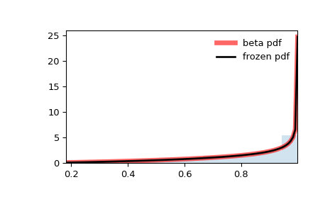
Display the probability density function (`pdf`):
```
>>> x = np.linspace(beta.ppf(0.01, a, b),
... beta.ppf(0.99, a, b), 100)
>>> ax.plot(x, beta.pdf(x, a, b),
... 'r-', lw=5, alpha=0.6, label='beta pdf')
```
Alternatively, the distribution object can be called (as a function) to fix the shape, location and scale parameters. This returns a “frozen” RV object holding the given parameters fixed.
Freeze the distribution and display the frozen `pdf`:
```
>>> rv = beta(a, b)
>>> ax.plot(x, rv.pdf(x), 'k-', lw=2, label='frozen pdf')
```
Check accuracy of `cdf` and `ppf`:
```
>>> vals = beta.ppf([0.001, 0.5, 0.999], a, b)
>>> np.allclose([0.001, 0.5, 0.999], beta.cdf(vals, a, b))
True
```
Generate random numbers:
```
>>> r = beta.rvs(a, b, size=1000)
```
And compare the histogram:
```
>>> ax.hist(r, density=True, bins='auto', histtype='stepfilled', alpha=0.2)
>>> ax.set_xlim([x[0], x[-1]])
>>> ax.legend(loc='best', frameon=False)
>>> plt.show()
```
Go Back
Open In Tab
[previous scipy.stats.argus](https://docs.scipy.org/doc/scipy/reference/generated/scipy.stats.argus.html "previous page")
[next scipy.stats.betaprime](https://docs.scipy.org/doc/scipy/reference/generated/scipy.stats.betaprime.html "next page")
On this page
- [`beta`](https://docs.scipy.org/doc/scipy/reference/generated/scipy.stats.beta.html#scipy.stats.beta)
© Copyright 2008, The SciPy community.
Created using [Sphinx](https://www.sphinx-doc.org/) 8.1.3.
Built with the [PyData Sphinx Theme](https://pydata-sphinx-theme.readthedocs.io/en/stable/index.html) 0.16.1. | ||||||||||||||||||
| Readable Markdown | scipy.stats.beta *\= \<scipy.stats.\_continuous\_distns.beta\_gen object\>*[\[source\]](https://github.com/scipy/scipy/blob/v1.17.0/scipy/stats/_continuous_distns.py#L708-L967)[\#](https://docs.scipy.org/doc/scipy/reference/generated/scipy.stats.beta.html#scipy.stats.beta "Link to this definition")
A beta continuous random variable.
As an instance of the [`rv_continuous`](https://docs.scipy.org/doc/scipy/reference/generated/scipy.stats.rv_continuous.html#scipy.stats.rv_continuous "scipy.stats.rv_continuous") class, [`beta`](https://docs.scipy.org/doc/scipy/reference/generated/scipy.stats.beta.html#scipy.stats.beta "scipy.stats.beta") object inherits from it a collection of generic methods (see below for the full list), and completes them with details specific for this particular distribution.
Methods
| | |
|---|---|
| **rvs(a, b, loc=0, scale=1, size=1, random\_state=None)** | Random variates. |
| **pdf(x, a, b, loc=0, scale=1)** | Probability density function. |
| **logpdf(x, a, b, loc=0, scale=1)** | Log of the probability density function. |
| **cdf(x, a, b, loc=0, scale=1)** | Cumulative distribution function. |
| **logcdf(x, a, b, loc=0, scale=1)** | Log of the cumulative distribution function. |
| **sf(x, a, b, loc=0, scale=1)** | Survival function (also defined as `1 - cdf`, but *sf* is sometimes more accurate). |
| **logsf(x, a, b, loc=0, scale=1)** | Log of the survival function. |
| **ppf(q, a, b, loc=0, scale=1)** | Percent point function (inverse of `cdf` — percentiles). |
| **isf(q, a, b, loc=0, scale=1)** | Inverse survival function (inverse of `sf`). |
| **moment(order, a, b, loc=0, scale=1)** | Non-central moment of the specified order. |
| **stats(a, b, loc=0, scale=1, moments=’mv’)** | Mean(‘m’), variance(‘v’), skew(‘s’), and/or kurtosis(‘k’). |
| **entropy(a, b, loc=0, scale=1)** | (Differential) entropy of the RV. |
| **fit(data)** | Parameter estimates for generic data. See [scipy.stats.rv\_continuous.fit](https://docs.scipy.org/doc/scipy/reference/generated/scipy.stats.rv_continuous.fit.html#scipy.stats.rv_continuous.fit) for detailed documentation of the keyword arguments. |
| **expect(func, args=(a, b), loc=0, scale=1, lb=None, ub=None, conditional=False, \*\*kwds)** | Expected value of a function (of one argument) with respect to the distribution. |
| **median(a, b, loc=0, scale=1)** | Median of the distribution. |
| **mean(a, b, loc=0, scale=1)** | Mean of the distribution. |
| **var(a, b, loc=0, scale=1)** | Variance of the distribution. |
| **std(a, b, loc=0, scale=1)** | Standard deviation of the distribution. |
| **interval(confidence, a, b, loc=0, scale=1)** | Confidence interval with equal areas around the median. |
Notes
The probability density function for [`beta`](https://docs.scipy.org/doc/scipy/reference/generated/scipy.stats.beta.html#scipy.stats.beta "scipy.stats.beta") is:
\\\[f(x, a, b) = \\frac{\\Gamma(a+b) x^{a-1} (1-x)^{b-1}} {\\Gamma(a) \\Gamma(b)}\\\]
for \\(0 \<= x \<= 1\\), \\(a \> 0\\), \\(b \> 0\\), where \\(\\Gamma\\) is the gamma function ([`scipy.special.gamma`](https://docs.scipy.org/doc/scipy/reference/generated/scipy.special.gamma.html#scipy.special.gamma "scipy.special.gamma")).
[`beta`](https://docs.scipy.org/doc/scipy/reference/generated/scipy.stats.beta.html#scipy.stats.beta "scipy.stats.beta") takes \\(a\\) and \\(b\\) as shape parameters.
This distribution uses routines from the Boost Math C++ library for the computation of the `pdf`, `cdf`, `ppf`, `sf` and `isf` methods. [\[1\]](https://docs.scipy.org/doc/scipy/reference/generated/scipy.stats.beta.html#r8b11f181b37f-1)
Maximum likelihood estimates of parameters are only available when the location and scale are fixed. When either of these parameters is free, `beta.fit` resorts to numerical optimization, but this problem is unbounded: the location and scale may be chosen to make the minimum and maximum elements of the data coincide with the endpoints of the support, and the shape parameters may be chosen to make the PDF at these points infinite. For best results, pass `floc` and `fscale` keyword arguments to fix the location and scale, or use [`scipy.stats.fit`](https://docs.scipy.org/doc/scipy/reference/generated/scipy.stats.fit.html#scipy.stats.fit "scipy.stats.fit") with `method='mse'`.
The probability density above is defined in the “standardized” form. To shift and/or scale the distribution use the `loc` and `scale` parameters. Specifically, `beta.pdf(x, a, b, loc, scale)` is identically equivalent to `beta.pdf(y, a, b) / scale` with `y = (x - loc) / scale`. Note that shifting the location of a distribution does not make it a “noncentral” distribution; noncentral generalizations of some distributions are available in separate classes.
References
Examples
```
>>> import numpy as np
>>> from scipy.stats import beta
>>> import matplotlib.pyplot as plt
>>> fig, ax = plt.subplots(1, 1)
```
Get the support:
```
>>> a, b = 2.31, 0.627
>>> lb, ub = beta.support(a, b)
```
Calculate the first four moments:
```
>>> mean, var, skew, kurt = beta.stats(a, b, moments='mvsk')
```
Display the probability density function (`pdf`):
```
>>> x = np.linspace(beta.ppf(0.01, a, b),
... beta.ppf(0.99, a, b), 100)
>>> ax.plot(x, beta.pdf(x, a, b),
... 'r-', lw=5, alpha=0.6, label='beta pdf')
```
Alternatively, the distribution object can be called (as a function) to fix the shape, location and scale parameters. This returns a “frozen” RV object holding the given parameters fixed.
Freeze the distribution and display the frozen `pdf`:
```
>>> rv = beta(a, b)
>>> ax.plot(x, rv.pdf(x), 'k-', lw=2, label='frozen pdf')
```
Check accuracy of `cdf` and `ppf`:
```
>>> vals = beta.ppf([0.001, 0.5, 0.999], a, b)
>>> np.allclose([0.001, 0.5, 0.999], beta.cdf(vals, a, b))
True
```
Generate random numbers:
```
>>> r = beta.rvs(a, b, size=1000)
```
And compare the histogram:
```
>>> ax.hist(r, density=True, bins='auto', histtype='stepfilled', alpha=0.2)
>>> ax.set_xlim([x[0], x[-1]])
>>> ax.legend(loc='best', frameon=False)
>>> plt.show()
```
 | ||||||||||||||||||
| ML Classification | |||||||||||||||||||
| ML Categories |
Raw JSON{
"/Science": 590,
"/Computers_and_Electronics": 506,
"/Computers_and_Electronics/Software": 459,
"/Science/Mathematics": 359,
"/Science/Mathematics/Statistics": 352,
"/Computers_and_Electronics/Software/Software_Utilities": 198
} | ||||||||||||||||||
| ML Page Types |
Raw JSON{
"/Document": 954,
"/Document/Manual": 945
} | ||||||||||||||||||
| ML Intent Types |
Raw JSON{
"Informational": 976
} | ||||||||||||||||||
| Content Metadata | |||||||||||||||||||
| Language | en | ||||||||||||||||||
| Author | null | ||||||||||||||||||
| Publish Time | not set | ||||||||||||||||||
| Original Publish Time | 2014-10-24 16:05:31 (11 years ago) | ||||||||||||||||||
| Republished | No | ||||||||||||||||||
| Word Count (Total) | 974 | ||||||||||||||||||
| Word Count (Content) | 843 | ||||||||||||||||||
| Links | |||||||||||||||||||
| External Links | 5 | ||||||||||||||||||
| Internal Links | 33 | ||||||||||||||||||
| Technical SEO | |||||||||||||||||||
| Meta Nofollow | No | ||||||||||||||||||
| Meta Noarchive | No | ||||||||||||||||||
| JS Rendered | No | ||||||||||||||||||
| Redirect Target | null | ||||||||||||||||||
| Performance | |||||||||||||||||||
| Download Time (ms) | 46 | ||||||||||||||||||
| TTFB (ms) | 46 | ||||||||||||||||||
| Download Size (bytes) | 8,203 | ||||||||||||||||||
| Shard | 63 (laksa) | ||||||||||||||||||
| Root Hash | 12122434965281355463 | ||||||||||||||||||
| Unparsed URL | org,scipy!docs,/doc/scipy/reference/generated/scipy.stats.beta.html s443 | ||||||||||||||||||