ℹ️ Skipped - page is already crawled
| Filter | Status | Condition | Details |
|---|---|---|---|
| HTTP status | PASS | download_http_code = 200 | HTTP 200 |
| Age cutoff | PASS | download_stamp > now() - 6 MONTH | 0.5 months ago |
| History drop | PASS | isNull(history_drop_reason) | No drop reason |
| Spam/ban | PASS | fh_dont_index != 1 AND ml_spam_score = 0 | ml_spam_score=0 |
| Canonical | PASS | meta_canonical IS NULL OR = '' OR = src_unparsed | Not set |
| Property | Value | |||||||||||||||
|---|---|---|---|---|---|---|---|---|---|---|---|---|---|---|---|---|
| URL | https://bookdown.org/pbaumgartner/bayesian-fun/05-beta-distribution.html | |||||||||||||||
| Last Crawled | 2026-04-07 00:17:11 (16 days ago) | |||||||||||||||
| First Indexed | 2023-09-14 20:55:16 (2 years ago) | |||||||||||||||
| HTTP Status Code | 200 | |||||||||||||||
| Content | ||||||||||||||||
| Meta Title | Bayesian Statistics the Fun Way - 5 The Beta Distribution | |||||||||||||||
| Meta Description | null | |||||||||||||||
| Meta Canonical | null | |||||||||||||||
| Boilerpipe Text | The chapter is concerned with two topics:
Beta Distribution
: You use the
beta distribution
to estimate the probability of an event for which you’ve already observed a number of trials and the number of successful outcomes. For example, you would use it to estimate the probability of flipping a heads when so far you have observed 100 tosses of a coin and 40 of those were heads.
Probability vs. Statistics
: Often in probability texts, we are given the probabilities for events explicitly. However, in real life, this is rarely the case. Instead, we are given data, which we use to come up with estimates for probabilities. This is where statistics comes in: it allows us to take data and make estimates about what probabilities we’re dealing with.
A Strange Scenario: Getting the Data
If you drop a quarter into a black box, it eject sometimes two quarter but sometimes it “eats” your quarter. So the question is: “What’s the probability of getting two quarters?”
Distinguishing Probability, Statistics, and Inference
In all of the examples so far, outside of the first chapter, we’ve known the probability of all the possible events, or at least how much we’d be willing to bet on them. In real life we are almost never sure what the exact probability of any event is; instead, we just have observations and data.
This is commonly considered the division between probability and statistics. In
probability
, we know exactly how probable all of our events are, and what we are concerned with is how likely certain observations are. For example, we might be told that there is 1/2 probability of getting heads in a fair coin toss and want to know the probability of getting exactly 7 heads in 20 coin tosses.
In
statistics
, we would look at this problem backward: assuming you observe 7 heads in 20 coin tosses, what is the probability of getting heads in a single coin toss? In a sense, statistics is probability in reverse. The task of figuring out probabilities given data is called
inference
, and it is the foundation of statistics.
Collecting Data
We want to estimate the probability that the mysterious box will deliver two quarters, and to do that, we first need to see how frequently you win after a few more tries. We’ve got 14 wins and 27 losses.
Without doing any further analysis, you might intuitively want to update your guess that P(two quarters) = 1/2 to P(two quarters) = 14/41. But what about your original guess—does your new data mean it’s impossible that 1/2 is the real probability?
Calculating the Probability of Probabilities
H
1
i
s
P
(
two coins
)
=
1
2
H
2
i
s
P
(
two coins
)
=
14
41
“How probable is what we observed if
H
1
were true versus if
H
2
were true?” We can easily calculate this using
Equation
4.6
of the binomial distribution from
Chapter 4
.
Listing 5.1: Calculating the Probability of Probabilities with dbinom()
#> [1] 0.01602537
Listing 5.2: Calculating the Probability of Probabilities with dbinom()
#> [1] 0.1304709
This shows us that, given the data (observing 14 cases of getting two coins out of 41 trials),
H
2
is almost 10 times more probable than
H
1
! However, it also shows that neither hypothesis is impossible and that there are, of course, many other hypotheses we could make based on our data.
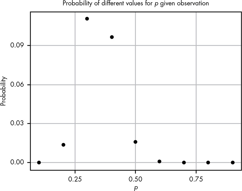
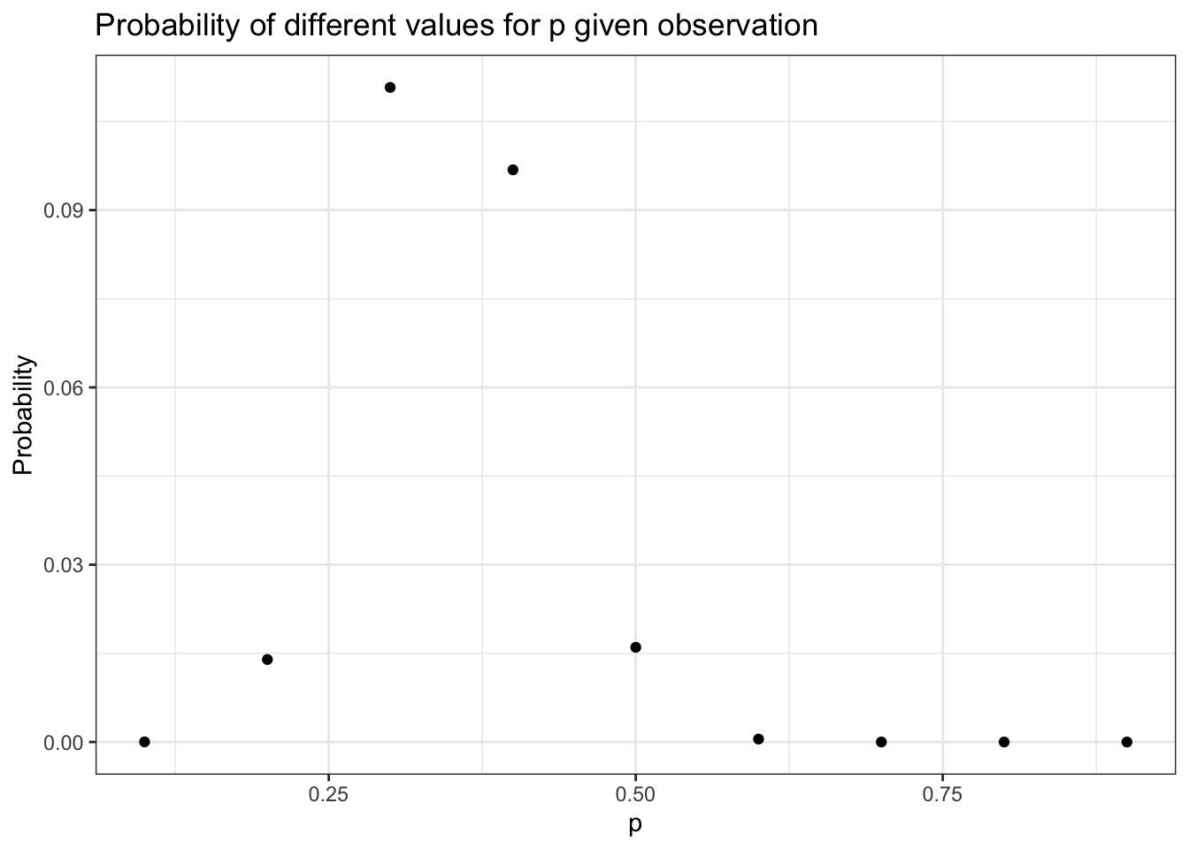
If we wanted to look for a pattern, we could pick every probability from 0.1 to 0.9, incrementing by 0.1; calculate the probability of the observed data in each distribution; and develop our hypothesis from that.
Figure 5.1: Visualization of different hypotheses about the rate of getting two quarters
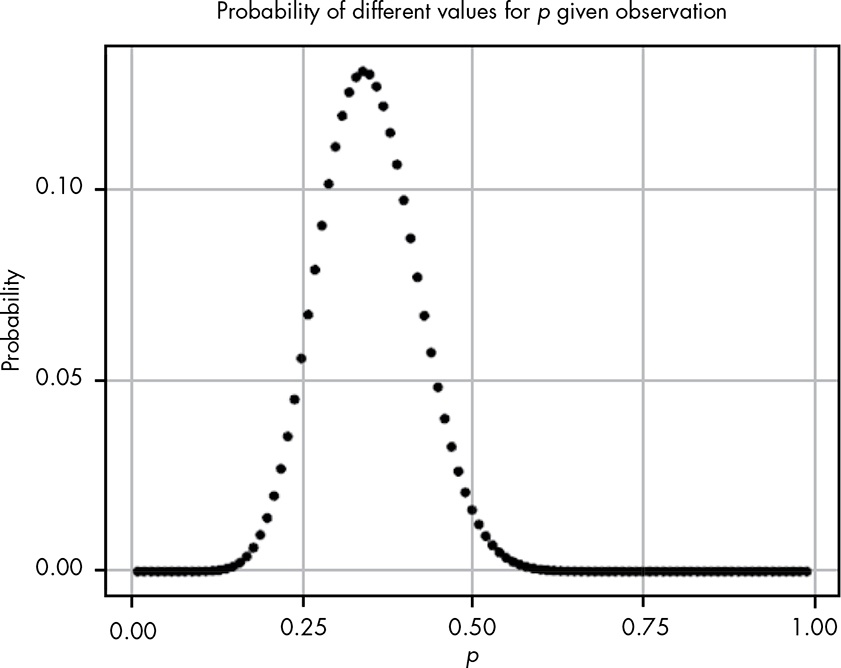
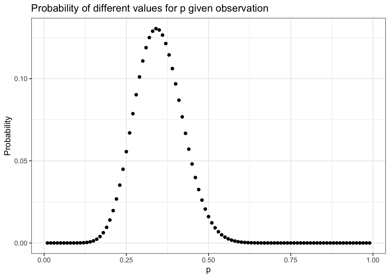
Even with all these hypotheses, there’s no way we could cover every possible eventuality because we’re not working with a finite number of hypotheses. So let’s try to get more information by testing more distributions. If we repeat the last experiment, testing each possibility at certain increments starting with 0.01 and ending with 0.99, incrementing by only 0.01 would give us the results in
Figure
5.2
.
Figure 5.2: We see a definite pattern emerging when we look at more hypotheses
This seems like valuable information; we can easily see where the probability is highest. Our goal, however, is to model our beliefs in all possible hypotheses (that is, the full probability distribution of our beliefs).
There are two problems:
There’s an infinite number of possible hypotheses, incrementing by smaller and smaller amounts doesn’t accurately represent the entire range of possibilities—we’re always missing an infinite amount. (In practice, this isn’t a huge problem.)
There are 11 dots above 0.1 right now, and we have an infinite number of points to add. This means that our probabilities don’t sum to 1!
Even though there are infinitely many possibilities here, we still need them all to sum to 1. This is where the beta distribution comes in.
Beta Distribution
Unlike the
binomial distribution
, which breaks up nicely into discrete values, the
beta distribution
represents a continuous range of values, which allows us to represent our infinite number of possible hypotheses.
We define the beta distribution with a probability density function (
PDF
), which is very similar to the probability mass function we use in the binomial distribution, but is defined for continuous values.
Theorem 5.1 (Formula for the PDF of the beta function)
(5.1)
B
e
t
a
(
p
;
α
,
β
)
=
p
α
−
1
×
(
1
−
p
)
β
−
1
b
e
t
a
(
α
,
β
)
Breaking Down the Probability Density Function
p
: Represents the probability of an event. This corresponds to our different hypotheses for the possible probabilities for our black box.
$\alpha$
: Represents how many times we observe an event we care about, such as getting two quarters from the box.
$\beta$
: Represents how many times the event we care about didn’t happen. For our example, this is the number of times that the black box ate the quarter.
$\alpha + \beta$
: The total number of trials. This is different than the binomial distribution, where we have
k
observations we’re interested in and a finite number of
n
total trials.
The top part of the
PDF
function should look pretty familiar because it’s almost the same as the binomial distribution’s
PMF
in
Equation
4.6
.
Differences between the PMF of the binomial distribution and the PDF of the beta distribution
:
In the PDF, rather than
p
k
×
(
1
−
p
)
n
−
k
, we have
p
α
−
1
×
(
1
−
p
)
β
−
1
where we subtract 1 from the exponent terms.
We also have another function in the denominator of our equation: the beta function (note the lowercase) for which the beta distribution is named. We subtract 1 from the exponent and use the beta function to normalize our values—this is the part that ensures our distribution sums to 1. The beta function is the integral from 0 to 1 of
p
α
−
1
×
(
1
−
p
)
β
−
1
. (A discussion of how subtracting 1 from the exponents and dividing by the beta functions normalizes our values is beyond the scope of this chapter.)
What we get in the end is a function that describes the probability of each possible hypothesis for our true belief in the probability of getting two heads from the box, given that we have observed
α
examples of one outcome and
β
examples of another. Remember that we arrived at the beta distribution by comparing how well different binomial distributions, each with its own probability
p
, described our data. In other words, the beta distribution represents how well all possible binomial distributions describe the data observed.
Applying the Probability Density Function to Our Problem
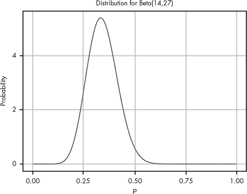
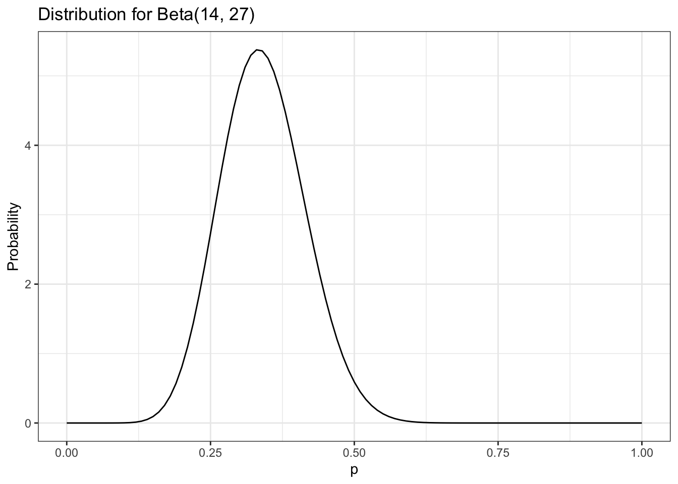
When we plug in our values for our black box data and visualize the beta distribution, shown in
Figure
5.3
, we see that it looks like a smooth version of the plot in
Figure
5.2
.
Figure 5.3: Visualizing the beta distribution for our data collected about the black box
While we can see the distribution of our beliefs by looking at a plot, we’d still like to be able to quantify exactly how strongly we believe that “the probability that the true rate at which the box returns two quarters is less than 0.5.”
Quantifying Continuous Distributions with Integration
The beta distribution is fundamentally different from the binomial distribution in that with the latter, we are looking at the distribution of
k
, the number of outcomes we care about, which is always something we can count. For the beta distribution, however, we are looking at the distribution of
p
, for which we have an infinite number of possible values.
We know that the fundamental rule of probability is that the sum of all our values must be 1, but each of our individual values is
infinitely
small, meaning the probability of any specific value is in practice 0.
Note
The zero probability of an event in a continuous distribution does not mean that this event never could happen. Zero probability only means that the events gets the probability measure of zero.
Our intuition from discrete probability is that if an outcome has zero probability, then the outcome is impossible. With continuous random variables (or more generally, an infinite number of possible outcomes) that intuition is flawed. (
StackExchange
)
For example, even if we divided a 1-pound bar of chocolate into infinitely many pieces, we can still add up the weight of the pieces in one half of the chocolate bar. Similarly, when talking about probability in continuous distributions, we can sum up ranges of values. But if every specific value is 0, then isn’t the sum just 0 as well?
This is where calculus comes in: in calculus, there’s a special way of summing up infinitely small values called the
integral.
If we want to know whether the probability that the box will return a coin is less than 0.5 (that is, the value is somewhere between 0 and 0.5), we can sum it up like this:
(5.2)
∫
0
0.5
p
14
−
1
×
(
1
−
p
)
27
−
1
b
e
t
a
(
14
,
27
)
R includes a function called
dbeta()
that is the PDF for the beta distribution. This function takes three arguments, corresponding to
p
,
α
, and
β
. We use this together with R’s
integrate()
function to perform this integration automatically. Here we calculate the probability that the chance of getting two coins from the box is less than or equal to 0.5, given the data:
Listing 5.3: Probability of getting two coins from the box is less than or equal to 0.5, given the data
#> 0.9807613 with absolute error < 5.9e-06
The “absolute error” message appears because computers can’t perfectly calculate integrals so there is always some error, though usually it is far too small for us to worry about. This result from R tells us that there is a 0.98 probability that, given our evidence, the true probability of getting two coins out of the black box is less than 0.5. This means it would not be good idea to put any more quarters in the box, since you very likely won’t break even.
Reverse-Engineering the Gacha Game
In real-life situations, we almost never know the true probabilities for events. That’s why the beta distribution is one of our most powerful tools for understanding our data.
In
Section 4.4
of
Chapter 4
, we knew the probability of the card we wanted to pull. In reality, the game developers are very unlikely to give players this information, for many reasons (such as not wanting players to calculate how unlikely they are to get the card they want).
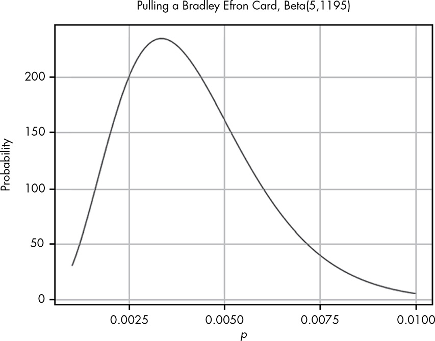
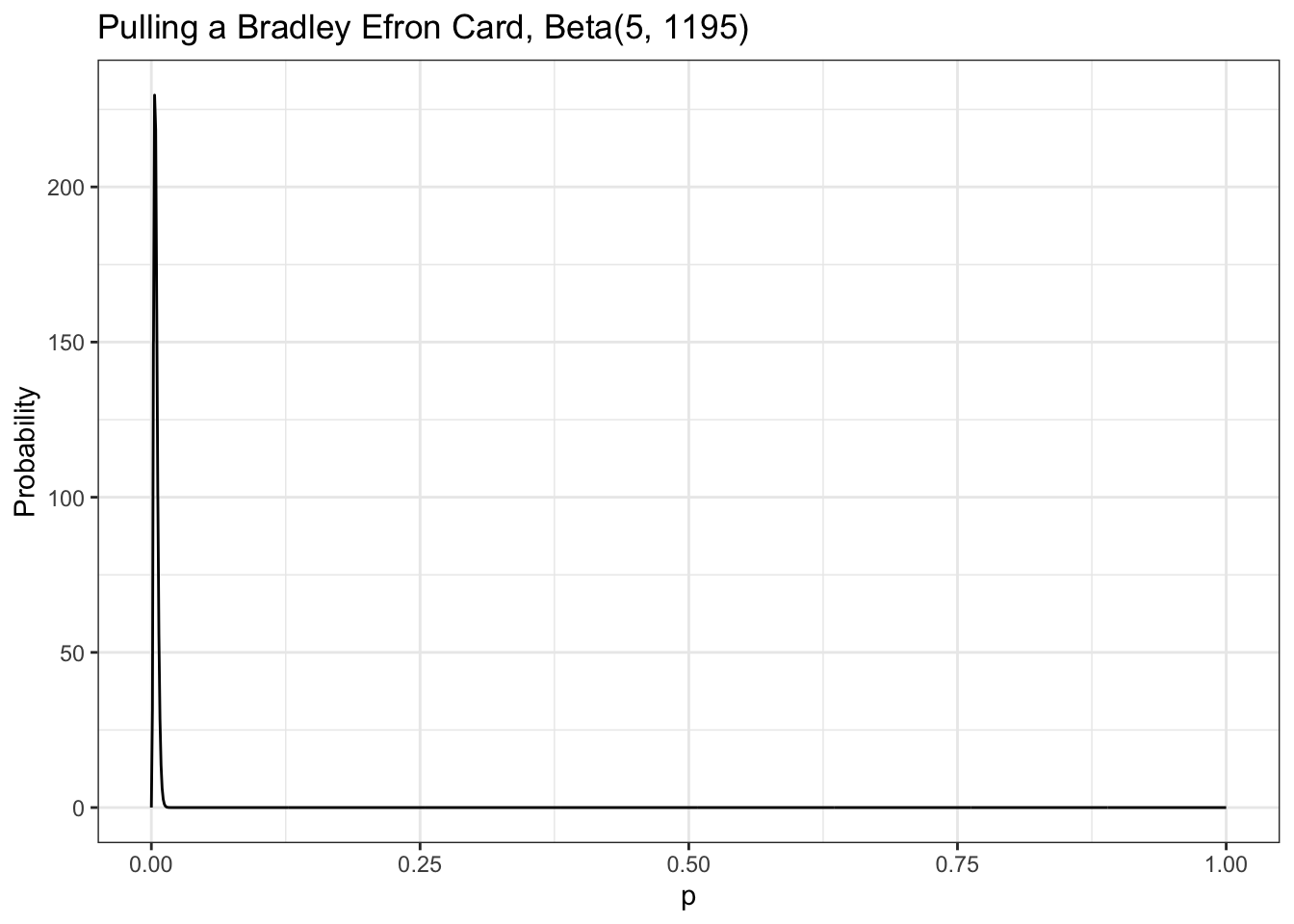
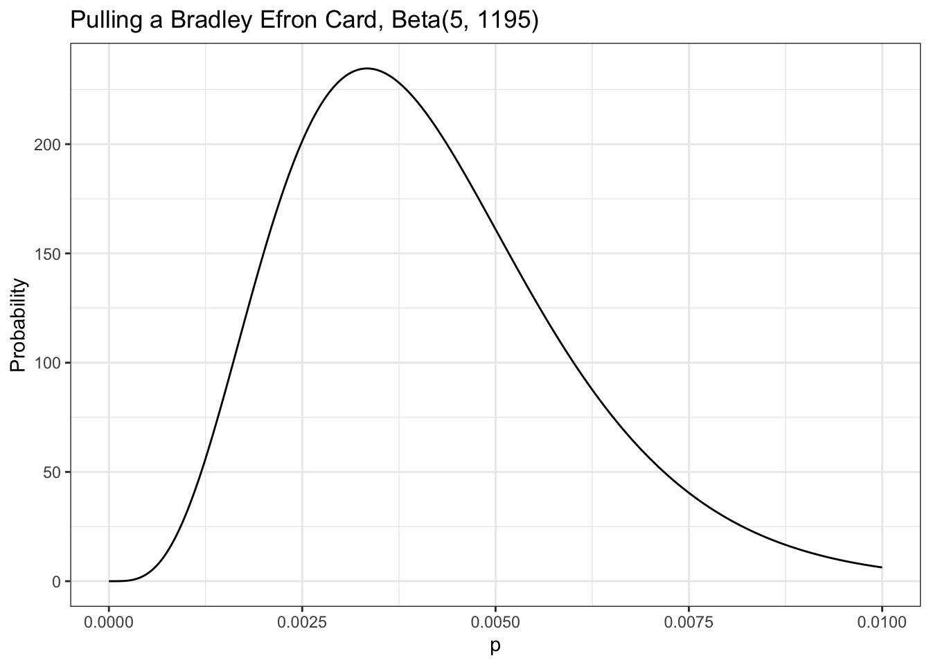
This time we don’t know the rates for the card, but we really want that card—and more than one if possible. We spend a ridiculous amount of money and find that from 1,200 cards pulled, we received only 5 cards we’re interested in. Our friend is thinking of spending money on the game but only wants to do it if there is a better than 0.7 probability that the chance of pulling the card is greater than 0.005.
Our data tells us that of 1,200 cards pulled, only 5 were cards we are interested in, so we can visualize this as Beta(5,1195), shown in
Figure
5.4
(remember that the total cards pulled is
α
+
β
).
Figure 5.4: The beta distribution for getting the card we are interested in, given our data
From our visualization we can see that nearly all the probability density is below 0.01. We need to know exactly how much is above 0.005, the value that our friend cares about. We can solve this by integrating over the beta distribution in R:
Listing 5.4: Probability that the rate of pulling a card we are interested is 0.005 or greater
#> 0.2850559 with absolute error < 1e-04
This tells us the probability that the rate of pulling a card we are interested is 0.005 or greater, given the evidence we have observed, is only 0.29. Our friend will pull for this card only if the probability is around 0.7 or greater, so based on the evidence from our data collection, our friend should not try his luck.
Wrapping Up
We learned about the beta distribution, which is closely related to the binomial distribution but behaves quite differently. The major difference between the beta distribution and the binomial distribution is that the beta distribution is a continuous probability distribution. Because there are an infinite number of values in the distribution, we cannot sum results the same way we do in a discrete probability distribution. Instead, we need to use calculus to sum ranges of values. Fortunately, we can use R instead of solving tricky integrals by hand.
We built up to the beta distribution by observing how well an increasing number of possible binomial distributions explained our data. The beta distribution allows us to represent how strongly we believe in all possible probabilities for the data we observed. This enables us to perform statistical inference on observed data by determining which probabilities we might assign to an event and how strongly we believe in each one: a
probability of probabilities
.
Exercises
Try answering the following questions to make sure you understand how we can use the Beta distribution to estimate probabilities. The solutions can be found at https://nostarch.com/learnbayes/.
Exercise 5-1
You want to use the
beta distribution
to determine whether or not a coin you have is a fair coin — meaning that the coin gives you heads and tails equally. You flip the coin 10 times and get 4 heads and 6 tails. Using the beta distribution, what is the probability that the coin will land on heads more than 60 percent of the time?
Listing 5.5: Probability that a coin will land on heads more than 60% given 4 heads in 10 tosses
#> 0.09935258 with absolute error < 1.1e-15
Exercise 5-2
You flip the coin 10 more times and now have 9 heads and 11 tails total. What is the probability that the coin is fair, using our definition of fair, give or take 5 percent?
Listing 5.6: Probability that a coin is fair within a 5% range given 9 heads in 20 tosses
#> 0.30988 with absolute error < 3.4e-15
Exercise 5-3
Data is the best way to become more confident in your assertions. You flip the coin 200 more times and end up with 109 heads and 111 tails. Now what is the probability that the coin is fair, give or take 5 percent?
Listing 5.7: Probability that a coin is fair within a 5% range given 109 heads in 220 tosses
#> 0.8589371 with absolute error < 9.5e-15
Experiments
Replicating Figure 5.1
To replicate
Figure
5.1
we need to pick every probability from 0.1 to 0.9, incrementing by 0.1; and then to calculate the probability of the observed data (14 cases of getting two coins out of 41 trials) in each distribution:
Listing 5.8: Replication of Figure 5.1: Visualization of different hypotheses about the rate of getting two quarters from the black box
tibble
::
tibble
(
x
=
seq
(
from
=
0.1
, to
=
0.9
, by
=
0.1
)
,
y
=
dbinom
(
14
,
41
,
x
)
)
|>
ggplot2
::
ggplot
(
ggplot2
::
aes
(
x
=
x
, y
=
y
)
)
+
ggplot2
::
geom_point
(
)
+
ggplot2
::
theme_bw
(
)
+
ggplot2
::
labs
(
title
=
"Probability of different values for p given observation"
,
x
=
"p"
,
y
=
"Probability"
)
Figure 5.5: Visualization of different hypotheses about the rate of getting two quarters from the black box
Replicating Figure 5.2
Repeating
Section 5.6.1
, we want to display each possibility at smaller increments starting with 0.01 and ending with 0.99, incrementing by only 0.01:
Listing 5.9: Replication of Figure 5.2: We see a definite pattern emerging when we look at more hypotheses
tibble
::
tibble
(
x
=
seq
(
from
=
0.01
, to
=
0.99
, by
=
0.01
)
,
y
=
dbinom
(
14
,
41
,
x
)
)
|>
ggplot2
::
ggplot
(
ggplot2
::
aes
(
x
=
x
, y
=
y
)
)
+
ggplot2
::
geom_point
(
)
+
ggplot2
::
theme_bw
(
)
+
ggplot2
::
labs
(
title
=
"Probability of different values for p given observation"
,
x
=
"p"
,
y
=
"Probability"
)
Figure 5.6: A definite pattern emerging when we look at more hypotheses
Replicating Figure 5.3
Our data: We’ve got 14 successes (two coins) with 41 trials.
Listing 5.10: Replication of Figure 5.3: Visualizing the beta distribution for our data collected about the black box
tibble
::
tibble
(
x
=
seq
(
from
=
0
, to
=
1
, by
=
0.01
)
,
y
=
dbeta
(
x
,
14
,
27
)
)
|>
ggplot2
::
ggplot
(
ggplot2
::
aes
(
x
=
x
, y
=
y
)
)
+
ggplot2
::
geom_line
(
)
+
ggplot2
::
theme_bw
(
)
+
ggplot2
::
labs
(
title
=
"Distribution for Beta(14, 27)"
,
x
=
"p"
,
y
=
"Probability"
)
Figure 5.7: Visualizing the beta distribution for our data collected about the black box
Replicating Figure 5.4
Our data tells us that of 1,200 cards pulled, there were only 5 cards we are interested in. Our friend is thinking of spending money on the game but only wants to do it if there is a better than 0.7 probability that the chance of pulling a Bradley Efron (the card we are interested) is greater than 0.005.
Listing 5.11: Replication of Figure 5.4: The beta distribution for getting the card we are interested in, given our data
tibble
::
tibble
(
x
=
seq
(
from
=
0
, to
=
1
, length
=
1000
)
,
y
=
dbeta
(
x
,
5
,
1195
)
)
|>
ggplot2
::
ggplot
(
ggplot2
::
aes
(
x
=
x
, y
=
y
)
)
+
ggplot2
::
geom_line
(
)
+
ggplot2
::
theme_bw
(
)
+
ggplot2
::
labs
(
title
=
"Pulling a Bradley Efron Card, Beta(5, 1195)"
,
x
=
"p"
,
y
=
"Probability"
)
Figure 5.8: The beta distribution form 0 to 1 for getting the card we are interested in, given our data
This was my first try. At first I thought that my
Listing
5.11
is wrong as
Figure
5.4
has a very different appearance. But then I noticed that my graphics displays value from 0 to 1 whereas
Figure
5.4
visualizes only values between 0 and 0.01!
In
Listing
5.12
I changed the visualization just showing values from 0 to 0.01.
Listing 5.12: Replication of Figure 5.4: The beta distribution for getting the card we are interested in, given our data
tibble
::
tibble
(
x
=
seq
(
from
=
0
, to
=
0.01
, length
=
1000
)
,
y
=
dbeta
(
x
,
5
,
1195
)
)
|>
ggplot2
::
ggplot
(
ggplot2
::
aes
(
x
=
x
, y
=
y
)
)
+
ggplot2
::
geom_line
(
)
+
ggplot2
::
theme_bw
(
)
+
ggplot2
::
labs
(
title
=
"Pulling a Bradley Efron Card, Beta(5, 1195)"
,
x
=
"p"
,
y
=
"Probability"
)
The beta distribution form 0 to 0.01 for getting the card we are interested in, given our data | |||||||||||||||
| Markdown | 1. [5 The Beta Distribution](https://bookdown.org/pbaumgartner/bayesian-fun/05-beta-distribution.html)
[Bayesian Statistics the Fun Way](https://bookdown.org/pbaumgartner/bayesian-fun/)
- [Preface](https://bookdown.org/pbaumgartner/bayesian-fun/)
- PART I: Introduction to Probability
- [Introduction](https://bookdown.org/pbaumgartner/bayesian-fun/00-intro.html)
- [1 Bayesian Thinking and Everyday Reasoning](https://bookdown.org/pbaumgartner/bayesian-fun/01-everyday-reasoning.html)
- [2 Measuring Uncertainty](https://bookdown.org/pbaumgartner/bayesian-fun/02-measuring-uncertainty.html)
- [3 Logic of Uncertainty](https://bookdown.org/pbaumgartner/bayesian-fun/03-logic-uncertainty.html)
- [4 Creating a Binomial Probability Distribution](https://bookdown.org/pbaumgartner/bayesian-fun/04-binomial-distribution.html)
- [5 The Beta Distribution](https://bookdown.org/pbaumgartner/bayesian-fun/05-beta-distribution.html)
- PART II: Bayesian Probability and Prior Probabilities
- [6 Conditional Probability](https://bookdown.org/pbaumgartner/bayesian-fun/06-conditional-probability.html)
- [7 Bayes’ Theorem With LEGO](https://bookdown.org/pbaumgartner/bayesian-fun/07-bayes-lego.html)
- [8 The Prior, Likelihood, and Posterior of Bayes’ Theorem](https://bookdown.org/pbaumgartner/bayesian-fun/08-prior-likelihood-posterior.html)
- [9 Bayesian Priors and Working with Probability Distributions](https://bookdown.org/pbaumgartner/bayesian-fun/09-probability-distributions.html)
- PART III: Parameter Estimation
- [10 Introduction to Averaging and Parameter Estimation](https://bookdown.org/pbaumgartner/bayesian-fun/10-parameter-estimation.html)
- [11 Measuring the Spread of our Data](https://bookdown.org/pbaumgartner/bayesian-fun/11-data-spread.html)
- [12 The Normal Distribution](https://bookdown.org/pbaumgartner/bayesian-fun/12-normal-distribution.html)
- [13 Tools of Parameter Estimation: The PDF, CDF, and Quantile Function](https://bookdown.org/pbaumgartner/bayesian-fun/13-pdf-cdf-quantile.html)
- [14 Parameter Estimation with Prior Probabilities](https://bookdown.org/pbaumgartner/bayesian-fun/14-prior-probabilities.html)
- PART IV: Hypothesis Testing: The Heart of Statistics
- [15 From Parameter Estimation to Hypothesis Testing: Building a Bayesian A/B Test](https://bookdown.org/pbaumgartner/bayesian-fun/15-bayesian-a-b-test.html)
- [16 Introduction to the Bayes Factor and Posterior Odds: The Competition of Ideas](https://bookdown.org/pbaumgartner/bayesian-fun/16-bayes-factor-posterior-odds.html)
- [17 Bayesian Reasoning in the Twilight Zone](https://bookdown.org/pbaumgartner/bayesian-fun/17-bayesian-reasoning.html)
- [18 When Data Doesn’t Convince](https://bookdown.org/pbaumgartner/bayesian-fun/18-data-convince.html)
- [19 From Hypothesis Testing to Parameter Estimation](https://bookdown.org/pbaumgartner/bayesian-fun/19-hypothesis-testing-parameter-estimation.html)
- [References](https://bookdown.org/pbaumgartner/bayesian-fun/95-references.html)
- [Appendices]()
- [A A Quick Introduction to R](https://bookdown.org/pbaumgartner/bayesian-fun/96-intro-to-r.html)
- [B Enough Calculus to Get By](https://bookdown.org/pbaumgartner/bayesian-fun/97-calculus.html)
## Table of contents
- [5\.1 A Strange Scenario: Getting the Data](https://bookdown.org/pbaumgartner/bayesian-fun/05-beta-distribution.html#a-strange-scenario-getting-the-data)
- [5\.1.1 Distinguishing Probability, Statistics, and Inference](https://bookdown.org/pbaumgartner/bayesian-fun/05-beta-distribution.html#distinguishing-probability-statistics-and-inference)
- [5\.1.2 Collecting Data](https://bookdown.org/pbaumgartner/bayesian-fun/05-beta-distribution.html#collecting-data)
- [5\.1.3 Calculating the Probability of Probabilities](https://bookdown.org/pbaumgartner/bayesian-fun/05-beta-distribution.html#calculating-the-probability-of-probabilities)
- [5\.2 Beta Distribution](https://bookdown.org/pbaumgartner/bayesian-fun/05-beta-distribution.html#sec-beta-distribution)
- [5\.2.1 Breaking Down the Probability Density Function](https://bookdown.org/pbaumgartner/bayesian-fun/05-beta-distribution.html#breaking-down-the-probability-density-function)
- [5\.2.2 Applying the Probability Density Function to Our Problem](https://bookdown.org/pbaumgartner/bayesian-fun/05-beta-distribution.html#applying-the-probability-density-function-to-our-problem)
- [5\.2.3 Quantifying Continuous Distributions with Integration](https://bookdown.org/pbaumgartner/bayesian-fun/05-beta-distribution.html#quantifying-continuous-distributions-with-integration)
- [5\.3 Reverse-Engineering the Gacha Game](https://bookdown.org/pbaumgartner/bayesian-fun/05-beta-distribution.html#reverse-engineering-the-gacha-game)
- [5\.4 Wrapping Up](https://bookdown.org/pbaumgartner/bayesian-fun/05-beta-distribution.html#wrapping-up)
- [5\.5 Exercises](https://bookdown.org/pbaumgartner/bayesian-fun/05-beta-distribution.html#exercises)
- [5\.5.1 Exercise 5-1](https://bookdown.org/pbaumgartner/bayesian-fun/05-beta-distribution.html#exercise-5-1)
- [5\.5.2 Exercise 5-2](https://bookdown.org/pbaumgartner/bayesian-fun/05-beta-distribution.html#exercise-5-2)
- [5\.5.3 Exercise 5-3](https://bookdown.org/pbaumgartner/bayesian-fun/05-beta-distribution.html#exercise-5-3)
- [5\.6 Experiments](https://bookdown.org/pbaumgartner/bayesian-fun/05-beta-distribution.html#experiments)
- [5\.6.1 Replicating Figure 5.1](https://bookdown.org/pbaumgartner/bayesian-fun/05-beta-distribution.html#sec-experiment-5-1)
- [5\.6.2 Replicating Figure 5.2](https://bookdown.org/pbaumgartner/bayesian-fun/05-beta-distribution.html#replicating-figure-5.2)
- [5\.6.3 Replicating Figure 5.3](https://bookdown.org/pbaumgartner/bayesian-fun/05-beta-distribution.html#replicating-figure-5.3)
- [5\.6.4 Replicating Figure 5.4](https://bookdown.org/pbaumgartner/bayesian-fun/05-beta-distribution.html#replicating-figure-5.4)
# 5 The Beta Distribution
Code
The chapter is concerned with two topics:
- **Beta Distribution**: You use the [beta distribution]("It is a family of continuous probability distributions defined on the interval [0, 1] in terms of two positive parameters, denoted by alpha (α) and beta (β) that control the shape of the distribution. (Wikipedia) The Beta distribution is representing a probability distribution of probabilities (stats.stackexchange) You use the beta distribution to estimate the probability of an event for which you’ve already observed a number of trials and the number of successful outcomes. For example, you would use it to estimate the probability of flipping a heads when so far you have observed 100 tosses of a coin and 40 of those were heads. (BF, Chap.5)") to estimate the probability of an event for which you’ve already observed a number of trials and the number of successful outcomes. For example, you would use it to estimate the probability of flipping a heads when so far you have observed 100 tosses of a coin and 40 of those were heads.
- **Probability vs. Statistics**: Often in probability texts, we are given the probabilities for events explicitly. However, in real life, this is rarely the case. Instead, we are given data, which we use to come up with estimates for probabilities. This is where statistics comes in: it allows us to take data and make estimates about what probabilities we’re dealing with.
## 5\.1 A Strange Scenario: Getting the Data
If you drop a quarter into a black box, it eject sometimes two quarter but sometimes it “eats” your quarter. So the question is: “What’s the probability of getting two quarters?”
### 5\.1.1 Distinguishing Probability, Statistics, and Inference
In all of the examples so far, outside of the first chapter, we’ve known the probability of all the possible events, or at least how much we’d be willing to bet on them. In real life we are almost never sure what the exact probability of any event is; instead, we just have observations and data.
This is commonly considered the division between probability and statistics. In [probability]("Probability is a mathematical tool used to study randomness. It deals with the chance of an event occurring. (OpenStax: Statistics) In the discrete case, to calculate the probability that a random variable takes on any value within a range, we sum the individual probabilities corresponding to each of the values. We use Pr to explicitly state that the result is a probability from a discrete probability distribution, whereas p(value) is a probability density from a continuous probability distribution. (Bayesian Statistics, Chap.3)"), we know exactly how probable all of our events are, and what we are concerned with is how likely certain observations are. For example, we might be told that there is 1/2 probability of getting heads in a fair coin toss and want to know the probability of getting exactly 7 heads in 20 coin tosses.
In [statistics]("Statistics is the discipline that concerns the collection, organization, analysis, interpretation, and presentation of data. Two main statistical methods are used in data analysis: descriptive statistics, which summarize data from a sample using, and inferential statistics, which draw conclusions from data."), we would look at this problem backward: assuming you observe 7 heads in 20 coin tosses, what is the probability of getting heads in a single coin toss? In a sense, statistics is probability in reverse. The task of figuring out probabilities given data is called [inference]("Statistical inference is the process of using data analysis to infer properties of an underlying distribution of probability. It makes propositions about a population, using data drawn from the population with some form of sampling. Given a hypothesis about a population, for which we wish to draw inferences, statistical inference consists of (first) selecting a statistical model of the process that generates the data and (second) deducing propositions from the model. Inferential statistics can be contrasted with descriptive statistics. (Wikipedia)"), and it is the foundation of statistics.
### 5\.1.2 Collecting Data
We want to estimate the probability that the mysterious box will deliver two quarters, and to do that, we first need to see how frequently you win after a few more tries. We’ve got 14 wins and 27 losses.
Without doing any further analysis, you might intuitively want to update your guess that P(two quarters) = 1/2 to P(two quarters) = 14/41. But what about your original guess—does your new data mean it’s impossible that 1/2 is the real probability?
### 5\.1.3 Calculating the Probability of Probabilities
H 1 i s P ( two coins ) \= 1 2 H 2 i s P ( two coins ) \= 14 41 “How probable is what we observed if H 1 were true versus if H 2 were true?” We can easily calculate this using [Equation 4\.6](https://bookdown.org/pbaumgartner/bayesian-fun/04-binomial-distribution.html#eq-pmf) of the binomial distribution from [Chapter 4](https://bookdown.org/pbaumgartner/bayesian-fun/04-binomial-distribution.html).
Listing 5.1: Calculating the Probability of Probabilities with dbinom()
```
(H1 <- dbinom(14, 41, 1/2))
```
```
#> [1] 0.01602537
```
Listing 5.2: Calculating the Probability of Probabilities with dbinom()
```
(H2 <- dbinom(14, 41, 14/41))
```
```
#> [1] 0.1304709
```
This shows us that, given the data (observing 14 cases of getting two coins out of 41 trials), H 2 is almost 10 times more probable than H 1! However, it also shows that neither hypothesis is impossible and that there are, of course, many other hypotheses we could make based on our data.
If we wanted to look for a pattern, we could pick every probability from 0.1 to 0.9, incrementing by 0.1; calculate the probability of the observed data in each distribution; and develop our hypothesis from that.
Figure 5.1: Visualization of different hypotheses about the rate of getting two quarters
Even with all these hypotheses, there’s no way we could cover every possible eventuality because we’re not working with a finite number of hypotheses. So let’s try to get more information by testing more distributions. If we repeat the last experiment, testing each possibility at certain increments starting with 0.01 and ending with 0.99, incrementing by only 0.01 would give us the results in [Figure 5\.2](https://bookdown.org/pbaumgartner/bayesian-fun/05-beta-distribution.html#fig-05-02).
Figure 5.2: We see a definite pattern emerging when we look at more hypotheses
This seems like valuable information; we can easily see where the probability is highest. Our goal, however, is to model our beliefs in all possible hypotheses (that is, the full probability distribution of our beliefs).
There are two problems:
1. There’s an infinite number of possible hypotheses, incrementing by smaller and smaller amounts doesn’t accurately represent the entire range of possibilities—we’re always missing an infinite amount. (In practice, this isn’t a huge problem.)
2. There are 11 dots above 0.1 right now, and we have an infinite number of points to add. This means that our probabilities don’t sum to 1\!
Even though there are infinitely many possibilities here, we still need them all to sum to 1. This is where the beta distribution comes in.
## 5\.2 Beta Distribution
Unlike the [binomial distribution]("It is used to calculate the probability of a certain number of successful outcomes, given a number of trials and the probability of the successful outcome. The “bi” in the term binomial refers to the two possible outcomes: an event happening and an event not happening. (BF, Chap.4)"), which breaks up nicely into discrete values, the [beta distribution]("It is a family of continuous probability distributions defined on the interval [0, 1] in terms of two positive parameters, denoted by alpha (α) and beta (β) that control the shape of the distribution. (Wikipedia) The Beta distribution is representing a probability distribution of probabilities (stats.stackexchange) You use the beta distribution to estimate the probability of an event for which you’ve already observed a number of trials and the number of successful outcomes. For example, you would use it to estimate the probability of flipping a heads when so far you have observed 100 tosses of a coin and 40 of those were heads. (BF, Chap.5)") represents a continuous range of values, which allows us to represent our infinite number of possible hypotheses.
We define the beta distribution with a probability density function ([PDF]("A probability densitiy function (PDF) describes a probability distribution for a random, continuous variable. Use a probability density function to find the chances that the value of a random variable will occur within a range of values that you specify. More specifically, a PDF is a function where its integral for an interval provides the probability of a value occurring in that interval. (Statistics By Jim)")), which is very similar to the probability mass function we use in the binomial distribution, but is defined for continuous values.
**Theorem 5.1 (Formula for the PDF of the beta function)** (5.1) B e t a ( p ; α , β ) \= p α − 1 × ( 1 − p ) β − 1 b e t a ( α , β )
### 5\.2.1 Breaking Down the Probability Density Function
`p`: Represents the probability of an event. This corresponds to our different hypotheses for the possible probabilities for our black box.
`$\alpha$`: Represents how many times we observe an event we care about, such as getting two quarters from the box.
`$\beta$`: Represents how many times the event we care about didn’t happen. For our example, this is the number of times that the black box ate the quarter.
`$\alpha + \beta$`: The total number of trials. This is different than the binomial distribution, where we have `k` observations we’re interested in and a finite number of `n` total trials.
The top part of the [PDF]("A probability densitiy function (PDF) describes a probability distribution for a random, continuous variable. Use a probability density function to find the chances that the value of a random variable will occur within a range of values that you specify. More specifically, a PDF is a function where its integral for an interval provides the probability of a value occurring in that interval. (Statistics By Jim)") function should look pretty familiar because it’s almost the same as the binomial distribution’s [PMF]("A probability mass function (PMF) is a mathematical function that calculates the probability a discrete random variable will be a specific value. PMFs also describe the probability distribution for the full range of values for a discrete variable. Probability mass functions find the LIKELIHOOD of a particular outcome. Using a PMF to calculate the likelihoods for all possible values of the discrete variable produces its PROBABILITY DISTRIBUTION.(Statistics By Jim)") in [Equation 4\.6](https://bookdown.org/pbaumgartner/bayesian-fun/04-binomial-distribution.html#eq-pmf).
**Differences between the PMF of the binomial distribution and the PDF of the beta distribution**:
- In the PDF, rather than
p
k
×
(
1
−
p
)
n
−
k
, we have
p
α
−
1
×
(
1
−
p
)
β
−
1
where we subtract 1 from the exponent terms.
- We also have another function in the denominator of our equation: the beta function (note the lowercase) for which the beta distribution is named. We subtract 1 from the exponent and use the beta function to normalize our values—this is the part that ensures our distribution sums to 1. The beta function is the integral from 0 to 1 of
p
α
−
1
×
(
1
−
p
)
β
−
1
. (A discussion of how subtracting 1 from the exponents and dividing by the beta functions normalizes our values is beyond the scope of this chapter.)
What we get in the end is a function that describes the probability of each possible hypothesis for our true belief in the probability of getting two heads from the box, given that we have observed α examples of one outcome and β examples of another. Remember that we arrived at the beta distribution by comparing how well different binomial distributions, each with its own probability p, described our data. In other words, the beta distribution represents how well all possible binomial distributions describe the data observed.
### 5\.2.2 Applying the Probability Density Function to Our Problem
When we plug in our values for our black box data and visualize the beta distribution, shown in [Figure 5\.3](https://bookdown.org/pbaumgartner/bayesian-fun/05-beta-distribution.html#fig-05-03), we see that it looks like a smooth version of the plot in [Figure 5\.2](https://bookdown.org/pbaumgartner/bayesian-fun/05-beta-distribution.html#fig-05-02).
Figure 5.3: Visualizing the beta distribution for our data collected about the black box
While we can see the distribution of our beliefs by looking at a plot, we’d still like to be able to quantify exactly how strongly we believe that “the probability that the true rate at which the box returns two quarters is less than 0.5.”
### 5\.2.3 Quantifying Continuous Distributions with Integration
The beta distribution is fundamentally different from the binomial distribution in that with the latter, we are looking at the distribution of k, the number of outcomes we care about, which is always something we can count. For the beta distribution, however, we are looking at the distribution of p, for which we have an infinite number of possible values.
We know that the fundamental rule of probability is that the sum of all our values must be 1, but each of our individual values is *infinitely* small, meaning the probability of any specific value is in practice 0.
Note
The zero probability of an event in a continuous distribution does not mean that this event never could happen. Zero probability only means that the events gets the probability measure of zero.
Our intuition from discrete probability is that if an outcome has zero probability, then the outcome is impossible. With continuous random variables (or more generally, an infinite number of possible outcomes) that intuition is flawed. ([StackExchange](https://stats.stackexchange.com/a/273398/207389))
For example, even if we divided a 1-pound bar of chocolate into infinitely many pieces, we can still add up the weight of the pieces in one half of the chocolate bar. Similarly, when talking about probability in continuous distributions, we can sum up ranges of values. But if every specific value is 0, then isn’t the sum just 0 as well?
This is where calculus comes in: in calculus, there’s a special way of summing up infinitely small values called the *integral.*
If we want to know whether the probability that the box will return a coin is less than 0.5 (that is, the value is somewhere between 0 and 0.5), we can sum it up like this:
(5.2) ∫ 0 0\.5 p 14 − 1 × ( 1 − p ) 27 − 1 b e t a ( 14 , 27 )
R includes a function called `dbeta()` that is the PDF for the beta distribution. This function takes three arguments, corresponding to p, α, and β. We use this together with R’s `integrate()` function to perform this integration automatically. Here we calculate the probability that the chance of getting two coins from the box is less than or equal to 0.5, given the data:
Listing 5.3: Probability of getting two coins from the box is less than or equal to 0.5, given the data
```
integrate(function(p) dbeta(p,14,27),0,0.5)
```
```
#> 0.9807613 with absolute error < 5.9e-06
```
The “absolute error” message appears because computers can’t perfectly calculate integrals so there is always some error, though usually it is far too small for us to worry about. This result from R tells us that there is a 0.98 probability that, given our evidence, the true probability of getting two coins out of the black box is less than 0.5. This means it would not be good idea to put any more quarters in the box, since you very likely won’t break even.
## 5\.3 Reverse-Engineering the Gacha Game
In real-life situations, we almost never know the true probabilities for events. That’s why the beta distribution is one of our most powerful tools for understanding our data.
In [Section 4.4](https://bookdown.org/pbaumgartner/bayesian-fun/04-binomial-distribution.html#sec-gacha-games) of [Chapter 4](https://bookdown.org/pbaumgartner/bayesian-fun/04-binomial-distribution.html) , we knew the probability of the card we wanted to pull. In reality, the game developers are very unlikely to give players this information, for many reasons (such as not wanting players to calculate how unlikely they are to get the card they want).
This time we don’t know the rates for the card, but we really want that card—and more than one if possible. We spend a ridiculous amount of money and find that from 1,200 cards pulled, we received only 5 cards we’re interested in. Our friend is thinking of spending money on the game but only wants to do it if there is a better than 0.7 probability that the chance of pulling the card is greater than 0.005.
Our data tells us that of 1,200 cards pulled, only 5 were cards we are interested in, so we can visualize this as Beta(5,1195), shown in [Figure 5\.4](https://bookdown.org/pbaumgartner/bayesian-fun/05-beta-distribution.html#fig-05-04) (remember that the total cards pulled is α \+ β).
Figure 5.4: The beta distribution for getting the card we are interested in, given our data
From our visualization we can see that nearly all the probability density is below 0.01. We need to know exactly how much is above 0.005, the value that our friend cares about. We can solve this by integrating over the beta distribution in R:
Listing 5.4: Probability that the rate of pulling a card we are interested is 0.005 or greater
```
integrate(function(x) dbeta(x,5,1195),0.005,1)
```
```
#> 0.2850559 with absolute error < 1e-04
```
This tells us the probability that the rate of pulling a card we are interested is 0.005 or greater, given the evidence we have observed, is only 0.29. Our friend will pull for this card only if the probability is around 0.7 or greater, so based on the evidence from our data collection, our friend should not try his luck.
## 5\.4 Wrapping Up
We learned about the beta distribution, which is closely related to the binomial distribution but behaves quite differently. The major difference between the beta distribution and the binomial distribution is that the beta distribution is a continuous probability distribution. Because there are an infinite number of values in the distribution, we cannot sum results the same way we do in a discrete probability distribution. Instead, we need to use calculus to sum ranges of values. Fortunately, we can use R instead of solving tricky integrals by hand.
We built up to the beta distribution by observing how well an increasing number of possible binomial distributions explained our data. The beta distribution allows us to represent how strongly we believe in all possible probabilities for the data we observed. This enables us to perform statistical inference on observed data by determining which probabilities we might assign to an event and how strongly we believe in each one: a *probability of probabilities*.
## 5\.5 Exercises
Try answering the following questions to make sure you understand how we can use the Beta distribution to estimate probabilities. The solutions can be found at https://nostarch.com/learnbayes/.
### 5\.5.1 Exercise 5-1
You want to use the [beta distribution]("It is a family of continuous probability distributions defined on the interval [0, 1] in terms of two positive parameters, denoted by alpha (α) and beta (β) that control the shape of the distribution. (Wikipedia) The Beta distribution is representing a probability distribution of probabilities (stats.stackexchange) You use the beta distribution to estimate the probability of an event for which you’ve already observed a number of trials and the number of successful outcomes. For example, you would use it to estimate the probability of flipping a heads when so far you have observed 100 tosses of a coin and 40 of those were heads. (BF, Chap.5)") to determine whether or not a coin you have is a fair coin — meaning that the coin gives you heads and tails equally. You flip the coin 10 times and get 4 heads and 6 tails. Using the beta distribution, what is the probability that the coin will land on heads more than 60 percent of the time?
Listing 5.5: Probability that a coin will land on heads more than 60% given 4 heads in 10 tosses
```
integrate(function(p) dbeta(p, 4, 6), 0.6, 1)
```
```
#> 0.09935258 with absolute error < 1.1e-15
```
### 5\.5.2 Exercise 5-2
You flip the coin 10 more times and now have 9 heads and 11 tails total. What is the probability that the coin is fair, using our definition of fair, give or take 5 percent?
Listing 5.6: Probability that a coin is fair within a 5% range given 9 heads in 20 tosses
```
integrate(function(p) dbeta(p, 9, 11), 0.45, 0.55)
```
```
#> 0.30988 with absolute error < 3.4e-15
```
### 5\.5.3 Exercise 5-3
Data is the best way to become more confident in your assertions. You flip the coin 200 more times and end up with 109 heads and 111 tails. Now what is the probability that the coin is fair, give or take 5 percent?
Listing 5.7: Probability that a coin is fair within a 5% range given 109 heads in 220 tosses
```
integrate(function(p) dbeta(p, 109, 111), 0.45, 0.55)
```
```
#> 0.8589371 with absolute error < 9.5e-15
```
## 5\.6 Experiments
### 5\.6.1 Replicating Figure 5.1
To replicate [Figure 5\.1](https://bookdown.org/pbaumgartner/bayesian-fun/05-beta-distribution.html#fig-05-01) we need to pick every probability from 0.1 to 0.9, incrementing by 0.1; and then to calculate the probability of the observed data (14 cases of getting two coins out of 41 trials) in each distribution:
Listing 5.8: Replication of Figure 5.1: Visualization of different hypotheses about the rate of getting two quarters from the black box
```
```
Figure 5.5: Visualization of different hypotheses about the rate of getting two quarters from the black box
### 5\.6.2 Replicating Figure 5.2
Repeating [Section 5.6.1](https://bookdown.org/pbaumgartner/bayesian-fun/05-beta-distribution.html#sec-experiment-5-1), we want to display each possibility at smaller increments starting with 0.01 and ending with 0.99, incrementing by only 0.01:
Listing 5.9: Replication of Figure 5.2: We see a definite pattern emerging when we look at more hypotheses
```
```
Figure 5.6: A definite pattern emerging when we look at more hypotheses
### 5\.6.3 Replicating Figure 5.3
Our data: We’ve got 14 successes (two coins) with 41 trials.
Listing 5.10: Replication of Figure 5.3: Visualizing the beta distribution for our data collected about the black box
```
```
Figure 5.7: Visualizing the beta distribution for our data collected about the black box
### 5\.6.4 Replicating Figure 5.4
Our data tells us that of 1,200 cards pulled, there were only 5 cards we are interested in. Our friend is thinking of spending money on the game but only wants to do it if there is a better than 0.7 probability that the chance of pulling a Bradley Efron (the card we are interested) is greater than 0.005.
Listing 5.11: Replication of Figure 5.4: The beta distribution for getting the card we are interested in, given our data
```
```
Figure 5.8: The beta distribution form 0 to 1 for getting the card we are interested in, given our data
This was my first try. At first I thought that my [Listing 5\.11](https://bookdown.org/pbaumgartner/bayesian-fun/05-beta-distribution.html#lst-fig-repl-5-4a) is wrong as [Figure 5\.4](https://bookdown.org/pbaumgartner/bayesian-fun/05-beta-distribution.html#fig-05-04) has a very different appearance. But then I noticed that my graphics displays value from 0 to 1 whereas [Figure 5\.4](https://bookdown.org/pbaumgartner/bayesian-fun/05-beta-distribution.html#fig-05-04) visualizes only values between 0 and 0.01\!
In [Listing 5\.12](https://bookdown.org/pbaumgartner/bayesian-fun/05-beta-distribution.html#lst-fig-repl-5-4b) I changed the visualization just showing values from 0 to 0.01.
Listing 5.12: Replication of Figure 5.4: The beta distribution for getting the card we are interested in, given our data
```
```
The beta distribution form 0 to 0.01 for getting the card we are interested in, given our data
[4 Creating a Binomial Probability Distribution](https://bookdown.org/pbaumgartner/bayesian-fun/04-binomial-distribution.html)
[6 Conditional Probability](https://bookdown.org/pbaumgartner/bayesian-fun/06-conditional-probability.html)
##### Source Code
```
``` | |||||||||||||||
| Readable Markdown | The chapter is concerned with two topics:
- **Beta Distribution**: You use the [beta distribution]("It is a family of continuous probability distributions defined on the interval [0, 1] in terms of two positive parameters, denoted by alpha (α) and beta (β) that control the shape of the distribution. (Wikipedia) The Beta distribution is representing a probability distribution of probabilities (stats.stackexchange) You use the beta distribution to estimate the probability of an event for which you’ve already observed a number of trials and the number of successful outcomes. For example, you would use it to estimate the probability of flipping a heads when so far you have observed 100 tosses of a coin and 40 of those were heads. (BF, Chap.5)") to estimate the probability of an event for which you’ve already observed a number of trials and the number of successful outcomes. For example, you would use it to estimate the probability of flipping a heads when so far you have observed 100 tosses of a coin and 40 of those were heads.
- **Probability vs. Statistics**: Often in probability texts, we are given the probabilities for events explicitly. However, in real life, this is rarely the case. Instead, we are given data, which we use to come up with estimates for probabilities. This is where statistics comes in: it allows us to take data and make estimates about what probabilities we’re dealing with.
## A Strange Scenario: Getting the Data
If you drop a quarter into a black box, it eject sometimes two quarter but sometimes it “eats” your quarter. So the question is: “What’s the probability of getting two quarters?”
### Distinguishing Probability, Statistics, and Inference
In all of the examples so far, outside of the first chapter, we’ve known the probability of all the possible events, or at least how much we’d be willing to bet on them. In real life we are almost never sure what the exact probability of any event is; instead, we just have observations and data.
This is commonly considered the division between probability and statistics. In [probability]("Probability is a mathematical tool used to study randomness. It deals with the chance of an event occurring. (OpenStax: Statistics) In the discrete case, to calculate the probability that a random variable takes on any value within a range, we sum the individual probabilities corresponding to each of the values. We use Pr to explicitly state that the result is a probability from a discrete probability distribution, whereas p(value) is a probability density from a continuous probability distribution. (Bayesian Statistics, Chap.3)"), we know exactly how probable all of our events are, and what we are concerned with is how likely certain observations are. For example, we might be told that there is 1/2 probability of getting heads in a fair coin toss and want to know the probability of getting exactly 7 heads in 20 coin tosses.
In [statistics]("Statistics is the discipline that concerns the collection, organization, analysis, interpretation, and presentation of data. Two main statistical methods are used in data analysis: descriptive statistics, which summarize data from a sample using, and inferential statistics, which draw conclusions from data."), we would look at this problem backward: assuming you observe 7 heads in 20 coin tosses, what is the probability of getting heads in a single coin toss? In a sense, statistics is probability in reverse. The task of figuring out probabilities given data is called [inference]("Statistical inference is the process of using data analysis to infer properties of an underlying distribution of probability. It makes propositions about a population, using data drawn from the population with some form of sampling. Given a hypothesis about a population, for which we wish to draw inferences, statistical inference consists of (first) selecting a statistical model of the process that generates the data and (second) deducing propositions from the model. Inferential statistics can be contrasted with descriptive statistics. (Wikipedia)"), and it is the foundation of statistics.
### Collecting Data
We want to estimate the probability that the mysterious box will deliver two quarters, and to do that, we first need to see how frequently you win after a few more tries. We’ve got 14 wins and 27 losses.
Without doing any further analysis, you might intuitively want to update your guess that P(two quarters) = 1/2 to P(two quarters) = 14/41. But what about your original guess—does your new data mean it’s impossible that 1/2 is the real probability?
### Calculating the Probability of Probabilities
H 1 i s P ( two coins ) \= 1 2 H 2 i s P ( two coins ) \= 14 41 “How probable is what we observed if H 1 were true versus if H 2 were true?” We can easily calculate this using [Equation 4\.6](https://bookdown.org/pbaumgartner/bayesian-fun/04-binomial-distribution.html#eq-pmf) of the binomial distribution from [Chapter 4](https://bookdown.org/pbaumgartner/bayesian-fun/04-binomial-distribution.html).
Listing 5.1: Calculating the Probability of Probabilities with dbinom()
```
#> [1] 0.01602537
```
Listing 5.2: Calculating the Probability of Probabilities with dbinom()
```
#> [1] 0.1304709
```
This shows us that, given the data (observing 14 cases of getting two coins out of 41 trials), H 2 is almost 10 times more probable than H 1! However, it also shows that neither hypothesis is impossible and that there are, of course, many other hypotheses we could make based on our data.
If we wanted to look for a pattern, we could pick every probability from 0.1 to 0.9, incrementing by 0.1; calculate the probability of the observed data in each distribution; and develop our hypothesis from that.
Figure 5.1: Visualization of different hypotheses about the rate of getting two quarters

Even with all these hypotheses, there’s no way we could cover every possible eventuality because we’re not working with a finite number of hypotheses. So let’s try to get more information by testing more distributions. If we repeat the last experiment, testing each possibility at certain increments starting with 0.01 and ending with 0.99, incrementing by only 0.01 would give us the results in [Figure 5\.2](https://bookdown.org/pbaumgartner/bayesian-fun/05-beta-distribution.html#fig-05-02).
Figure 5.2: We see a definite pattern emerging when we look at more hypotheses

This seems like valuable information; we can easily see where the probability is highest. Our goal, however, is to model our beliefs in all possible hypotheses (that is, the full probability distribution of our beliefs).
There are two problems:
1. There’s an infinite number of possible hypotheses, incrementing by smaller and smaller amounts doesn’t accurately represent the entire range of possibilities—we’re always missing an infinite amount. (In practice, this isn’t a huge problem.)
2. There are 11 dots above 0.1 right now, and we have an infinite number of points to add. This means that our probabilities don’t sum to 1\!
Even though there are infinitely many possibilities here, we still need them all to sum to 1. This is where the beta distribution comes in.
## Beta Distribution
Unlike the [binomial distribution]("It is used to calculate the probability of a certain number of successful outcomes, given a number of trials and the probability of the successful outcome. The “bi” in the term binomial refers to the two possible outcomes: an event happening and an event not happening. (BF, Chap.4)"), which breaks up nicely into discrete values, the [beta distribution]("It is a family of continuous probability distributions defined on the interval [0, 1] in terms of two positive parameters, denoted by alpha (α) and beta (β) that control the shape of the distribution. (Wikipedia) The Beta distribution is representing a probability distribution of probabilities (stats.stackexchange) You use the beta distribution to estimate the probability of an event for which you’ve already observed a number of trials and the number of successful outcomes. For example, you would use it to estimate the probability of flipping a heads when so far you have observed 100 tosses of a coin and 40 of those were heads. (BF, Chap.5)") represents a continuous range of values, which allows us to represent our infinite number of possible hypotheses.
We define the beta distribution with a probability density function ([PDF]("A probability densitiy function (PDF) describes a probability distribution for a random, continuous variable. Use a probability density function to find the chances that the value of a random variable will occur within a range of values that you specify. More specifically, a PDF is a function where its integral for an interval provides the probability of a value occurring in that interval. (Statistics By Jim)")), which is very similar to the probability mass function we use in the binomial distribution, but is defined for continuous values.
**Theorem 5.1 (Formula for the PDF of the beta function)** (5.1) B e t a ( p ; α , β ) \= p α − 1 × ( 1 − p ) β − 1 b e t a ( α , β )
### Breaking Down the Probability Density Function
`p`: Represents the probability of an event. This corresponds to our different hypotheses for the possible probabilities for our black box.
`$\alpha$`: Represents how many times we observe an event we care about, such as getting two quarters from the box.
`$\beta$`: Represents how many times the event we care about didn’t happen. For our example, this is the number of times that the black box ate the quarter.
`$\alpha + \beta$`: The total number of trials. This is different than the binomial distribution, where we have `k` observations we’re interested in and a finite number of `n` total trials.
The top part of the [PDF]("A probability densitiy function (PDF) describes a probability distribution for a random, continuous variable. Use a probability density function to find the chances that the value of a random variable will occur within a range of values that you specify. More specifically, a PDF is a function where its integral for an interval provides the probability of a value occurring in that interval. (Statistics By Jim)") function should look pretty familiar because it’s almost the same as the binomial distribution’s [PMF]("A probability mass function (PMF) is a mathematical function that calculates the probability a discrete random variable will be a specific value. PMFs also describe the probability distribution for the full range of values for a discrete variable. Probability mass functions find the LIKELIHOOD of a particular outcome. Using a PMF to calculate the likelihoods for all possible values of the discrete variable produces its PROBABILITY DISTRIBUTION.(Statistics By Jim)") in [Equation 4\.6](https://bookdown.org/pbaumgartner/bayesian-fun/04-binomial-distribution.html#eq-pmf).
**Differences between the PMF of the binomial distribution and the PDF of the beta distribution**:
- In the PDF, rather than
p
k
×
(
1
−
p
)
n
−
k
, we have
p
α
−
1
×
(
1
−
p
)
β
−
1
where we subtract 1 from the exponent terms.
- We also have another function in the denominator of our equation: the beta function (note the lowercase) for which the beta distribution is named. We subtract 1 from the exponent and use the beta function to normalize our values—this is the part that ensures our distribution sums to 1. The beta function is the integral from 0 to 1 of
p
α
−
1
×
(
1
−
p
)
β
−
1
. (A discussion of how subtracting 1 from the exponents and dividing by the beta functions normalizes our values is beyond the scope of this chapter.)
What we get in the end is a function that describes the probability of each possible hypothesis for our true belief in the probability of getting two heads from the box, given that we have observed α examples of one outcome and β examples of another. Remember that we arrived at the beta distribution by comparing how well different binomial distributions, each with its own probability p, described our data. In other words, the beta distribution represents how well all possible binomial distributions describe the data observed.
### Applying the Probability Density Function to Our Problem
When we plug in our values for our black box data and visualize the beta distribution, shown in [Figure 5\.3](https://bookdown.org/pbaumgartner/bayesian-fun/05-beta-distribution.html#fig-05-03), we see that it looks like a smooth version of the plot in [Figure 5\.2](https://bookdown.org/pbaumgartner/bayesian-fun/05-beta-distribution.html#fig-05-02).
Figure 5.3: Visualizing the beta distribution for our data collected about the black box

While we can see the distribution of our beliefs by looking at a plot, we’d still like to be able to quantify exactly how strongly we believe that “the probability that the true rate at which the box returns two quarters is less than 0.5.”
### Quantifying Continuous Distributions with Integration
The beta distribution is fundamentally different from the binomial distribution in that with the latter, we are looking at the distribution of k, the number of outcomes we care about, which is always something we can count. For the beta distribution, however, we are looking at the distribution of p, for which we have an infinite number of possible values.
We know that the fundamental rule of probability is that the sum of all our values must be 1, but each of our individual values is *infinitely* small, meaning the probability of any specific value is in practice 0.
Note
The zero probability of an event in a continuous distribution does not mean that this event never could happen. Zero probability only means that the events gets the probability measure of zero.
Our intuition from discrete probability is that if an outcome has zero probability, then the outcome is impossible. With continuous random variables (or more generally, an infinite number of possible outcomes) that intuition is flawed. ([StackExchange](https://stats.stackexchange.com/a/273398/207389))
For example, even if we divided a 1-pound bar of chocolate into infinitely many pieces, we can still add up the weight of the pieces in one half of the chocolate bar. Similarly, when talking about probability in continuous distributions, we can sum up ranges of values. But if every specific value is 0, then isn’t the sum just 0 as well?
This is where calculus comes in: in calculus, there’s a special way of summing up infinitely small values called the *integral.*
If we want to know whether the probability that the box will return a coin is less than 0.5 (that is, the value is somewhere between 0 and 0.5), we can sum it up like this:
(5.2) ∫ 0 0\.5 p 14 − 1 × ( 1 − p ) 27 − 1 b e t a ( 14 , 27 )
R includes a function called `dbeta()` that is the PDF for the beta distribution. This function takes three arguments, corresponding to p, α, and β. We use this together with R’s `integrate()` function to perform this integration automatically. Here we calculate the probability that the chance of getting two coins from the box is less than or equal to 0.5, given the data:
Listing 5.3: Probability of getting two coins from the box is less than or equal to 0.5, given the data
```
#> 0.9807613 with absolute error < 5.9e-06
```
The “absolute error” message appears because computers can’t perfectly calculate integrals so there is always some error, though usually it is far too small for us to worry about. This result from R tells us that there is a 0.98 probability that, given our evidence, the true probability of getting two coins out of the black box is less than 0.5. This means it would not be good idea to put any more quarters in the box, since you very likely won’t break even.
## Reverse-Engineering the Gacha Game
In real-life situations, we almost never know the true probabilities for events. That’s why the beta distribution is one of our most powerful tools for understanding our data.
In [Section 4.4](https://bookdown.org/pbaumgartner/bayesian-fun/04-binomial-distribution.html#sec-gacha-games) of [Chapter 4](https://bookdown.org/pbaumgartner/bayesian-fun/04-binomial-distribution.html) , we knew the probability of the card we wanted to pull. In reality, the game developers are very unlikely to give players this information, for many reasons (such as not wanting players to calculate how unlikely they are to get the card they want).
This time we don’t know the rates for the card, but we really want that card—and more than one if possible. We spend a ridiculous amount of money and find that from 1,200 cards pulled, we received only 5 cards we’re interested in. Our friend is thinking of spending money on the game but only wants to do it if there is a better than 0.7 probability that the chance of pulling the card is greater than 0.005.
Our data tells us that of 1,200 cards pulled, only 5 were cards we are interested in, so we can visualize this as Beta(5,1195), shown in [Figure 5\.4](https://bookdown.org/pbaumgartner/bayesian-fun/05-beta-distribution.html#fig-05-04) (remember that the total cards pulled is α \+ β).
Figure 5.4: The beta distribution for getting the card we are interested in, given our data

From our visualization we can see that nearly all the probability density is below 0.01. We need to know exactly how much is above 0.005, the value that our friend cares about. We can solve this by integrating over the beta distribution in R:
Listing 5.4: Probability that the rate of pulling a card we are interested is 0.005 or greater
```
#> 0.2850559 with absolute error < 1e-04
```
This tells us the probability that the rate of pulling a card we are interested is 0.005 or greater, given the evidence we have observed, is only 0.29. Our friend will pull for this card only if the probability is around 0.7 or greater, so based on the evidence from our data collection, our friend should not try his luck.
## Wrapping Up
We learned about the beta distribution, which is closely related to the binomial distribution but behaves quite differently. The major difference between the beta distribution and the binomial distribution is that the beta distribution is a continuous probability distribution. Because there are an infinite number of values in the distribution, we cannot sum results the same way we do in a discrete probability distribution. Instead, we need to use calculus to sum ranges of values. Fortunately, we can use R instead of solving tricky integrals by hand.
We built up to the beta distribution by observing how well an increasing number of possible binomial distributions explained our data. The beta distribution allows us to represent how strongly we believe in all possible probabilities for the data we observed. This enables us to perform statistical inference on observed data by determining which probabilities we might assign to an event and how strongly we believe in each one: a *probability of probabilities*.
## Exercises
Try answering the following questions to make sure you understand how we can use the Beta distribution to estimate probabilities. The solutions can be found at https://nostarch.com/learnbayes/.
### Exercise 5-1
You want to use the [beta distribution]("It is a family of continuous probability distributions defined on the interval [0, 1] in terms of two positive parameters, denoted by alpha (α) and beta (β) that control the shape of the distribution. (Wikipedia) The Beta distribution is representing a probability distribution of probabilities (stats.stackexchange) You use the beta distribution to estimate the probability of an event for which you’ve already observed a number of trials and the number of successful outcomes. For example, you would use it to estimate the probability of flipping a heads when so far you have observed 100 tosses of a coin and 40 of those were heads. (BF, Chap.5)") to determine whether or not a coin you have is a fair coin — meaning that the coin gives you heads and tails equally. You flip the coin 10 times and get 4 heads and 6 tails. Using the beta distribution, what is the probability that the coin will land on heads more than 60 percent of the time?
Listing 5.5: Probability that a coin will land on heads more than 60% given 4 heads in 10 tosses
```
#> 0.09935258 with absolute error < 1.1e-15
```
### Exercise 5-2
You flip the coin 10 more times and now have 9 heads and 11 tails total. What is the probability that the coin is fair, using our definition of fair, give or take 5 percent?
Listing 5.6: Probability that a coin is fair within a 5% range given 9 heads in 20 tosses
```
#> 0.30988 with absolute error < 3.4e-15
```
### Exercise 5-3
Data is the best way to become more confident in your assertions. You flip the coin 200 more times and end up with 109 heads and 111 tails. Now what is the probability that the coin is fair, give or take 5 percent?
Listing 5.7: Probability that a coin is fair within a 5% range given 109 heads in 220 tosses
```
#> 0.8589371 with absolute error < 9.5e-15
```
## Experiments
### Replicating Figure 5.1
To replicate [Figure 5\.1](https://bookdown.org/pbaumgartner/bayesian-fun/05-beta-distribution.html#fig-05-01) we need to pick every probability from 0.1 to 0.9, incrementing by 0.1; and then to calculate the probability of the observed data (14 cases of getting two coins out of 41 trials) in each distribution:
Listing 5.8: Replication of Figure 5.1: Visualization of different hypotheses about the rate of getting two quarters from the black box
```
tibble::tibble(x = seq(from = 0.1, to = 0.9, by = 0.1),
y = dbinom(14, 41, x)) |>
ggplot2::ggplot(ggplot2::aes(x = x, y = y)) +
ggplot2::geom_point() +
ggplot2::theme_bw() +
ggplot2::labs(
title = "Probability of different values for p given observation",
x = "p",
y = "Probability"
)
```
Figure 5.5: Visualization of different hypotheses about the rate of getting two quarters from the black box

### Replicating Figure 5.2
Repeating [Section 5.6.1](https://bookdown.org/pbaumgartner/bayesian-fun/05-beta-distribution.html#sec-experiment-5-1), we want to display each possibility at smaller increments starting with 0.01 and ending with 0.99, incrementing by only 0.01:
Listing 5.9: Replication of Figure 5.2: We see a definite pattern emerging when we look at more hypotheses
```
tibble::tibble(x = seq(from = 0.01, to = 0.99, by = 0.01),
y = dbinom(14, 41, x)) |>
ggplot2::ggplot(ggplot2::aes(x = x, y = y)) +
ggplot2::geom_point() +
ggplot2::theme_bw() +
ggplot2::labs(
title = "Probability of different values for p given observation",
x = "p",
y = "Probability"
)
```
Figure 5.6: A definite pattern emerging when we look at more hypotheses

### Replicating Figure 5.3
Our data: We’ve got 14 successes (two coins) with 41 trials.
Listing 5.10: Replication of Figure 5.3: Visualizing the beta distribution for our data collected about the black box
```
tibble::tibble(x = seq(from = 0, to = 1, by = 0.01),
y = dbeta(x, 14, 27)) |>
ggplot2::ggplot(ggplot2::aes(x = x, y = y)) +
ggplot2::geom_line() +
ggplot2::theme_bw() +
ggplot2::labs(
title = "Distribution for Beta(14, 27)",
x = "p",
y = "Probability"
)
```
Figure 5.7: Visualizing the beta distribution for our data collected about the black box

### Replicating Figure 5.4
Our data tells us that of 1,200 cards pulled, there were only 5 cards we are interested in. Our friend is thinking of spending money on the game but only wants to do it if there is a better than 0.7 probability that the chance of pulling a Bradley Efron (the card we are interested) is greater than 0.005.
Listing 5.11: Replication of Figure 5.4: The beta distribution for getting the card we are interested in, given our data
```
tibble::tibble(x = seq(from = 0, to = 1, length = 1000),
y = dbeta(x,5,1195)) |>
ggplot2::ggplot(ggplot2::aes(x = x, y = y)) +
ggplot2::geom_line() +
ggplot2::theme_bw() +
ggplot2::labs(
title = "Pulling a Bradley Efron Card, Beta(5, 1195)",
x = "p",
y = "Probability"
)
```
Figure 5.8: The beta distribution form 0 to 1 for getting the card we are interested in, given our data

This was my first try. At first I thought that my [Listing 5\.11](https://bookdown.org/pbaumgartner/bayesian-fun/05-beta-distribution.html#lst-fig-repl-5-4a) is wrong as [Figure 5\.4](https://bookdown.org/pbaumgartner/bayesian-fun/05-beta-distribution.html#fig-05-04) has a very different appearance. But then I noticed that my graphics displays value from 0 to 1 whereas [Figure 5\.4](https://bookdown.org/pbaumgartner/bayesian-fun/05-beta-distribution.html#fig-05-04) visualizes only values between 0 and 0.01\!
In [Listing 5\.12](https://bookdown.org/pbaumgartner/bayesian-fun/05-beta-distribution.html#lst-fig-repl-5-4b) I changed the visualization just showing values from 0 to 0.01.
Listing 5.12: Replication of Figure 5.4: The beta distribution for getting the card we are interested in, given our data
```
tibble::tibble(x = seq(from = 0, to = 0.01, length = 1000),
y = dbeta(x,5,1195)) |>
ggplot2::ggplot(ggplot2::aes(x = x, y = y)) +
ggplot2::geom_line() +
ggplot2::theme_bw() +
ggplot2::labs(
title = "Pulling a Bradley Efron Card, Beta(5, 1195)",
x = "p",
y = "Probability"
)
```
The beta distribution form 0 to 0.01 for getting the card we are interested in, given our data
 | |||||||||||||||
| ML Classification | ||||||||||||||||
| ML Categories |
Raw JSON{
"/Science": 856,
"/Science/Mathematics": 738,
"/Science/Mathematics/Statistics": 732,
"/Games": 191,
"/Games/Educational_Games": 133
} | |||||||||||||||
| ML Page Types |
Raw JSON{
"/Article": 952,
"/Article/Tutorial_or_Guide": 924
} | |||||||||||||||
| ML Intent Types |
Raw JSON{
"Informational": 999
} | |||||||||||||||
| Content Metadata | ||||||||||||||||
| Language | en | |||||||||||||||
| Author | null | |||||||||||||||
| Publish Time | not set | |||||||||||||||
| Original Publish Time | 2023-09-14 20:55:16 (2 years ago) | |||||||||||||||
| Republished | No | |||||||||||||||
| Word Count (Total) | 7,502 | |||||||||||||||
| Word Count (Content) | 3,495 | |||||||||||||||
| Links | ||||||||||||||||
| External Links | 12 | |||||||||||||||
| Internal Links | 25 | |||||||||||||||
| Technical SEO | ||||||||||||||||
| Meta Nofollow | No | |||||||||||||||
| Meta Noarchive | No | |||||||||||||||
| JS Rendered | Yes | |||||||||||||||
| Redirect Target | null | |||||||||||||||
| Performance | ||||||||||||||||
| Download Time (ms) | 775 | |||||||||||||||
| TTFB (ms) | 570 | |||||||||||||||
| Download Size (bytes) | 151,410 | |||||||||||||||
| Shard | 39 (laksa) | |||||||||||||||
| Root Hash | 3646282709075601439 | |||||||||||||||
| Unparsed URL | org,bookdown!/pbaumgartner/bayesian-fun/05-beta-distribution.html s443 | |||||||||||||||