ℹ️ Skipped - page is already crawled
| Filter | Status | Condition | Details |
|---|---|---|---|
| HTTP status | PASS | download_http_code = 200 | HTTP 200 |
| Age cutoff | PASS | download_stamp > now() - 6 MONTH | 0.2 months ago |
| History drop | PASS | isNull(history_drop_reason) | No drop reason |
| Spam/ban | PASS | fh_dont_index != 1 AND ml_spam_score = 0 | ml_spam_score=0 |
| Canonical | PASS | meta_canonical IS NULL OR = '' OR = src_unparsed | Not set |
| Property | Value | |||||||||||||||
|---|---|---|---|---|---|---|---|---|---|---|---|---|---|---|---|---|
| URL | https://bookdown.org/max_ricciardelli/forecasting_book/exponential-smoothing-methods.html | |||||||||||||||
| Last Crawled | 2026-04-18 21:00:18 (4 days ago) | |||||||||||||||
| First Indexed | 2023-09-07 20:10:32 (2 years ago) | |||||||||||||||
| HTTP Status Code | 200 | |||||||||||||||
| Content | ||||||||||||||||
| Meta Title | 4 Exponential Smoothing Methods | Economics 395: Forecasting | |||||||||||||||
| Meta Description | 4 Exponential Smoothing Methods | Economics 395: Forecasting | |||||||||||||||
| Meta Canonical | null | |||||||||||||||
| Boilerpipe Text | Smoothers: technique to separate the signal and the noise as much as possible
A smoother acts as a fitter to obtain an “estimate” for the signal. See figure 4.1.
We have seen some smoothers:
moving average
centered moving averages
Hanning filter
moving medians
Consider the “constant” process:
\(y_{t} = \mu + \epsilon_{t}; \space \epsilon_{t} \sim(0, \sigma_{\epsilon}^{2})\)
We can “smooth” this by replacing the current observation with the best estimate for
\(\mu \to \hat \mu\)
We know the least squares estimate of
\(\mu\)
is:
\(\hat \mu = \frac{1}{T} \sum_{t=1}^{T} y_{t} \space (\text{min SSE } \mu = \sum_{t=1}^{T}(y_{t}-\mu)^{2}\)
See figure 4.2 and figure 4.3
Why does 4.3 not work? The smoother does not react quickly enough to changes in the process.
We could use a simple moving average, because it allows us to attach less weight to earlier observations, making the smoother “faster-to-react” to changes.
\(M_{T} = \frac{1}{N}[y_{t} + y_{t-1} + ... + y_{T+N-1}] = \frac{1}{N} \sum_{t = T-N+1}^{N} y_{t}\)
If span N is small, the smoother reacts faster. However, recall that
\(var(M_{T}) = \frac{\sigma^{2}}{N}\)
So, as span decreases, the smoother reacts faster, but is more “jittery” (variance is larger).
Are observations in
\(M_{T}\)
correlated? Yes! Successive moving averages contain the same N-1 observations
\(\therefore\)
the ACF of MA that are k-lags apart is:
\[
\rho_{k} = \begin{cases}
1-\frac{\lvert k \rvert}{N}; \space k \lt N \\
0; \space k \ge N
\end{cases}
\]
First-Order Exponential Smoothing
Let
\(\lvert \Theta \rvert \lt 1\)
be a discounted factor. Then, to discount past observations in a geometrically decreasing fashion, we can create an exponentially weighted smoother as follows:
\[
y_{T} + \theta y_{T-1} + \theta^{2}y_{T-2} + ... + \theta^{T-1}y_{1} = \sum_{t=0}^{T-1}\theta^{t}y_{T-t}
\]
Note that weights do not add up to 1.
\[
\sum_{t=0}^{T-1}\theta^{t} = \frac{1-\theta^{t}}{1-\theta}
\]
So to adjust the smoother, multiply by
\(\frac{1-\theta}{1-\theta^{t}}\)
\[
\text{If } T \to \infty, \space \sum_{t=0}^{T-1}\theta^{t} = \frac{1-\theta^{t}}{1-\theta} \to \frac{1}{1-\theta}
\]
So, multiply smoother by
\(1-\theta\)
\(\therefore\)
First order exponential smoother is:
\[
\tilde y_{T} = (1-\theta) \sum_{t=0}^{T-1} \theta^{t} y_{T-t} \\
= (1-\theta)[y_{T} + \theta y_{t-1} + \theta^{2}y_{T-2}+...+\theta^{T-1}y_{1}] \\
=(1-\theta)y_{T} + (1-\theta)[\theta y_{T-1}+\theta^{2}y_{T-2} + ...+ \theta^{T-1}y_{1}] \\
\to \tilde y_{T} = (1-\theta) y_{T} + (1-\theta)\theta[y_{T-1}+\theta y_{T-2}+...+\theta^{T-2}y_{1}] \\
= (1-\theta) y_{t} + \theta \{ (1-\theta)[y_{T-1} + \theta^{1}y_{T-2}+...+\theta^{T-2}y_{1}]\} \\
\therefore \tilde y_{T} = (1-\theta)y_{T} + \theta \tilde y_{T-1}
\]
This is a linear combination of the current observation (
\(y_{T}\)
) and the smoother observation at the previous time unit (
\(y_{T-1}\)
).
Linear combination of the current observation (
\(y_{t}\)
) and the discounted sum of all previous observations.
Setting
\(\lambda = 1 - \theta\)
, can rewrite the first-order exponential smoother as:
\[
\tilde y_{T} = \lambda y_{T}+(1-\lambda)\tilde y_{T-1}, \text{ where} \\
\lambda = \text{discount factor = weight put on the last observation; and } \\
(1-\lambda) = \text{ weight put on the smoothed value of the previous observations}
\]
Questions:
How to choose
\(\lambda\)
?
What about
\(\tilde y_{0}\)
?
A. The initial value of
\(\tilde y_{0}\)
\[
\text{Recall } \tilde y_{T} = \lambda y_{T} + (1-\lambda)\tilde y_{T-1} \\
\text{So, } \tilde y_{1} = \lambda y_{1} + (1-\lambda)\tilde y_{0} \\
\tilde y_{2} = \lambda y_{2} + (1-\lambda)\tilde y_{0} \\
= \lambda y_{2} + (1-\lambda)[\lambda y_{1} + (1-\lambda)\tilde y_{0}] \\
= \lambda(y_{2}+(1-\lambda)y_{1}) + (1-\lambda)^{2} \tilde y_{0} \\
\tilde y_{3} = \lambda y_{3} + (1-\lambda)\tilde y_{2} \\
= \lambda(y_{3} + (1-\lambda)y_{2} + (1-\lambda)^{2}y_{1}) + (1-\lambda)^{3} \tilde y_{0} \\
... \\
\therefore \tilde y_{T} = \lambda(y_{T} + (1-\lambda)y_{T-1}+...+(1-\lambda)^{T-1}y_{1}) + (1-\lambda)^{T}\tilde y_{0} \\
\text{Note: If } T \text{ is large, } (1-\lambda)^{T} \to 0 \\
\therefore \tilde y_{0} \text{ contributes little to } \tilde y_{T}
\]
Possibilities:
If process is locally constant in the beginning, take the average of a subset of available data,
\(\tilde y\)
, and set
\(\tilde y_{0} = \bar y\)
.
If process begins to change early, set
\(\tilde y_{0} = y_{1}\)
.
B. The value of
\(\lambda\)
: If
\(\lambda = 1 \to\)
unsmoothed version of original time series, because
\(\tilde y_{t} = y_{T}\)
.
If
\(\lambda = 0\)
,
\(\tilde y_{T} = \tilde y_{0} =\)
constant!
\(\therefore\)
Variance of the simple exponential smoother varies between zero (when
\(\lambda = 0\)
) and the variance of the original time series (when
\(\lambda = 1\)
).
If
\(y_{i}\)
’s are independent and have constant variance,
\[
var(\tilde y_{T}) = var(\lambda(y_{T} + (1-\lambda)y_{T-1}+...+(1-\lambda)^{T-1}y_{1}) + (1-\lambda)^{T}\tilde y_{0}) \\
= var(\lambda \sum_{t=0}^{\infty}(1-\lambda)^{t}y_{T-t} + (1-\lambda)^{T} \tilde y_{0}) \\
= \lambda^{2} var \sum_{t=0}^{\infty}(1-\lambda)^{t}y_{T-t} + 0 \\
= \lambda^{2} \sum_{t=0}^{\infty} (1-\lambda)^{2t} var(y_{T-t}) \\
= \lambda^{2} * var(y_{T}) \sum_{t=0}^{\infty}(1-\lambda)^{2t} \\
= \lambda^{2}*var(y_{T})*\frac{1}{1-(1-\lambda)^{2}} \\
\text{Note: sum of infinite geomentric series is:} = \frac{a_{1}}{1-r} \\
=\frac{\lambda}{2-\lambda}*var(y_{T})
\]
Usually, values of
\(\lambda\)
between 0.1 and 0.4 are recommended.
Measures of accuracy:
\[
MAPE = \frac{1}{T} \sum_{t=1}^{T} \lvert \frac{y_{t}-\tilde y_{t-1}}{y_{t}} \rvert * 100; \space (y_{t} \ne 0) \\
MAD = \frac{1}{T} \sum_{t=1}^{T} \lvert y_{t} - \tilde y_{t-1} \rvert \\
MSD = \frac{1}{T} \sum_{t=1}^{T}(y_{t} - \tilde y_{t-1})^{2}
\]
Modeling Time Series Data
\[
\text{Let } y_{t} = f(t; \beta) + \epsilon_{t}, \text{ where} \\
\beta = \text{vector of unknown parameters, and } \\
\epsilon_{t} \sim (0, \sigma^{2}_{e}) = \text{uncorrelated errors}
\]
For example, the constant-only model is:
\(y_{t} = \beta_{0} + \epsilon_{t}\)
To see how the simple exponential smoother can be used for model estimation, consider
\(SSE = \sum_{t=1}^{T}(y_{t} - \beta_{0})^{2}\)
.
We can consider a modified version of the SSE which assigns geometrically decreasing weights:
\[
SSE^{*} = \sum_{t=0}^{T-1} \theta^{t}(y_{t} - \beta_{0})^{2}; \space \lvert \theta \rvert \lt 1 \\
\]
Minimizing
\(SSE^{*}\)
w.r.t.
\(\beta_{0}\)
,
\[
\frac{\delta}{\delta \beta_{0}} SSE^{*} = -2 \sum_{t=0}^{T-1} \theta^{t}(y_{T-t} - \hat \beta_{0}) = 0 \\
\to \hat \beta_{0}\sum_{t=0}^{T-1} \theta^{t} = \sum_{t=0}^{T-1} \theta^{t}y_{T-t} \\
\text{Recall } \sum_{t=0}^{T-1} \theta^{t} = \frac{1-\theta^{t}}{1-\theta}, \text{ and for large T} \\
\sum_{t=0}^{\infty} \theta^{t} = \frac{1}{1-\theta} \\
\therefore \hat \beta_{0} = \frac{1-\theta}{1-\theta^{t}} \sum_{t=0}^{T-1} \theta^{t} y_{T-t}, \text{ and for large T} \\
\hat \beta_{0} =1-\theta \sum_{t=0}^{\infty} \theta^{t} y_{T-t}\\
\text{Notice here that: }\hat \beta_{0} \text{ is } = \tilde y_{T}! \\
\therefore \text{ Exponential smoother(for constant-only model) is like a WLS!!} \\
\]
Second-Order Exponential Smoothing
Recall:
\[
\tilde y_{t} = \lambda y_{T} + (1-\lambda) \tilde y_{T-1} \\
= \lambda(y_{T} + (1-\lambda)y_{T-1}+...+(1-\lambda)^{T-1}y_{1}) + (1-\lambda)^{T} \tilde y_{0} \\
= \lambda \sum_{t=0}^{\infty}(1-\lambda)^{t}y_{T-t} \\
E(\tilde y_{T}) = E(\lambda \sum_{t=0}^{\infty}(1-\lambda)^{t}y_{T-t}) \\
= \lambda \sum_{t=0}^{\infty}(1-\lambda)^{t} E(y_{T-t}) \\
\text{For model with linear trend: }
y_{t} = \beta_{0} + \beta_{1}t + \epsilon_{t}; \space \epsilon_{t} \sim (0, \sigma^{2}_{\epsilon}) \\
\therefore \space E(\tilde y_{T}) = \lambda \sum_{t=0}^{\infty} (1-\lambda)^{t} E(Y_{T-t}) \\
= \lambda \sum_{t=0}^{\infty}(1-\lambda)^{t}[\beta_{0}+ \beta_{1}(T-t)] \\
= \lambda \sum_{t=0}^{\infty}(1-\lambda)^{t}(\beta_{0}+\beta_{1}T) - \lambda \sum_{t=0}^{\infty}(1-\lambda)^{t}(\beta_{1}t) \\
=(\beta_{0}+\beta_{1}T)\lambda \sum_{t=0}^{\infty} (1-\lambda)^{t} - \lambda \beta_{1} \sum_{t=0}^{\infty} (1-\lambda)^{t}t \\
\text{Now, } \sum_{t=0}^{\infty}(1-\lambda)^{t} = \frac{1}{1-(1-\lambda)} = \frac{1}{\lambda} \\
\text{and } \sum_{t=0}^{\infty}(1-\lambda)^{t}t = \frac{1-\lambda}{\lambda^{2}} \\
\therefore E(\tilde y_{T}) = (\beta_{0} + \beta_{1}T)*\lambda*\frac{1}{\lambda} - \lambda \beta_{1}*\frac{(1-\lambda)}{\lambda^{2}} \\
= (\beta_{0}+\beta_{1}T) - \frac{(1-\lambda)}{\lambda}\beta_{1} \\
\therefore E(\tilde y_{T}) = E(y_{T}) - \frac{(1-\lambda)}{\lambda} \beta_{1} \\
\text{Simple exponential smoother is a biased estimate for the linear trend model} \\
\text{Amount of bias } = E(\tilde y_{T}) - E(y_{T}) = -(\frac{1-\lambda}{\lambda})\beta_{1}
\]
If
\(\lambda \to 1\)
, bias
\(\to 0\)
But, large value of
\(\lambda\)
fails to smooth out the constant pattern in the data!
So, what do we do?
Apply simple exponential smoothing to the smoothed series! That is, use second-order exponential smoother!
Let
\(\tilde y_{T}^{(1)} =\)
first-order smoothed exponentials, and
\(\tilde y_{T}^{(2)} =\)
second order smoothed exponentials.
Then,
\(\tilde y_{T}^{(2)} = \lambda \tilde y_{T}^{(1)} + (1-\lambda) \tilde y_{T-1}^{(2)}\)
.
If the last-order exponential is biased, so is the second order! In fact
\(E(\tilde y_{T}^{(2)}) = E(\tilde y_{T}^{(1)}) - \frac{1-\lambda}{\lambda} \beta_{1}\)
And, with several substitutions we can show that
\[
\text{a.) } \hat \beta_{1, T} = \frac{\lambda}{1-\lambda}(\tilde y_{T}^{(1)} - \tilde y_{T}^{(2)}) \text{, and } \\
\text{(b.0) } \hat \beta_{0, T} = \tilde y_{T}^{(1)} - T \hat \beta_{1,T} + \frac{1-\lambda}{\lambda} \hat \beta_{1,T} \\
\text{b.) } \to \hat \beta_{0,T} = (2-T*\frac{\lambda}{1-\lambda}) \tilde y_{T}^{(2)} \\
\therefore \text{ we have a predictor for } y_{T} \text{ as} \\
\hat y_{T} = \hat \beta_{0,T} + \hat \beta_{1,T}*T \\
\to \hat y_{T} = 2 \tilde y_{T}^{(1)} - \tilde y_{T}^{(2)}
\]
Exercise: Shows that
\(\hat y_{T}\)
is an unbiased predictor of
\(y_{T}\)
.
See R-code for Examples 4.1 and 4.2.
Higher-Order Exponential Smoothing
\[
\text{For } y_{t} = \beta_{0} + \epsilon_{t}, \space \epsilon_{t} \sim (0, \sigma_{\epsilon}^{2}) \to \text{1st-order exponential smoother} \\
\text{For } y_{t} = \beta_{0} + \beta_{1} t + \epsilon_{t}, \space \epsilon_{t} \sim (0,\sigma_{\epsilon}^{2}) \to \text{2nd-order exponential smoother} \\
\]
For n’th degree polynomial model of the forum:
\[
y_{t} = \beta_{0} + \beta_{1} t + \beta_{2} t^{2} + ... + \beta_{n} t^{n} + \epsilon_{t}, \space \epsilon_{t} \sim (0, \sigma_{\epsilon}^{2})
\]
We can use the
\((n+1)\)
’th-order exponential smoother to estimate the model parameters
\[
\tilde y_{T}^{(1)} = \lambda y_{T} + (1-\lambda) \tilde y_{T-1}^{(1)} \\
\tilde y_{T}^{(2)} = \lambda \tilde y_{T}^{(1)} + (1-\lambda) \tilde y_{T-1}^{(2)} \\
... \\
\tilde y_{T}^{(n)} = \lambda \tilde y_{T}^{(n-1)} + (1-\lambda) \tilde y_{T-1}^{(n)}
\]
However, even with a quadratic trend model (2nd-degree polynomial), calculations are difficult analytically. So, we would prefer to use an ARIMA model, which is the subject of the next chapter.
Forecasting
Let the
\(\tau\)
-step-ahead forecast note at time
\(T\)
be
\(\hat y_{T+\tau}(T)\)
.
Constant Process
\[
y_{t} = \beta_{0} + \epsilon_{t}, \space \epsilon_{t} \sim (0, \sigma_{\epsilon}^{2}).
\]
In this case, forecast for future observations is simply the current value of the exponential smoother:
\[
\to \hat y_{T+\tau}(T) = \tilde y_{T} = \lambda y_{T} + (1-\lambda) \tilde y_{T-1}
\]
When
\(y_{T+1}\)
becomes available, we can UPDATE our forecast:
\(\tilde y_{T+1} = \lambda y_{T+1} + (1-\lambda) \tilde y_{T}\)
\[
\text{Therefore, } \hat y_{T+1+\tau}(T+1) = \lambda y_{T+1} + (1-\lambda) \tilde y_{T} \\ = \lambda y_{T+1} + (1-\lambda) \hat y_{T+\tau}(T)
\]
E.g. When
\(\tau = 1\)
,
\[
\hat y_{T+2}(T+1) = \lambda y_{T+1} + (1-\lambda) \hat y_{T+1}(T) \\
= \lambda y_{T+1} + \hat y_{T+1}(T) - \lambda \hat y_{T+1}(T) \\
\text{Rearranging, we have:} \\
= \hat y_{T+1}(T) + \lambda(y_{T+1} - \hat y_{T+1}(T)) \\
\hat y_{T+1} = \text{previous forecast for current observation} \\
y_{T+1} - \hat y_{T+1}(T) = \text{forecast error node in forecast of current observation} \\
\therefore \space \hat y_{T+2}(T+1) = \hat y_{T+1}(T) + \lambda*e_{T+1}(1) \\
\lambda*e_{T+1}(1) = \text{one-step ahead forecast error} \\
\therefore \space \text{Forecast for next observation} = \\ \text{previous forecast for current observation } + \\
\text{fraction of forecast error in forecasting current observation!}
\]
So ..
\(\lambda\)
(discount factor) determines HOW FAST our forecast reacts to the forecast error
Large
\(\lambda \to\)
fast reaction to forecast error, BUT large
\(\lambda\)
also
\(\to\)
forecast reacts fast to random fluctuations!
So … how to choose
\(\lambda\)
?
Choose the
\(\lambda\)
that minimizes the sum of squared forecast errors!!
\[
SSE(\lambda) = \sum_{t=1}^{T} e_{t}^{2}(1) \\
\text{ (calculate for various values of } \lambda \text{)}
\]
We need to always supply intervals for our forecasts.
A
\((100 - \alpha)\)
% prediction interval for any lead time
\(\tau\)
is:
\[
\tilde y_{T} \pm z_{\frac{\alpha}{2}} * \hat \sigma_{\epsilon} \text{, where } \\
\tilde y_{T} = \text{1st-order exponential smoother;} \\
z_{\frac{\alpha}{2}} = \text{the relevant value from the standard normal distribution} \\
\text{and } \hat \sigma_{\epsilon}^{2} = \text{standard error of the forecast errors}
\]
This gives constant prediction intervals. NOT GOOD
Example 4.4: Note the
\(\hat y_{T+\tau}(7)\)
and prediction intervals for the forecasts: all constant!
Example 4.5: First-order exponential smoother for a model with LINEAR TREND.
Problem: SSE decreases as
\(lambda\)
increases
\(\to\)
data are autocorrelated! See ACF
\(\therefore \space\)
ARIMA may be better. Chapter 6!
OR, try 2nd-order exponential smoothing. And try
1-step-ahead-forecasts, 2-step-ahead-forecasts, …; OR
1-step-ahead-forecasts
The latter performs better
Standard error of forecasts,
\(\hat \sigma_{e}\)
Assuming the model is correct (and constant in time) define 1-step-ahead forecast error as:
\[
e_{T}(1) = y_{T} - \hat y_{T}(T-1) \\
\text{Then, } \hat \sigma_{e}^{2} = \frac{1}{T} \sum_{t=1}^{T} e^{2}_{t}(1) = \frac{1}{T} \sum_{t=1}^{T}[y_{t} - \hat y_{t}(t-1)]^{2} \\
\text{And } \sigma^{2}_{e}(\tau) = \tau \text{-step-ahead forecast variance} \\
= \frac{1}{T-\tau+1} \sum_{t=\tau}^{T} e^{2}_{1}(\tau) \text{(not same as } e_{\tau}^{2}(1)\text{)}
\]
Adaptive updating of
\(\lambda\)
, the discount factor
Trigg-Leach Method:
\[
\hat y_{T} = \lambda_{T}y_{T} + (1-\lambda) \tilde y_{t-1}
\]
Let Mean Absolute Deviation,
\(\Delta\)
, be defined as:
\[
\Delta = E(\lvert e - E(e) \rvert )
\]
Then, the estimate of MAD is:
\[
\hat \Delta_{T} = \delta \vert e_{T}(1)\vert + (1-\delta) \hat \Delta_{T-1}
\]
Also define the smoothed error as:
\[
Q_{T} = \delta e_{T}(1)+(1-\delta)Q_{T-1}
\]
Finally, let the “tracking signal” be defined as:
\[
\frac{Q_{T}}{\hat \Delta_{T}}
\]
Then, setting
\(\lambda_{T} = \vert \frac{Q_{T}}{\hat \Delta_{T}} \vert\)
will allow for automatic updating of the discount factor.
Example 4.6: see R code
Model Assessment
Plot ACF of forecast errors. If sample ACF exceeds
\(\pm 2\)
standard error, it violates the assumption of uncorrelated errors.
Exponential Smoothing for Seasonal Data
Additive seasonal model
\[
\text{Let } y_{t} = L_{t} + S_{t} + \epsilon_{t} \text{, where } \\
L_{t} = \beta_{0} + \beta_{1}t = \text{level and trend component} = \text{ permenant component} \\
S_{t} = \text{ seasonal component, with } \\
S_{t} = S_{t+s} = S_{t+2s} = \space ... \text{ for }t=1,2,..,s-1, \text{ where} \\
s = \text{length of season, or period of cycles; } \\
\text{and} \\
\epsilon_{t} = \text{random component, } \sim (0, \sigma^{2}_{\epsilon}) \\
\text{Also, } \sum _{t=1}^{s}S_{t} = 0 \to \text{seasonal adjustments add to zero during one season}
\]
To forecast future observations; we use first-order exponential smoothing:
Assuming that the current observations,
\(y_{T}\)
is obtained, we would like to make
\(\tau\)
-step-ahead forecasts.
The principal idea is to update estimates of
\(\hat L, \hat \beta_{1,T},\)
and
\(\hat S_{T}\)
, so that
\(\tau\)
-step-ahead forecast of
\(y\)
is:
\[
\hat y _{T+\tau}(T) = \hat L_{T} + \hat \beta_{1,T} * \tau + \hat S_{T}(\tau - s) \\
\text{Here, } \hat L_{T} = \lambda_{1}(y_{T} - \hat S_{T-s})+(1+\lambda_{1})(\hat L_{T-1} + \hat \beta_{1, T-1}) \\
y_{T} - \hat S_{T-s} = \text{current value of }L_{T} \\
\hat L_{T-1} + \hat \beta_{1, T-1} = \text{forecast of } L_{T} \text{ based on estimates at }T-1 \\
\text{Similarly, } \hat \beta_{1,T} = \lambda_{2}(\hat L_{T} - \hat L_{T-1}) + (1-\lambda_{2})\hat \beta_{1,T-1} \\
\hat L_{T} - \hat L_{T-1} = \text{current value of } \beta_{1} \\
\hat \beta_{1,T-1} = \text{forecast of } \beta_{1} \text{ at time }T-1 \\
\text{and }\hat S_{T} = \lambda_{3}(y_{T} - \hat L_{T}) + (1-\lambda_{3}) \hat S_{T-s} \\
\text{Note that }0 \lt \lambda_{1}, \lambda_{2}, \lambda_{3} \lt 1 \\
\text{Once again, we need initial values of the exponential smoothers (at time t = 0):} \\
\hat \beta_{0, 0 \to T} = \hat L_{0} = \hat \beta_{0} \\
\hat \beta_{1, 0 \to T} = \hat \beta_{1} \\
\hat S_{j-s} = \hat y_{j} \text{ for } 1 \le j \le s+1 \\
\hat S_{0} = - \sum_{j=1}^{s-1} \hat y_{j}
\]
Example 4.7: See R-code
Multiplicative Seasonal Model
What if the seasonality is proportional to the average level of the seasonal time series.
\[
y_{t} = L_{t}*S_{t} + \epsilon_{t} \text{, where } L_{t}, S_{t} \text{, and } \epsilon_{t} \text{ are as before.}
\]
Once again, we can use three exponential smoothers to obtain parameter estimates in the equation.
Example 4.8: See R-code
Biosurveillance Data
Please read pp 286-299 carefully! (DIY)
Exponential Smoothing and ARIMA models
\[
\text{Recall: }\tilde y_{T} = \lambda y_{T} + (1-\lambda)\tilde y_{T-1} \\
\text{forecast error: } e_{T} = y_{T} - \hat y_{T-1} \text{, and } \\
\therefore \space e_{T-1} = y_{T-1} - \hat y_{T-2} \\
(1-\lambda)*e_{T-1} = (1-\lambda)y_{T-1} - (1-\lambda)*\hat y_{T-2} \\
\to (1-\lambda)e_{T-1} = y_{T-1} - \lambda y_{T-1} - (1-\lambda) \hat y_{T-2} \\
\text{subtract } (1-\lambda)e_{T-1} \text{ from } e_{T}: \\
\to e_{T}-(1-\lambda)e_{T-1} = (y_{T} - \hat y_{T-1})-(1-\lambda)[y_{T-1} - \hat y_{T-2}] \\
\to e_{T}- (1-\lambda)e_{T-1} = y_{T}-\hat y_{T-1} - y_{T-1} + \lambda y_{T-1} + (1-\lambda) \hat y_{T-2} \\
\hat y_{T-1} = \lambda y _{T-1} + (1-\lambda)\hat y_{T-2} \\
\to e_{T}-(1-\lambda)e_{T-1} = y_{T} - \hat y_{T-1} - y_{T-1} + \hat y_{T-1} \\
= y_{T} - y_{T-1} \\
\therefore \space y_{T} - y_{T-1} = e_{T} - (1-\lambda)e_{T-1} \\
= e_{T} - \theta e_{T-1}, \text{ where }\theta = 1-\lambda \\
\therefore \space (1-B)y_{T} = (1-\theta B)e_{T} \text{, where } B = \text{ backshift operator}
\]
This is an integrated moving average model of order (1,1) = (I,MA)
We will do ARIMA models in detail next.
Chapter 4 R-Code
First, I will call all necessary packages.
library
(ggplot2)
library
(tidyverse)
library
(zoo)
library
(stats)
library
(fpp3)
library
(gt)
Defining Exponential Smoothing Functions
Before covering exponential smoothing models in
fable
, we will do it ourselves using custom functions. First, in the code chunk below, I define the function for first-order exponential smoothing from the textbook,
firstsmooth(y, lambda)
.
32
# take in 3 components - y vector, lambda, starting value of smoothed version
firstsmooth
<-
function
(y, lambda,
start=
y[
1
]){
# write a new function: firstsmooth
ytilde
<-
y
# create a vector with the same length as y to hold y tilde
ytilde[
1
]
<-
lambda
*
y[
1
]
+
(
1
-
lambda)
*
start
# calculate the first values of y tilde
for
(i
in
2
:
length
(y)){
#code for a for loop
# loops T-1 times iterating from the second element to the end
ytilde[i]
<-
lambda
*
y[i]
+
(
1
-
lambda)
*
ytilde[i
-1
]
# calculate y tilde at time t = i
}
ytilde
# print y tilde
}
Next, I will define
measacc.fs(y, lambda)
, which wraps
firstsmooth()
(contains a call of it within the function), and then calculates the measures of error for the first order smoothing procedure. When using custom functions it is vitally important to understand the parameters, what the function does, and what it returns.
# writing another new function
measacc.fs
<-
function
(y,lambda){
out
<-
firstsmooth
(y,lambda)
# smooths the data and saves it to out
T
<-
length
(y)
# find the length of the vector
#Smoothed version of the original is the one step ahead prediction
#Hence the predictions (forecasts) are given as
pred
<-
c
(y[
1
],out[
1
:
(T
-1
)])
# sames the smoothed data to predictions
prederr
<-
y
-
pred
# prediction error
SSE
<-
sum
(prederr
^
2
)
# sum of squared errors
MAPE
<-
100
*
sum
(
abs
(prederr
/
y))
/
T
# mean absolute percent error
MAD
<-
sum
(
abs
(prederr))
/
T
# mean absolute deviation
MSD
<-
sum
(prederr
^
2
)
/
T
# mean squared deviation
ret1
<-
c
(SSE,MAPE,MAD,MSD)
# puts them all together
names
(ret1)
<-
c
(
"SSE"
,
"MAPE"
,
"MAD"
,
"MSD"
)
# assigns them the correct name
return
(ret1)
# things to return
return
(prederr)
}
Example 4.1: Simple Exponential Smoothing
For this example we will use the data on the Dow Jones industrial average from DowJones.csv.
33
Note, the time variable must be modified into year month format so the
yearmonth()
function can parse it.
(dow_jones
<-
read_csv
(
"data/DowJones.csv"
)
|>
rename
(
time =
1
,
index =
`
Dow Jones
`
)
|>
mutate
(
time =
case_when
(
str_sub
(time,
start =
5
,
end =
5
)
==
"9"
~
str_c
(
"19"
,
str_sub
(time,
start =
5
,
end =
6
),
"-"
,
str_sub
(time,
start =
1
,
end =
3
)),
str_sub
(time,
start =
5
,
end =
5
)
==
"0"
~
str_c
(
"20"
,
str_sub
(time,
start =
5
,
end =
6
),
"-"
,
str_sub
(time,
start =
1
,
end =
3
)),
str_sub
(time,
start =
1
,
end =
1
)
!=
"0"
|
str_sub
(time,
start =
1
,
end =
1
)
!=
"9"
~
str_c
(
"20"
,
time)))
|>
mutate
(
time =
yearmonth
(time))
|>
as_tsibble
(
index =
time))
## Rows: 85 Columns: 2
## ── Column specification ───────────────────────────────────────
## Delimiter: ","
## chr (1): Date
## dbl (1): Dow Jones
##
## ℹ Use `spec()` to retrieve the full column specification for this data.
## ℹ Specify the column types or set `show_col_types = FALSE` to quiet this message.
## # A tsibble: 85 x 2 [1M]
## time index
## <mth> <dbl>
## 1 1999 Jun 10971.
## 2 1999 Jul 10655.
## 3 1999 Aug 10829.
## 4 1999 Sep 10337
## 5 1999 Oct 10730.
## 6 1999 Nov 10878.
## 7 1999 Dec 11497.
## 8 2000 Jan 10940.
## 9 2000 Feb 10128.
## 10 2000 Mar 10922.
## # ℹ 75 more rows
Next, we will apply the functions declared above to the data. First, I generate the smoothed data as a new variable in the
dow_jones
tsibble, and then I plot the smoothed data against the original data. Finally, I run the measures of accuracy function.
(dow_jones
<-
dow_jones
|>
mutate
(
smooth1 =
firstsmooth
(dow_jones
$
index,
lambda =
0.4
)))
## # A tsibble: 85 x 3 [1M]
## time index smooth1
## <mth> <dbl> <dbl>
## 1 1999 Jun 10971. 10971.
## 2 1999 Jul 10655. 10845.
## 3 1999 Aug 10829. 10838.
## 4 1999 Sep 10337 10638.
## 5 1999 Oct 10730. 10675.
## 6 1999 Nov 10878. 10756.
## 7 1999 Dec 11497. 11052.
## 8 2000 Jan 10940. 11008.
## 9 2000 Feb 10128. 10656.
## 10 2000 Mar 10922. 10762.
## # ℹ 75 more rows
dow_jones
|>
ggplot
()
+
geom_line
(
aes
(
x =
time,
y =
index,
color =
"Data"
))
+
geom_point
(
aes
(
x =
time,
y =
index,
color =
"Data"
),
size =
0.5
)
+
geom_line
(
aes
(
x =
time,
y =
smooth1,
color =
"Fitted"
))
+
geom_point
(
aes
(
x =
time,
y =
smooth1,
color =
"Fitted"
),
size =
0.5
)
+
scale_color_manual
(
values =
c
(
Data =
"black"
,
Fitted =
"red"
))
+
labs
(
title =
"Plot of Original vs. First Smoothed Dow Jones Index"
,
x =
"Time"
,
y =
"Index"
)
measacc.fs
(dow_jones
$
index,
0.4
)
## SSE MAPE MAD MSD
## 1.665968e+07 3.461342e+00 3.356325e+02 1.959962e+05
An alternative method of generating smoothed data is to use the
HoltWinters(data, alpha = , beta = , gamma = )
function, available through the
stats
package.
stats
is automatically included with R, so there is no need to call it. Since we are only doing simple exponential smoothing below, the
beta =
and
gamma =
parameters are set to
FALSE
. When the
alpha =
,
beta =
, and
gamma =
parameters are not specified, the optimal value of the parameter is calculated by minimizing the squared prediction error.
In the code chunk below, I calculate a simple exponential smoother when alpha = 0.4 and another simple exponential smoother where I let alpha be optimized. Then I plot the fitted values from both simple smoothers against the original data. Note: the
HoltWinters()
function fitted values contain one less observation than the original data. To plot it against the original data the first observation must be filtered out.
dj_smooth1
<-
HoltWinters
(dow_jones
$
index,
alpha =
0.4
,
beta =
FALSE
,
gamma =
FALSE
)
dj_smooth2
<-
HoltWinters
(dow_jones
$
index,
beta =
FALSE
,
gamma =
FALSE
)
dow_jones
|>
filter
(time
!=
yearmonth
(
"1999 Jun"
))
|>
ggplot
(
aes
(
x =
time,
y =
index))
+
geom_point
(
aes
(
color =
"Original"
),
size =
0.5
)
+
geom_line
(
aes
(
color =
"Original"
))
+
geom_line
(
aes
(
y=
dj_smooth1[[
"fitted"
]][,
1
],
color =
"alpha = 0.4"
),
na.rm =
TRUE
)
+
geom_point
(
aes
(
y=
dj_smooth1[[
"fitted"
]][,
1
],
color =
"alpha = 0.4"
),
size =
0.5
,
na.rm =
TRUE
)
+
geom_line
(
aes
(
y=
dj_smooth2[[
"fitted"
]][,
1
],
color =
"alpha = 0.841"
),
na.rm =
TRUE
)
+
geom_point
(
aes
(
y=
dj_smooth2[[
"fitted"
]][,
1
],
color =
"alpha = 0.841"
),
size =
0.5
,
na.rm =
TRUE
)
+
scale_color_manual
(
values =
c
(
Original =
"black"
,
"alpha = 0.4"
=
"red"
,
"alpha = 0.841"
=
"blue"
))
+
labs
(
title =
"Plot Dow Jones Index and First Smoothed Data"
,
x =
"Time"
,
y =
"Index"
,
color =
"Data"
)
The
fpp3
packages use the same method of estimating exponential smoothing within model objects, but they use a different method to choose the initial value of the smoother. Instead of either setting the first value of the smoother to the first value of the series or the mean of the series, the
ETS()
function chooses the optimal value by minimizing SSE through log-likelihood. The optimization process can be changed using the
opt_crit =
parameter. The documentation for
ETS()
can be found
here
. For further insight into
ETS()
and the equations for all the possible exponential smoothing model with this function, check out the tables at the bottom of
this page
as well as the rest of chapter 8.
34
The simple exponential smoothing demonstrated below only has an error term (alpha parameter), so trend (beta) and season (gamma) are set to “N” signifying NULL.
alpha =
and
beta =
can both be set within the trend parameter and
gamma =
can be set within the season parameter.
dow_jones.fit
<-
dow_jones
|>
model
(
model1 =
ETS
(index
~
error
(
"A"
)
+
trend
(
"N"
,
alpha =
0.4
)
+
season
(
"N"
)),
model2 =
ETS
(index
~
error
(
"A"
)
+
trend
(
"N"
)
+
season
(
"N"
)))
The table below contains both the alpha parameter and optimized starting value (l[0]) for both models. Additionally, I calculate the measures of accuracy for both models and compare them within the second table. The fable simple smoother optimization chooses an alpha parameter of 0.8494 instead of 0.841 chosen by the
HoltWinters()
function. Note: if the alpha parameter of the smoother is above 0.4, the smoother is not doing much smoothing.
dow_jones.fit
|>
tidy
()
|>
mutate
(
estimate =
round
(estimate,
digits =
3
))
|>
gt
()
.model
term
estimate
model1
alpha
0.400
model1
l[0]
10805.637
model2
alpha
0.839
model2
l[0]
10923.490
dig
<-
function
(x) (
round
(x,
digits =
3
))
dow_jones.fit
|>
accuracy
()
|>
mutate_if
(is.numeric, dig)
|>
gt
()
.model
.type
ME
RMSE
MAE
MPE
MAPE
MASE
RMSSE
ACF1
model1
Training
11.047
442.152
336.732
-0.074
3.471
0.391
0.402
0.434
model2
Training
4.423
400.592
315.600
-0.061
3.208
0.366
0.364
0.017
Finally, I analyze the residuals of each model using the
plot_residuals()
function.
augment
(dow_jones.fit)
|>
filter
(.model
==
"model1"
)
|>
plot_residuals
()
## # A tibble: 1 × 3
## .model lb_stat lb_pvalue
## <chr> <dbl> <dbl>
## 1 model1 16.6 0.0000469
augment
(dow_jones.fit)
|>
filter
(.model
==
"model2"
)
|>
plot_residuals
()
## # A tibble: 1 × 3
## .model lb_stat lb_pvalue
## <chr> <dbl> <dbl>
## 1 model2 0.0267 0.870
Example 4.2: Double Exponential Smoothing
First, I read in the U.S. consumer price index data from US_CPI.csv and create a tsibble object for it in the code chunk below. This data has issues with how time is kept, so it requires conditional formatting so the
yearmonth()
function can read it.
(cpi.data
<-
read_csv
(
"data/US_CPI.csv"
)
|>
rename
(
"time"
=
1
,
"index"
=
2
)
|>
mutate
(
time =
case_when
(
str_sub
(time,
start =
5
,
end =
5
)
==
"9"
~
str_c
(
"19"
,
str_sub
(time,
start =
5
,
end =
6
),
"-"
,
str_sub
(time,
start =
1
,
end =
3
)),
str_sub
(time,
start =
5
,
end =
5
)
==
"0"
~
str_c
(
"20"
,
str_sub
(time,
start =
5
,
end =
6
),
"-"
,
str_sub
(time,
start =
1
,
end =
3
))))
|>
mutate
(
time =
yearmonth
(time))
|>
as_tsibble
(
index =
time))
## Rows: 120 Columns: 2
## ── Column specification ───────────────────────────────────────
## Delimiter: ","
## chr (1): Month-Year
## dbl (1): CPI
##
## ℹ Use `spec()` to retrieve the full column specification for this data.
## ℹ Specify the column types or set `show_col_types = FALSE` to quiet this message.
## # A tsibble: 120 x 2 [1M]
## time index
## <mth> <dbl>
## 1 1995 Jan 150.
## 2 1995 Feb 151.
## 3 1995 Mar 151.
## 4 1995 Apr 152.
## 5 1995 May 152.
## 6 1995 Jun 152.
## 7 1995 Jul 152.
## 8 1995 Aug 153.
## 9 1995 Sep 153.
## 10 1995 Oct 154.
## # ℹ 110 more rows
After reading in the data appropriately, I calculate the first smoothed series and then the second smoothed series, both with a smoothing parameter of 0.3. Then, I calculate the predicted values by adjusting for bias.
cpi.smooth1
<-
firstsmooth
(
y=
cpi.data
$
index,
lambda=
0.3
)
# first order smoothing
cpi.smooth2
<-
firstsmooth
(
y=
cpi.smooth1,
lambda=
0.3
)
# second order smoothing
# take the first smoothed values as the y vector and choose the same lambda value
cpi.hat
<-
2
*
cpi.smooth1
-
cpi.smooth2
#Predicted value of y
# fitted value is twice the first smoother minus the second smoother
# these are the unbiased predicted values of y
I plot the original data, the predicted values, and the results of the first and second smoother all together in the code chunk below. The first and second smoother systematically underestimate the data, as seen in the plot.
cpi.data
|>
ggplot
(
aes
(
x =
time,
y =
index))
+
geom_point
(
aes
(
color =
"Original"
),
size =
0.25
)
+
geom_line
(
aes
(
color =
"Original"
))
+
geom_point
(
aes
(
y =
cpi.hat,
color =
"Predicted Values"
),
size =
0.25
)
+
geom_line
(
aes
(
y =
cpi.hat,
color =
"Predicted Values"
))
+
geom_point
(
aes
(
y =
cpi.smooth1,
color =
"First Smoother"
),
size =
0.25
)
+
geom_line
(
aes
(
y =
cpi.smooth1,
color =
"First Smoother"
))
+
geom_point
(
aes
(
y =
cpi.smooth2,
color =
"Second Smoother"
),
size =
0.25
)
+
geom_line
(
aes
(
y =
cpi.smooth2,
color =
"Second Smoother"
))
+
scale_color_manual
(
values =
c
(
`
Original
`
=
"black"
,
`
Predicted Values
`
=
"red"
,
`
First Smoother
`
=
"blue"
,
`
Second Smoother
`
=
"green"
))
+
labs
(
title =
"Plot of Original Data and Doubly Smoothed Fitted Values"
,
x =
"Time"
,
y =
"Index"
,
color =
"Data"
)
Next, I will replicate this using the methods from
fpp3
. I set both alpha and beta equal to 0.3 within
trend()
.
cpi.fit
<-
cpi.data
|>
model
(
ETS
(index
~
error
(
"A"
)
+
trend
(
"A"
,
alpha =
0.3
,
beta =
0.3
)
+
season
(
"N"
)))
cpi.fit
|>
tidy
()
|>
mutate
(
estimate =
round
(estimate,
digits =
3
))
|>
gt
()
.model
term
estimate
ETS(index ~ error("A") + trend("A", alpha = 0.3, beta = 0.3) +
season("N"))
alpha
0.300
ETS(index ~ error("A") + trend("A", alpha = 0.3, beta = 0.3) +
season("N"))
beta
0.300
ETS(index ~ error("A") + trend("A", alpha = 0.3, beta = 0.3) +
season("N"))
l[0]
149.952
ETS(index ~ error("A") + trend("A", alpha = 0.3, beta = 0.3) +
season("N"))
b[0]
0.628
augment
(cpi.fit)
|>
autoplot
(index)
+
geom_point
(
size =
0.25
)
+
autolayer
(
augment
(cpi.fit), .fitted,
color =
"red"
)
+
geom_point
(
aes
(
y =
.fitted),
color =
"red"
,
size =
0.25
)
+
labs
(
title =
"Plot of CPI Index and Second Smoothed Data over Time"
,
subtitle =
"Alpha = 0.3, Beta = 0.3"
,
x =
"Time"
,
y =
"Index"
)
cpi.fit
|>
accuracy
()
|>
mutate_if
(is.numeric, dig)
|>
gt
()
.model
.type
ME
RMSE
MAE
MPE
MAPE
MASE
RMSSE
ACF1
ETS(index ~ error("A") + trend("A", alpha = 0.3, beta = 0.3) +
season("N"))
Training
-0.019
0.723
0.535
-0.011
0.306
0.132
0.171
0.625
plot_residuals
(
augment
(cpi.fit))
## # A tibble: 1 × 3
## .model lb_stat lb_pvalue
## <chr> <dbl> <dbl>
## 1 "ETS(index ~ error(\"A\") + trend(\"A\", alpha = 0.3, beta … 48.1 4.04e-12
Example 4.3: Double Exponential Smoothing
Next I will use the same double exponential smoothing procedure from the last example on the Dow Jones index data. In the code chunk below, I use the
firstsmooth()
custom function to doubly smooth the data and then calculate the fitted values.
dji.smooth3
<-
firstsmooth
(
y=
dow_jones
$
index,
lambda=
0.3
)
# first order smoothing
dji.smooth4
<-
firstsmooth
(
y=
dji.smooth3,
lambda=
0.3
)
# second order smoothing
dji.hat
<-
2
*
dji.smooth3
-
dji.smooth4
#Predicted value of y
# twice the first smoother minus the second smoother
Then, I plot the fitted values against the original data.
dow_jones
|>
ggplot
(
aes
(
x =
time,
y =
index))
+
geom_point
(
aes
(
color =
"Original"
),
size =
0.5
)
+
geom_line
(
aes
(
color =
"Original"
))
+
geom_point
(
aes
(
y =
dji.hat,
color =
"Fitted"
),
size =
0.5
)
+
geom_line
(
aes
(
y =
dji.hat,
color =
"Fitted"
))
+
scale_color_manual
(
values =
c
(
Fitted =
"red"
,
Original =
"black"
))
+
labs
(
title =
"Plot of Dow Jones Index and Doubly Smoothed Data over Time"
,
subtitle =
"alpha = 0.3, beta = 0.3"
,
x =
"Time"
,
y =
"Index"
,
color =
"Data"
)
I then replicate this process using the methods from
fable
as done in the last example.
dow_jones.fit2
<-
dow_jones
|>
model
(
ETS
(index
~
error
(
"A"
)
+
trend
(
"A"
,
alpha =
0.3
,
beta =
0.3
)
+
season
(
"N"
)))
dow_jones.fit2
|>
tidy
()
|>
mutate
(
estimate =
round
(estimate,
digits =
3
))
|>
gt
()
.model
term
estimate
ETS(index ~ error("A") + trend("A", alpha = 0.3, beta = 0.3) +
season("N"))
alpha
0.300
ETS(index ~ error("A") + trend("A", alpha = 0.3, beta = 0.3) +
season("N"))
beta
0.300
ETS(index ~ error("A") + trend("A", alpha = 0.3, beta = 0.3) +
season("N"))
l[0]
10608.072
ETS(index ~ error("A") + trend("A", alpha = 0.3, beta = 0.3) +
season("N"))
b[0]
-3.073
augment
(dow_jones.fit2)
|>
autoplot
(index)
+
geom_point
(
size =
0.25
)
+
autolayer
(
augment
(dow_jones.fit2),.fitted,
color =
"red"
)
+
geom_point
(
aes
(
y =
.fitted),
size =
0.25
,
color =
"red"
)
+
labs
(
title =
"Plot of Dow Jones Index and Doubly Smoothed Data over Time"
,
subtitle =
"Alpha = 0.3, Beta = 0.3"
,
x =
"Time"
,
y =
"Index"
)
dow_jones.fit2
|>
accuracy
()
|>
mutate_if
(is.numeric, dig)
|>
gt
()
.model
.type
ME
RMSE
MAE
MPE
MAPE
MASE
RMSSE
ACF1
ETS(index ~ error("A") + trend("A", alpha = 0.3, beta = 0.3) +
season("N"))
Training
1.065
556.895
394.388
-0.047
4.04
0.458
0.506
0.462
plot_residuals
(
augment
(dow_jones.fit2))
## # A tibble: 1 × 3
## .model lb_stat lb_pvalue
## <chr> <dbl> <dbl>
## 1 "ETS(index ~ error(\"A\") + trend(\"A\", alpha = 0.3, beta … 18.8 0.0000148
Example 4.4: Forecasting a Constant Process
For this example, we will use the data from Speed.csv. This file contains the weekly average speed during non-rush hours.
35
In the code chunk below, I read in the data and declare it as a tsibble.
(speed
<-
read_csv
(
"data/Speed.csv"
)
|>
rename
(
time =
1
,
speed =
2
)
|>
as_tsibble
(
index =
time))
## Rows: 100 Columns: 2
## ── Column specification ───────────────────────────────────────
## Delimiter: ","
## dbl (2): Week, Speed
##
## ℹ Use `spec()` to retrieve the full column specification for this data.
## ℹ Specify the column types or set `show_col_types = FALSE` to quiet this message.
## # A tsibble: 100 x 2 [1]
## time speed
## <dbl> <dbl>
## 1 1 47.1
## 2 2 45.0
## 3 3 44.7
## 4 4 45.4
## 5 5 45.4
## 6 6 44.8
## 7 7 45.2
## 8 8 45.3
## 9 9 46.9
## 10 10 48.0
## # ℹ 90 more rows
I then manually calculate the optimal value of lambda and compare it to the results from the
HoltWinters()
function. We will use the first 78 values as the training set and the remaining 22 as the test set. I create a sequence of lambda values from 0.1 to 0.9 in increments of 0.1. Then, I write a custom function,
sse.speed
, that wraps
measacc.fs()
, and use the
sapply()
function to apply the sequence of lambdas to
sse.speed
. I then save the lambda with the smallest SSE to
opt.lambda
. I then graph each lambda and the resulting SSE, and denote the optimal lambda with a vertical red line. You can see that the optimal lambda is at the bottom of a parabola.
HoltWinters()
finds the optimal lambda to be 0.385.
lambda.vec
<-
seq
(
0.1
,
0.9
,
0.1
)
#Sequence of lambda values from 0.1 to 0.9 in increments of 0.1
# this uses the measures of accuracy function: only take the 1-78 observations and use the remaining ones as the holdout sample.
# The point is to use the 78 points to make the actual data and compare the forecasts to the remaining 22 points
sse.speed
<-
function
(sc){
measacc.fs
(speed
$
speed[
1
:
78
], sc)[
1
]}
#Apply "firstSmooth" through measacc
# holdout sample is important to monitor the forecast otherwise there is no measure of forecast performance
sse.vec
<-
sapply
(lambda.vec, sse.speed)
#SAPPLY instead of "for" loops for computational purpose
# this saves time in large data sets but functions in the same way
opt.lambda
<-
lambda.vec[sse.vec
==
min
(sse.vec)]
#Optimal lambda that minimizes SSE
tibble
(
lambda =
lambda.vec,
sse =
sse.vec)
|>
ggplot
(
aes
(
x =
lambda,
y =
sse))
+
geom_point
()
+
geom_line
()
+
geom_vline
(
aes
(
xintercept =
opt.lambda),
color =
"red"
)
+
labs
(
title =
"SSE vs. Lambda"
,
subtitle =
"SSE min = 116.69, Lambda = 0.4"
,
x =
"Lambda"
,
y =
"SSE"
)
#Alternatively, use the Holt Winters function without specifying alpha parameter to get "best" value of smoothing constant.
(speed.hw
<-
HoltWinters
(speed
$
speed,
beta=
FALSE
,
gamma=
FALSE
))
## Holt-Winters exponential smoothing without trend and without seasonal component.
##
## Call:
## HoltWinters(x = speed$speed, beta = FALSE, gamma = FALSE)
##
## Smoothing parameters:
## alpha: 0.3846525
## beta : FALSE
## gamma: FALSE
##
## Coefficients:
## [,1]
## a 45.61032
The methods in the
fable
package find the optimal alpha parameter to be 0.23. This differs due to the optimization of the first value of the smoother.
speed.fit
<-
speed
|>
filter
(time
<=
78
)
|>
model
(
ETS
(speed
~
error
(
"A"
)
+
trend
(
"N"
)
+
season
(
"N"
)))
speed.fit
|>
tidy
()
|>
mutate
(
estimate =
round
(estimate,
digits =
3
))
|>
gt
()
.model
term
estimate
ETS(speed ~ error("A") + trend("N") + season("N"))
alpha
0.00
ETS(speed ~ error("A") + trend("N") + season("N"))
l[0]
45.45
accuracy
(speed.fit)
|>
mutate_if
(is.numeric, dig)
|>
gt
()
.model
.type
ME
RMSE
MAE
MPE
MAPE
MASE
RMSSE
ACF1
ETS(speed ~ error("A") + trend("N") + season("N"))
Training
0
1.161
0.919
-0.065
2.016
0.838
0.874
0.321
plot_residuals
(
augment
(speed.fit))
## # A tibble: 1 × 3
## .model lb_stat lb_pvalue
## <chr> <dbl> <dbl>
## 1 "ETS(speed ~ error(\"A\") + trend(\"N\") + season(\"N\"))" 8.34 0.00388
(speed.forecast
<-
speed.fit
|>
forecast
(
new_data =
speed
|>
filter
(time
>=
79
)))
## # A fable: 22 x 4 [1]
## # Key: .model [1]
## .model time speed .mean
## <chr> <dbl> <dist> <dbl>
## 1 "ETS(speed ~ error(\"A\") + trend(\"N\") + season(\"N… 79 N(45, 1.4) 45.4
## 2 "ETS(speed ~ error(\"A\") + trend(\"N\") + season(\"N… 80 N(45, 1.4) 45.4
## 3 "ETS(speed ~ error(\"A\") + trend(\"N\") + season(\"N… 81 N(45, 1.4) 45.4
## 4 "ETS(speed ~ error(\"A\") + trend(\"N\") + season(\"N… 82 N(45, 1.4) 45.4
## 5 "ETS(speed ~ error(\"A\") + trend(\"N\") + season(\"N… 83 N(45, 1.4) 45.4
## 6 "ETS(speed ~ error(\"A\") + trend(\"N\") + season(\"N… 84 N(45, 1.4) 45.4
## 7 "ETS(speed ~ error(\"A\") + trend(\"N\") + season(\"N… 85 N(45, 1.4) 45.4
## 8 "ETS(speed ~ error(\"A\") + trend(\"N\") + season(\"N… 86 N(45, 1.4) 45.4
## 9 "ETS(speed ~ error(\"A\") + trend(\"N\") + season(\"N… 87 N(45, 1.4) 45.4
## 10 "ETS(speed ~ error(\"A\") + trend(\"N\") + season(\"N… 88 N(45, 1.4) 45.4
## # ℹ 12 more rows
accuracy
(speed.forecast, speed)
|>
mutate_if
(is.numeric, dig)
|>
gt
()
.model
.type
ME
RMSE
MAE
MPE
MAPE
MASE
RMSSE
ACF1
ETS(speed ~ error("A") + trend("N") + season("N"))
Test
-0.334
0.963
0.825
-0.78
1.834
0.753
0.725
0.506
autoplot
(speed.forecast, speed)
+
labs
(
title =
"Forecast of Mean Speed During Non-Rush Hours"
,
x =
"Time"
,
y =
"Speed"
)
Example 4.5: Forecasting a Linear Trend Process
In this next example, we use the CPI data that was previously read in to forecast a linear trend process. We use simple exponential smoothing, optimizing the alpha parameter by minimizing the SSE. This is done using the same methods as the last example. The first 108 observations are used as the training set, while the final 12 are the test set.
# Finding the value of the smoothing constant that minimizes SSE using First-order exponential smoothing
lambda.vec
<-
c
(
seq
(
0.1
,
0.9
,
0.1
), .
95
, .
99
)
# series of possible lambda values
sse.cpi
<-
function
(sc){
measacc.fs
(cpi.data
$
index[
1
:
108
],sc)[
1
]}
sse.vec
<-
sapply
(lambda.vec, sse.cpi)
opt.lambda
<-
lambda.vec[sse.vec
==
min
(sse.vec)]
tibble
(
lambda =
lambda.vec,
sse =
sse.vec)
|>
ggplot
(
aes
(
x =
lambda,
y =
sse))
+
geom_point
()
+
geom_line
()
+
geom_vline
(
aes
(
xintercept =
opt.lambda),
color =
"red"
)
+
labs
(
title =
"SSE vs. Lambda"
,
subtitle =
"SSE min = 28.65, Lambda = 1"
,
x =
"Lambda"
,
y =
"SSE"
)
ACF
(cpi.data
|>
filter
(
year
(time)
<
2004
), index)
|>
autoplot
()
+
labs
(
title =
"ACF of CPI Data Training Set"
)
#ACF of the data
Option A: 1 to 12 Step Ahead Forecast
I manually calculate a 1 to 12 step ahead forecast and read the results into a tibble.
#Now, we forecast using a Second-order exponential smoother with lambda=0.3
lcpi
<-
0.3
cpi.smooth1
<-
firstsmooth
(
y=
cpi.data
$
index[
1
:
108
],
lambda=
lcpi)
cpi.smooth2
<-
firstsmooth
(
y=
cpi.smooth1,
lambda=
lcpi)
cpi.hat
<-
2
*
cpi.smooth1
-
cpi.smooth2
tau
<-
1
:
12
T
<-
length
(cpi.smooth1)
cpi.forecast
<-
(
2
+
tau
*
(lcpi
/
(
1
-
lcpi)))
*
cpi.smooth1[T]
-
(
1
+
tau
*
(lcpi
/
(
1
-
lcpi)))
*
cpi.smooth2[T]
# because we are saying tau it will do it for all values of tau
ctau
<-
sqrt
(
1
+
(lcpi
/
((
2
-
lcpi)
^
3
))
*
(
10-14
*
lcpi
+
5
*
(lcpi
^
2
)
+
2
*
tau
*
lcpi
*
(
4-3
*
lcpi)
+
2
*
(tau
^
2
)
*
(lcpi
^
2
)))
alpha.lev
<-
0.05
sig.est
<-
sqrt
(
var
(cpi.data
$
index[
2
:
108
]
-
cpi.hat[
1
:
107
]))
cl
<-
qnorm
(
1
-
alpha.lev
/
2
)
*
(ctau
/
ctau[
1
])
*
sig.est
cpi.fc
<-
tibble
(
time =
cpi.data
$
time[
109
:
120
],
mean =
cpi.forecast,
upper =
cpi.forecast
+
cl,
lower =
cpi.forecast
-
cl)
Then I graph the forecast with the original data.
cpi.data
|>
left_join
(cpi.fc,
by =
join_by
(time))
|>
ggplot
(
aes
(
x =
time,
y =
index))
+
geom_point
(
size =
0.25
)
+
geom_line
()
+
geom_point
(
aes
(
y =
mean),
color =
"blue"
,
size =
0.25
,
na.rm =
TRUE
)
+
geom_line
(
aes
(
y =
mean),
color =
"blue"
,
na.rm =
TRUE
)
+
geom_ribbon
(
aes
(
ymax =
upper,
ymin =
lower),
fill =
"blue"
,
alpha =
0.5
)
+
labs
(
title =
"1 to 12 Step-Ahead Forecast"
,
x =
"Time"
,
y =
"Index"
)
Option B: 12 One-Step-Ahead Forecasts
I then calculate 12 one-step ahead forecasts
lcpi
<-
0.3
T
<-
108
tau
<-
12
alpha.lev
<-
0.05
cpi.forecast
<-
rep
(
0
,tau)
cl
<-
rep
(
0
,tau)
cpi.smooth1
<-
rep
(
0
,T
+
tau)
cpi.smooth2
<-
rep
(
0
,T
+
tau)
for
(i
in
1
:
tau) {
cpi.smooth1[
1
:
(T
+
i
-1
)]
<-
firstsmooth
(
y=
cpi.data
$
index[
1
:
(T
+
i
-1
)],
lambda=
lcpi)
cpi.smooth2[
1
:
(T
+
i
-1
)]
<-
firstsmooth
(
y=
cpi.smooth1[
1
:
(T
+
i
-1
)],
lambda=
lcpi)
cpi.forecast[i]
<-
(
2
+
(lcpi
/
(
1
-
lcpi)))
*
cpi.smooth1[T
+
i
-1
]
-
(
1
+
(lcpi
/
(
1
-
lcpi)))
*
cpi.smooth2[T
+
i
-1
]
cpi.hat
<-
2
*
cpi.smooth1[
1
:
(T
+
i
-1
)]
-
cpi.smooth2[
1
:
(T
+
i
-1
)]
sig.est
<-
sqrt
(
var
(cpi.data[
2
:
(T
+
i
-1
),
2
]
-
cpi.hat[
1
:
(T
+
i
-2
)]))
cl[i]
<-
qnorm
(
1
-
alpha.lev
/
2
)
*
sig.est
}
cpi.fc2
<-
tibble
(
time =
cpi.data
$
time[
109
:
120
],
mean =
cpi.forecast,
upper =
cpi.forecast
+
cl,
lower =
cpi.forecast
-
cl)
I graph the results in the code chunk below.
cpi.data
|>
left_join
(cpi.fc2,
by =
join_by
(time))
|>
ggplot
(
aes
(
x =
time,
y =
index))
+
geom_point
(
size =
0.25
)
+
geom_line
()
+
geom_point
(
aes
(
y =
mean),
color =
"blue"
,
size =
0.25
,
na.rm =
TRUE
)
+
geom_line
(
aes
(
y =
mean),
color =
"blue"
,
na.rm =
TRUE
)
+
geom_ribbon
(
aes
(
ymax =
upper,
ymin =
lower),
fill =
"blue"
,
alpha =
0.5
)
+
labs
(
title =
"12 One-Step-Ahead Forecast"
,
x =
"Time"
,
y =
"Index"
)
In fable, it is only possible to automatically do a 1 to 12 step ahead forecast. In the code chunk below, I estimate a 12 step ahead forecast using an analogous model in fable.
cpi.fit2
<-
cpi.data
|>
filter
(
year
(time)
<
2004
)
|>
model
(
ETS
(index
~
error
(
"A"
)
+
trend
(
"A"
,
alpha =
0.3
,
beta =
0.3
)
+
season
(
"N"
)))
cpi.fit2
|>
tidy
()
|>
mutate
(
estimate =
round
(estimate,
digits =
3
))
|>
gt
()
.model
term
estimate
ETS(index ~ error("A") + trend("A", alpha = 0.3, beta = 0.3) +
season("N"))
alpha
0.300
ETS(index ~ error("A") + trend("A", alpha = 0.3, beta = 0.3) +
season("N"))
beta
0.300
ETS(index ~ error("A") + trend("A", alpha = 0.3, beta = 0.3) +
season("N"))
l[0]
149.952
ETS(index ~ error("A") + trend("A", alpha = 0.3, beta = 0.3) +
season("N"))
b[0]
0.628
cpi.fc3
<-
cpi.fit2
|>
forecast
(
new_data =
cpi.data
|>
filter
(
year
(time)
>
2003
))
cpi.fc3
|>
accuracy
(cpi.data
|>
filter
(
year
(time)
>
2003
))
|>
mutate_if
(is.numeric, dig)
|>
gt
()
.model
.type
ME
RMSE
MAE
MPE
MAPE
MASE
RMSSE
ACF1
ETS(index ~ error("A") + trend("A", alpha = 0.3, beta = 0.3) +
season("N"))
Test
5.075
5.54
5.075
2.676
2.676
NaN
NaN
0.723
cpi.fc3
|>
autoplot
(cpi.data)
To calculate 12 one-step-ahead forecasts using fable, I use a for loop to iteratively get all one step ahead forecasts for T+1 to T+tau. I then graph the results of this process against the test set.
one_step_for
<-
vector
(
mode =
"list"
,
length =
12
)
# create vectors to store the one step ahead forecasts
one_step_upper
<-
vector
(
mode =
"list"
,
length =
12
)
one_step_lower
<-
vector
(
mode =
"list"
,
length =
12
)
T
<-
108
# define T
for
(i
in
(T
+
1
)
:
(T
+
tau)){
# iterate 12 times, i = current period to forecast for
cpi.fit3
<-
cpi.data[
1
:
T,]
|>
# create a model with training data to one before i
model
(
ETS
(index
~
error
(
"A"
)
+
trend
(
"A"
,
alpha =
0.3
,
beta =
0.3
)
+
season
(
"N"
)))
cpi.forecast2
<-
cpi.fit3
|>
# create a one step ahead forecast
forecast
(
new_data =
cpi.data[(T
+
1
),])
one_step_for[i
-
108
]
<-
cpi.forecast2
$
.mean
# record the mean
interval
<-
hilo
(cpi.forecast2
$
index)
# split the distribution into upper and lower bounds
one_step_upper[i
-
108
]
<-
interval
$
upper
# record upper and lower
one_step_lower[i
-
108
]
<-
interval
$
lower
T
<-
T
+
1
# update T
}
cpi.fc.tibble
<-
tibble
(
mean =
one_step_for,
# create a tibble containing mean and upper and lower bounds
lower =
one_step_lower,
upper =
one_step_upper)
|>
mutate_all
(as.numeric)
|>
mutate
(
time =
cpi.data
$
time[
109
:
120
])
cpi.data
|>
# plot the results
left_join
(cpi.fc.tibble,
by =
join_by
(time))
|>
ggplot
(
aes
(
x =
time,
y =
index))
+
geom_point
(
size =
0.25
)
+
geom_line
()
+
geom_point
(
aes
(
y =
mean),
color =
"blue"
,
size =
0.25
,
na.rm =
TRUE
)
+
geom_line
(
aes
(
y =
mean),
color =
"blue"
,
na.rm =
TRUE
)
+
geom_ribbon
(
aes
(
ymin =
lower,
ymax =
upper),
fill =
"blue"
,
alpha =
0.5
)
+
labs
(
title =
"12 One-Step Ahead Forecasts"
,
subtitle =
"alpha = 0.3, beta = 0.3"
,
x =
"Time"
,
y =
"Index"
)
Example 4.6: Adaptive Updating of the Discount Factor, Lambda
The Trigg-Leach method adaptively updates the discount factor. In the code chunk below, I define a custom function for the Trigg-Leach smoother.
#First, we define the Trigg-Leach Updating function:
tlsmooth
<-
function
(y, gamma,
y.tilde.start=
y[
1
],
lambda.start=
1
){
T
<-
length
(y)
#Initialize the vectors
Qt
<-
vector
()
Dt
<-
vector
()
y.tilde
<-
vector
()
lambda
<-
vector
()
err
<-
vector
()
#Set the starting values for the vectors
lambda[
1
]
=
lambda.start
y.tilde[
1
]
=
y.tilde.start
Qt[
1
]
<-
0
Dt[
1
]
<-
0
err[
1
]
<-
0
for
(i
in
2
:
T){
err[i]
<-
y[i]
-
y.tilde[i
-1
]
Qt[i]
<-
gamma
*
err[i]
+
(
1
-
gamma)
*
Qt[i
-1
]
Dt[i]
<-
gamma
*
abs
(err[i])
+
(
1
-
gamma)
*
Dt[i
-1
]
lambda[i]
<-
abs
(Qt[i]
/
Dt[i])
y.tilde[i]
=
lambda[i]
*
y[i]
+
(
1
-
lambda[i])
*
y.tilde[i
-1
]
}
return
(
cbind
(y.tilde, lambda, err, Qt, Dt))
}
Then, I run this function and
first_smooth()
on the dow_jones data.
#Obtain the exponential smoother for Dow Jones Index
dji.smooth1
<-
firstsmooth
(
y=
dow_jones
$
index,
lambda=
0.4
)
#Now, we apply the Trigg-Leach Smoothing function to the Dow Jones Index:
out.tl.dji
<-
tlsmooth
(dow_jones
$
index,
0.3
)
Plotting the results of both these methods with the original data, it is clear that the adaptive updating of the smoothing parameter leads to a better fit with this data.
#Plot the data together with TL and exponential smoother for comparison
dow_jones
|>
ggplot
(
aes
(
x =
time,
y =
index))
+
geom_point
(
aes
(
color =
"Original Data"
),
size =
0.5
)
+
geom_line
(
aes
(
color =
"Original Data"
))
+
geom_point
(
aes
(
y =
dji.smooth1,
color =
"Simple Smooth"
),
size =
0.5
)
+
geom_line
(
aes
(
y =
dji.smooth1,
color =
"Simple Smooth"
))
+
geom_point
(
aes
(
y =
out.tl.dji[,
1
],
color =
"Trigg-Leach Smooth"
),
size =
0.5
)
+
geom_line
(
aes
(
y =
out.tl.dji[,
1
],
color =
"Trigg-Leach Smooth"
))
+
scale_color_manual
(
values =
c
(
'Original Data'
=
"black"
,
"Simple Smooth"
=
"blue"
,
"Trigg-Leach Smooth"
=
"red"
))
+
labs
(
title =
"Plot of Dow Jones, First Smoothed, and Trigg-Leach Smoothed Data"
,
x =
"Time"
,
y =
"Index"
)
This method only applies to a simple exponential smoother and is not included in the fable package, so it must be done using custom functions.
Example 4.7: Exponential Smoothing for Additive Seasonal Model
In this section we will use clothing sales data contained in ClothingSales.csv.
36
In the code chunk below, I read in the data and create a tsibble object to store it.
(clothing
<-
read_csv
(
"data/ClothingSales.csv"
)
|>
mutate
(
year =
case_when
(
str_sub
(Date,
start =
5
,
end =
5
)
==
"9"
~
str_c
(
"19"
,
str_sub
(Date,
start =
5
,
end =
6
)),
substr
(Date,
5
,
5
)
==
"0"
~
str_c
(
"20"
,
str_sub
(Date,
start =
5
,
end =
6
)),
str_sub
(Date,
start =
1
,
end =
1
)
==
"0"
~
str_c
(
"20"
,
str_sub
(Date,
start =
1
,
end =
2
))
))
|>
mutate
(
month =
case_when
(
str_sub
(Date,
1
,
1
)
==
"0"
~
str_sub
(Date,
start =
4
,
end =
6
),
str_sub
(Date,
1
,
1
)
!=
"0"
~
str_sub
(Date,
start =
1
,
end =
3
)
))
|>
mutate
(
time =
yearmonth
(
str_c
(year,
"-"
,month)))
|>
select
(time, Sales)
|>
rename
(
sales =
Sales)
|>
as_tsibble
(
index =
time))
## Rows: 144 Columns: 2
## ── Column specification ───────────────────────────────────────
## Delimiter: ","
## chr (1): Date
## dbl (1): Sales
##
## ℹ Use `spec()` to retrieve the full column specification for this data.
## ℹ Specify the column types or set `show_col_types = FALSE` to quiet this message.
## # A tsibble: 144 x 2 [1M]
## time sales
## <mth> <dbl>
## 1 1992 Jan 4889
## 2 1992 Feb 5197
## 3 1992 Mar 6061
## 4 1992 Apr 6720
## 5 1992 May 6811
## 6 1992 Jun 6579
## 7 1992 Jul 6598
## 8 1992 Aug 7536
## 9 1992 Sep 6923
## 10 1992 Oct 7566
## # ℹ 134 more rows
The holdout sample for this example is the first 132/144 observations. In the code chunk below, I use the
HoltWinters()
function to create an additive model where alpha = 0.2, beta. 0.2, and gamma = 0.2. I then plot that model against the original series and create forecasts, which I plot against the test sample.
clo.hw1
<-
HoltWinters
(clothing
|>
filter
(
year
(time)
<
2003
),
alpha=
0.2
,
beta=
0.2
,
gamma=
0.2
,
seasonal=
"additive"
)
# create the additive model
# lose 12 observations
clothing
|>
filter
(
year
(time)
<
2003
&
year
(time)
>
1992
)
|>
# filter data so it is the proper time frame
ggplot
(
aes
(
x =
time,
y =
sales))
+
geom_point
(
aes
(
color =
"Original"
),
size =
0.5
)
+
geom_line
(
aes
(
color =
"Original"
))
+
geom_point
(
aes
(
y =
clo.hw1[[
"fitted"
]][,
1
],
color =
"Fitted"
),
size =
0.5
)
+
geom_line
(
aes
(
y =
clo.hw1[[
"fitted"
]][,
1
],
color =
"Fitted"
))
+
scale_color_manual
(
values =
c
(
"Fitted"
=
"red"
,
"Original"
=
"black"
))
+
labs
(
title =
"Clothing Sales Data Additive Seasonal Model"
,
subtitle =
"Alpha = 0.2, Beta = 0.2, Gamma = 0.2"
,
x =
"Time"
,
y =
"Sales"
,
color =
"Data"
)
y2.forecast
<-
predict
(clo.hw1,
n.ahead=
12
,
prediction.interval=
TRUE
)
# create forecasts
forecast
<-
tsibble
(
time =
clothing
$
time[
133
:
144
],
fit =
y2.forecast[,
1
],
upper =
y2.forecast[,
2
],
lower =
y2.forecast[,
3
],
index =
time)
# make tibble to store forecasts
clothing
|>
left_join
(forecast,
by =
join_by
(time))
|>
#join forecasts with data
ggplot
(
aes
(
x =
time,
y =
sales))
+
geom_point
(
size =
0.5
)
+
geom_line
()
+
geom_line
(
aes
(
y =
fit),
color =
"blue"
,
na.rm =
TRUE
)
+
geom_point
(
aes
(
y =
fit),
color =
"blue"
,
na.rm =
TRUE
)
+
geom_ribbon
(
aes
(
ymin =
lower,
ymax =
upper),
fill =
"blue"
,
alpha =
0.5
)
+
labs
(
title =
"Clothing Sales Data Additive Seasonal Model Forecast"
,
subtitle =
"Alpha = 0.2, Beta = 0.2, Gamma = 0.2"
,
x =
"Time"
,
y =
"Sales"
)
Example 4.8: Exponential Smoothing for Multiplicative Seasonal Model
For this example we will use liquor sales data from LiquorSales.csv.
37
In the code chunk below, I read in the data and create a tsibble object to store it.
(liquor
<-
read_csv
(
"data/LiquorSales.csv"
)
|>
mutate
(
year =
case_when
(
str_sub
(Date,
start =
5
,
end =
5
)
==
"9"
~
str_c
(
"19"
,
str_sub
(Date,
start =
5
,
end =
6
)),
substr
(Date,
5
,
5
)
==
"0"
~
str_c
(
"20"
,
str_sub
(Date,
start =
5
,
end =
6
)),
str_sub
(Date,
start =
1
,
end =
1
)
==
"0"
~
str_c
(
"20"
,
str_sub
(Date,
start =
1
,
end =
2
))
))
|>
mutate
(
month =
case_when
(
str_sub
(Date,
1
,
1
)
==
"0"
~
str_sub
(Date,
start =
4
,
end =
6
),
str_sub
(Date,
1
,
1
)
!=
"0"
~
str_sub
(Date,
start =
1
,
end =
3
)
))
|>
mutate
(
time =
yearmonth
(
str_c
(year,
"-"
,month)))
|>
select
(time, Sales)
|>
rename
(
sales =
Sales)
|>
as_tsibble
(
index =
time))
## Rows: 156 Columns: 2
## ── Column specification ───────────────────────────────────────
## Delimiter: ","
## chr (1): Date
## dbl (1): Sales
##
## ℹ Use `spec()` to retrieve the full column specification for this data.
## ℹ Specify the column types or set `show_col_types = FALSE` to quiet this message.
## # A tsibble: 156 x 2 [1M]
## time sales
## <mth> <dbl>
## 1 1992 Jan 1519
## 2 1992 Feb 1551
## 3 1992 Mar 1606
## 4 1992 Apr 1686
## 5 1992 May 1834
## 6 1992 Jun 1786
## 7 1992 Jul 1924
## 8 1992 Aug 1874
## 9 1992 Sep 1781
## 10 1992 Oct 1894
## # ℹ 146 more rows
I then create an additive and multiplicative model of the whole data set, as well as a multiplicative model of just the holdout sample of the first 144 observations. I create 12 step-ahead forecasts for the model of the training set and put the results in a tibble.
liq.hw.add
<-
HoltWinters
(liquor,
alpha=
0.2
,
beta=
0.2
,
gamma=
0.2
,
seasonal=
"additive"
)
liq.hw.mult
<-
HoltWinters
(liquor,
alpha=
0.2
,
beta=
0.2
,
gamma=
0.2
,
seasonal=
"multiplicative"
)
liq.hw1
<-
HoltWinters
(liquor
|>
filter
(
year
(time)
<
2004
),
alpha=
0.2
,
beta=
0.2
,
gamma=
0.2
,
seasonal=
"multiplicative"
)
y2.forecast
<-
predict
(liq.hw1,
n.ahead=
12
,
prediction.interval =
TRUE
)
forecast2
<-
tsibble
(
time =
liquor
$
time[
145
:
156
],
fit =
y2.forecast[,
1
],
upper =
y2.forecast[,
2
],
lower =
y2.forecast[,
3
],
index =
time)
I then plot the additive and multiplicative model each in their own plots against the original data, and plot the forecasts against the test set.
liquor
|>
filter
(
year
(time)
>
1992
)
|>
ggplot
(
aes
(
x =
time,
y =
sales))
+
geom_point
(
aes
(
color =
"Original Data"
),
size =
0.5
)
+
geom_line
(
aes
(
color =
"Original Data"
))
+
geom_point
(
aes
(
y =
liq.hw.add
$
fitted[,
1
],
color =
"Additive Model"
),
size =
0.5
)
+
geom_line
(
aes
(
y =
liq.hw.add
$
fitted[,
1
],
color =
"Additive Model"
))
+
scale_color_manual
(
values =
c
(
"Original Data"
=
"black"
,
"Additive Model"
=
"red"
))
+
labs
(
title =
"Plot of Liquor Sales Data and Additive Model vs. Time"
,
x =
"Time"
,
y =
"Sales"
)
liquor
|>
filter
(
year
(time)
>
1992
)
|>
ggplot
(
aes
(
x =
time,
y =
sales))
+
geom_point
(
aes
(
color =
"Original Data"
),
size =
0.5
)
+
geom_line
(
aes
(
color =
"Original Data"
))
+
geom_point
(
aes
(
y =
liq.hw.mult
$
fitted[,
1
],
color =
"Multiplicative Model"
),
size =
0.5
)
+
geom_line
(
aes
(
y =
liq.hw.mult
$
fitted[,
1
],
color =
"Multiplicative Model"
))
+
scale_color_manual
(
values =
c
(
"Original Data"
=
"black"
,
"Multiplicative Model"
=
"blue"
))
+
labs
(
title =
"Plot of Liquor Sales Data and Multiplicative Model vs. Time"
,
x =
"Time"
,
y =
"Sales"
)
liquor
|>
left_join
(forecast2,
by =
join_by
(time))
|>
ggplot
(
aes
(
x =
time,
y =
sales))
+
geom_point
(
size =
0.5
)
+
geom_line
()
+
geom_line
(
aes
(
y =
fit),
color =
"blue"
,
na.rm =
TRUE
)
+
geom_point
(
aes
(
y =
fit),
color =
"blue"
,
na.rm =
TRUE
)
+
geom_ribbon
(
aes
(
ymin =
lower,
ymax =
upper),
fill =
"blue"
,
alpha =
0.5
)
Comparing an Additive and Multiplicative ETS Models
This section compares the possible ETS models within a single model object in
fable
. We use the liquor sales data from the last example as the data in this section. In the model object, I create three different models, an optimized model with all additive components, an optimized model with all multiplicative components, and a model that is the best model chosen from all possible
ETS()
models. The holdout sample will be all data before 2004 (1:144), and the test set will be the 2004 data (145:156).
liquor.fit
<-
liquor
|>
filter
(
year
(time)
<
2004
)
|>
model
(
additive =
ETS
(sales
~
error
(
"A"
)
+
trend
(
"A"
)
+
season
(
"A"
)),
multiplicative =
ETS
(sales
~
error
(
"M"
)
+
trend
(
"M"
)
+
season
(
"M"
)),
opt =
ETS
(sales))
To compare the models at first glance, I use the custom function below to generate reports for each one.
gen_report
<-
function
(models){
for
(i
in
1
:
length
(models)){
print
(
colnames
(models)[i])
report
(models[i])
}
}
gen_report
(liquor.fit)
## [1] "additive"
## Series: sales
## Model: ETS(A,A,A)
## Smoothing parameters:
## alpha = 0.3014984
## beta = 0.0001003563
## gamma = 0.6985013
##
## Initial states:
## l[0] b[0] s[0] s[-1] s[-2] s[-3] s[-4] s[-5]
## 1852.093 6.344784 835.0637 50.29692 -27.55822 -96.8937 32.12562 96.7324
## s[-6] s[-7] s[-8] s[-9] s[-10] s[-11]
## -2.986356 25.68023 -143.6287 -137.9088 -344.6557 -286.2675
##
## sigma^2: 5402.729
##
## AIC AICc BIC
## 1970.323 1975.180 2020.810
## [1] "multiplicative"
## Series: sales
## Model: ETS(M,M,M)
## Smoothing parameters:
## alpha = 0.2025417
## beta = 0.01421412
## gamma = 0.0001043186
##
## Initial states:
## l[0] b[0] s[0] s[-1] s[-2] s[-3] s[-4] s[-5]
## 1820.413 1.002463 1.387258 1.018877 0.9894544 0.9581219 1.019136 1.051209
## s[-6] s[-7] s[-8] s[-9] s[-10] s[-11]
## 0.9957197 1.012082 0.9332928 0.9313566 0.843961 0.8595313
##
## sigma^2: 8e-04
##
## AIC AICc BIC
## 1905.049 1909.906 1955.536
## [1] "opt"
## Series: sales
## Model: ETS(M,A,M)
## Smoothing parameters:
## alpha = 0.1975246
## beta = 0.01101548
## gamma = 0.0004288403
##
## Initial states:
## l[0] b[0] s[0] s[-1] s[-2] s[-3] s[-4] s[-5]
## 1819.605 0.4247737 1.38356 1.021844 0.991333 0.9542633 1.022034 1.046424
## s[-6] s[-7] s[-8] s[-9] s[-10] s[-11]
## 0.9957946 1.014296 0.9328883 0.9313987 0.8427128 0.8634506
##
## sigma^2: 8e-04
##
## AIC AICc BIC
## 1903.879 1908.736 1954.366
The completely optimized model has the lowest AIC, AICc, and BIC indicating that it has the most promise of the models we are evaluating. It uses multiplicative errors and seasonal components with an additive trend component. The both the multiplicative model and the optimal model have beta and gamma parameters close to zero, indicating that these components have little effect on the model as a whole. Next, I generate a table of the parameters of each model as well as a table of different measures of accuracy for each model.
liquor.fit
|>
tidy
()
|>
mutate
(
estimate =
round
(estimate,
digits =
3
))
|>
gt
()
.model
term
estimate
additive
alpha
0.301
additive
beta
0.000
additive
gamma
0.699
additive
l[0]
1852.093
additive
b[0]
6.345
additive
s[0]
835.064
additive
s[-1]
50.297
additive
s[-2]
-27.558
additive
s[-3]
-96.894
additive
s[-4]
32.126
additive
s[-5]
96.732
additive
s[-6]
-2.986
additive
s[-7]
25.680
additive
s[-8]
-143.629
additive
s[-9]
-137.909
additive
s[-10]
-344.656
additive
s[-11]
-286.268
multiplicative
alpha
0.203
multiplicative
beta
0.014
multiplicative
gamma
0.000
multiplicative
l[0]
1820.413
multiplicative
b[0]
1.002
multiplicative
s[0]
1.387
multiplicative
s[-1]
1.019
multiplicative
s[-2]
0.989
multiplicative
s[-3]
0.958
multiplicative
s[-4]
1.019
multiplicative
s[-5]
1.051
multiplicative
s[-6]
0.996
multiplicative
s[-7]
1.012
multiplicative
s[-8]
0.933
multiplicative
s[-9]
0.931
multiplicative
s[-10]
0.844
multiplicative
s[-11]
0.860
opt
alpha
0.198
opt
beta
0.011
opt
gamma
0.000
opt
l[0]
1819.605
opt
b[0]
0.425
opt
s[0]
1.384
opt
s[-1]
1.022
opt
s[-2]
0.991
opt
s[-3]
0.954
opt
s[-4]
1.022
opt
s[-5]
1.046
opt
s[-6]
0.996
opt
s[-7]
1.014
opt
s[-8]
0.933
opt
s[-9]
0.931
opt
s[-10]
0.843
opt
s[-11]
0.863
liquor.fit
|>
accuracy
()
|>
mutate_if
(is.numeric, dig)
|>
gt
()
.model
.type
ME
RMSE
MAE
MPE
MAPE
MASE
RMSSE
ACF1
additive
Training
0.262
69.300
54.351
-0.140
2.530
0.582
0.594
-0.107
multiplicative
Training
1.022
57.165
45.501
-0.012
2.122
0.487
0.490
-0.005
opt
Training
5.923
56.727
45.482
0.218
2.122
0.487
0.487
-0.014
The next step is to plot each model against the original series.
augment
(liquor.fit
|>
select
(additive))
|>
ggplot
(
aes
(
x =
time,
y =
sales))
+
geom_point
(
aes
(
color =
"Original"
),
size =
0.25
)
+
geom_line
(
aes
(
color =
"Original"
))
+
geom_point
(
aes
(
y =
.fitted,
color =
"Fitted"
),
size =
0.25
)
+
geom_line
(
aes
(
y =
.fitted,
color =
"Fitted"
))
+
scale_color_manual
(
values =
c
(
"Fitted"
=
"red"
,
"Original"
=
"black"
))
+
labs
(
title =
"Plot of ETS(A,A,A) Model"
,
subtitle =
"alpha = 0.301, beta = 0.000, gamma = 0.699"
,
color =
"Data"
,
x =
"Time"
,
y =
"Sales"
)
augment
(liquor.fit
|>
select
(multiplicative))
|>
ggplot
(
aes
(
x =
time,
y =
sales))
+
geom_point
(
aes
(
color =
"Original"
),
size =
0.25
)
+
geom_line
(
aes
(
color =
"Original"
))
+
geom_point
(
aes
(
y =
.fitted,
color =
"Fitted"
),
size =
0.25
)
+
geom_line
(
aes
(
y =
.fitted,
color =
"Fitted"
))
+
scale_color_manual
(
values =
c
(
"Fitted"
=
"red"
,
"Original"
=
"black"
))
+
labs
(
title =
"Plot of ETS(M,M,M) Model"
,
subtitle =
"alpha = 0.203, beta = 0.014, gamma = 0.000"
,
color =
"Data"
,
x =
"Time"
,
y =
"Sales"
)
augment
(liquor.fit
|>
select
(opt))
|>
ggplot
(
aes
(
x =
time,
y =
sales))
+
geom_point
(
aes
(
color =
"Original"
),
size =
0.25
)
+
geom_line
(
aes
(
color =
"Original"
))
+
geom_point
(
aes
(
y =
.fitted,
color =
"Fitted"
),
size =
0.25
)
+
geom_line
(
aes
(
y =
.fitted,
color =
"Fitted"
))
+
scale_color_manual
(
values =
c
(
"Fitted"
=
"red"
,
"Original"
=
"black"
))
+
labs
(
title =
"Plot of ETS(M,A,M) Model"
,
subtitle =
"alpha = 0.198, beta = 0.011, gamma = 0.000"
,
color =
"Data"
,
x =
"Time"
,
y =
"Sales"
)
Next, I plot the residuals for each model using
plot_residuals()
.
plot_residuals
(
augment
(liquor.fit
|>
select
(additive)),
title =
"ETS(A,A,A) Model"
)
## # A tibble: 1 × 3
## .model lb_stat lb_pvalue
## <chr> <dbl> <dbl>
## 1 additive 1.69 0.194
plot_residuals
(
augment
(liquor.fit
|>
select
(multiplicative)),
title =
"ETS(M,M,M) Model"
)
## # A tibble: 1 × 3
## .model lb_stat lb_pvalue
## <chr> <dbl> <dbl>
## 1 multiplicative 0.00391 0.950
plot_residuals
(
augment
(liquor.fit
|>
select
(opt)),
title =
"ETS(M,A,M) Model"
)
## # A tibble: 1 × 3
## .model lb_stat lb_pvalue
## <chr> <dbl> <dbl>
## 1 opt 0.0304 0.861
Then, I generate forecasts for each model, plot the forecasts for each model against each other, and make a table of the measure of accuracy for the test set. Looking at the results of the accuracy table, the. multiplicative model outperformed the other two, but all these models generate comparable forecasts.
liquor.fc
<-
forecast
(liquor.fit,
new_data =
liquor
|>
filter
(
year
(time)
==
2004
))
liquor.fc
|>
autoplot
(liquor[
145
:
156
,])
+
facet_wrap
(
~
.model)
accuracy
(liquor.fc, liquor)
|>
mutate_if
(is.numeric, dig)
|>
gt
()
.model
.type
ME
RMSE
MAE
MPE
MAPE
MASE
RMSSE
ACF1
additive
Test
4.141
85.361
63.019
-0.048
2.143
0.675
0.732
-0.288
multiplicative
Test
9.641
63.457
50.456
0.223
1.752
0.540
0.544
-0.280
opt
Test
16.428
70.465
55.576
0.433
1.897
0.595
0.604
-0.315
References
Hyndman, Rob J, and George Athanasopoulos.
Forecasting Principles and Practice
. Vol. 3. Melbourne, Australia: OTexts, 2021.
Montgomery, Douglas C, Cheryl L. Jennings, and Murat Kulahci.
Introduction to Time Series Analysis and Forecasting
. Vol. 2. Hoboken, New Jersey: John Wiley & Sons, 2016.
Montgomery, Jennings, and Kulahci
.
↩︎
Montgomery, Jennings, and Kulahci
.
↩︎
Hyndman and Athanasopoulos,
Forecasting Principles and Practice
.
↩︎
Montgomery, Jennings, and Kulahci,
Introduction to Time Series Analysis and Forecasting
.
↩︎
Montgomery, Jennings, and Kulahci
.
↩︎
Montgomery, Jennings, and Kulahci
.
↩︎ | |||||||||||||||
| Markdown | - [Preface](https://bookdown.org/max_ricciardelli/forecasting_book/index.html)
- [**1** Introduction to Forecasting](https://bookdown.org/max_ricciardelli/forecasting_book/introduction-to-forecasting.html)
- [**1\.1** Time Series Objects](https://bookdown.org/max_ricciardelli/forecasting_book/introduction-to-forecasting.html#time-series-objects)
- [**1\.1.1** Data Importing Examples](https://bookdown.org/max_ricciardelli/forecasting_book/introduction-to-forecasting.html#data-importing-examples)
- [**1\.1.2** Imputation](https://bookdown.org/max_ricciardelli/forecasting_book/introduction-to-forecasting.html#imputation)
- [**1\.2** Time Plots](https://bookdown.org/max_ricciardelli/forecasting_book/introduction-to-forecasting.html#time-plots)
- [**1\.3** Seasonal Plots](https://bookdown.org/max_ricciardelli/forecasting_book/introduction-to-forecasting.html#seasonal-plots)
- [**2** Statistics Background for Forecasting](https://bookdown.org/max_ricciardelli/forecasting_book/statistics-background-for-forecasting.html)
- [**2\.1** Review of Random Variables, Distributions, and Moments](https://bookdown.org/max_ricciardelli/forecasting_book/statistics-background-for-forecasting.html#review-of-random-variables-distributions-and-moments)
- [**2\.1.1** Discrete Random Variables:](https://bookdown.org/max_ricciardelli/forecasting_book/statistics-background-for-forecasting.html#discrete-random-variables)
- [**2\.1.2** Continuous random variables:](https://bookdown.org/max_ricciardelli/forecasting_book/statistics-background-for-forecasting.html#continuous-random-variables)
- [**2\.1.3** Moments: Expectations of powers of random variables](https://bookdown.org/max_ricciardelli/forecasting_book/statistics-background-for-forecasting.html#moments-expectations-of-powers-of-random-variables)
- [**2\.1.4** Multivariate Random Variables](https://bookdown.org/max_ricciardelli/forecasting_book/statistics-background-for-forecasting.html#multivariate-random-variables)
- [**2\.1.5** Statistics](https://bookdown.org/max_ricciardelli/forecasting_book/statistics-background-for-forecasting.html#statistics)
- [**2\.1.6** Time series](https://bookdown.org/max_ricciardelli/forecasting_book/statistics-background-for-forecasting.html#time-series)
- [**2\.2** Graphical Displays](https://bookdown.org/max_ricciardelli/forecasting_book/statistics-background-for-forecasting.html#graphical-displays)
- [**2\.2.1** Smoothing Techniques](https://bookdown.org/max_ricciardelli/forecasting_book/statistics-background-for-forecasting.html#smoothing-techniques)
- [**2\.3** Numerical Descriptions](https://bookdown.org/max_ricciardelli/forecasting_book/statistics-background-for-forecasting.html#numerical-descriptions)
- [**2\.3.1** Autocovariance and Autocorrelation:](https://bookdown.org/max_ricciardelli/forecasting_book/statistics-background-for-forecasting.html#autocovariance-and-autocorrelation)
- [**2\.3.2** Variogram](https://bookdown.org/max_ricciardelli/forecasting_book/statistics-background-for-forecasting.html#variogram)
- [**2\.3.3** Data Transformation](https://bookdown.org/max_ricciardelli/forecasting_book/statistics-background-for-forecasting.html#data-transformation)
- [**2\.3.4** Detrending Data](https://bookdown.org/max_ricciardelli/forecasting_book/statistics-background-for-forecasting.html#detrending-data)
- [**2\.3.5** Differencing Data](https://bookdown.org/max_ricciardelli/forecasting_book/statistics-background-for-forecasting.html#differencing-data)
- [**2\.3.6** Steps in Time Series Modeling and Forecasting](https://bookdown.org/max_ricciardelli/forecasting_book/statistics-background-for-forecasting.html#steps-in-time-series-modeling-and-forecasting)
- [**2\.3.7** Evaluating forecast model](https://bookdown.org/max_ricciardelli/forecasting_book/statistics-background-for-forecasting.html#evaluating-forecast-model)
- [**2\.3.8** Model Selection](https://bookdown.org/max_ricciardelli/forecasting_book/statistics-background-for-forecasting.html#model-selection)
- [**2\.3.9** Information Criteria](https://bookdown.org/max_ricciardelli/forecasting_book/statistics-background-for-forecasting.html#information-criteria)
- [**2\.3.10** Monitoring a forecasting model](https://bookdown.org/max_ricciardelli/forecasting_book/statistics-background-for-forecasting.html#monitoring-a-forecasting-model)
- [**2\.4** Chapter 2 R-Code](https://bookdown.org/max_ricciardelli/forecasting_book/statistics-background-for-forecasting.html#chapter-2-r-code)
- [**2\.4.1** Moving Averages and Moving Medians](https://bookdown.org/max_ricciardelli/forecasting_book/statistics-background-for-forecasting.html#moving-averages-and-moving-medians)
- [**2\.4.2** Lag Plots](https://bookdown.org/max_ricciardelli/forecasting_book/statistics-background-for-forecasting.html#lag-plots)
- [**2\.4.3** Autocorrelation Function and Plot](https://bookdown.org/max_ricciardelli/forecasting_book/statistics-background-for-forecasting.html#autocorrelation-function-and-plot)
- [**2\.4.4** Data Transformation: Log Transform](https://bookdown.org/max_ricciardelli/forecasting_book/statistics-background-for-forecasting.html#data-transformation-log-transform)
- [**2\.4.5** Trend Adjustment](https://bookdown.org/max_ricciardelli/forecasting_book/statistics-background-for-forecasting.html#trend-adjustment)
- [**2\.4.6** Plotting Residuals](https://bookdown.org/max_ricciardelli/forecasting_book/statistics-background-for-forecasting.html#plotting-residuals)
- [**2\.4.7** Detrending vs. Differencing](https://bookdown.org/max_ricciardelli/forecasting_book/statistics-background-for-forecasting.html#detrending-vs.-differencing)
- [**2\.4.8** Seasonal Adjustment](https://bookdown.org/max_ricciardelli/forecasting_book/statistics-background-for-forecasting.html#seasonal-adjustment)
- [**2\.4.9** Time Series Decomposition](https://bookdown.org/max_ricciardelli/forecasting_book/statistics-background-for-forecasting.html#time-series-decomposition)
- [**2\.4.10** Training and Test Sets](https://bookdown.org/max_ricciardelli/forecasting_book/statistics-background-for-forecasting.html#training-and-test-sets)
- [**2\.4.11** Forecast Model Evaluation](https://bookdown.org/max_ricciardelli/forecasting_book/statistics-background-for-forecasting.html#forecast-model-evaluation)
- [**2\.4.12** Ljung-Box Test](https://bookdown.org/max_ricciardelli/forecasting_book/statistics-background-for-forecasting.html#ljung-box-test)
- [**2\.4.13** Measures of Error](https://bookdown.org/max_ricciardelli/forecasting_book/statistics-background-for-forecasting.html#measures-of-error)
- [**2\.4.14** Quality Control Charts](https://bookdown.org/max_ricciardelli/forecasting_book/statistics-background-for-forecasting.html#quality-control-charts)
- [**3** Chapter 3: Regression Analysis and Forecasting](https://bookdown.org/max_ricciardelli/forecasting_book/chapter-3-regression-analysis-and-forecasting.html)
- [**3\.1** Introduction](https://bookdown.org/max_ricciardelli/forecasting_book/chapter-3-regression-analysis-and-forecasting.html#introduction)
- [**3\.2** Least-Squares Estimation](https://bookdown.org/max_ricciardelli/forecasting_book/chapter-3-regression-analysis-and-forecasting.html#least-squares-estimation)
- [**3\.3** Statistical Inference](https://bookdown.org/max_ricciardelli/forecasting_book/chapter-3-regression-analysis-and-forecasting.html#statistical-inference)
- [**3\.3.1** Test for significance of regression:](https://bookdown.org/max_ricciardelli/forecasting_book/chapter-3-regression-analysis-and-forecasting.html#test-for-significance-of-regression)
- [**3\.3.2** Tests for significance of individual regression coefficients](https://bookdown.org/max_ricciardelli/forecasting_book/chapter-3-regression-analysis-and-forecasting.html#tests-for-significance-of-individual-regression-coefficients)
- [**3\.3.3** Confidence Intervals on individual regression coefficients](https://bookdown.org/max_ricciardelli/forecasting_book/chapter-3-regression-analysis-and-forecasting.html#confidence-intervals-on-individual-regression-coefficients)
- [**3\.3.4** Confidence Interval on the Mean Response](https://bookdown.org/max_ricciardelli/forecasting_book/chapter-3-regression-analysis-and-forecasting.html#confidence-interval-on-the-mean-response)
- [**3\.3.5** Prediction of new observations](https://bookdown.org/max_ricciardelli/forecasting_book/chapter-3-regression-analysis-and-forecasting.html#prediction-of-new-observations)
- [**3\.3.6** Model Adequacy Checking:](https://bookdown.org/max_ricciardelli/forecasting_book/chapter-3-regression-analysis-and-forecasting.html#model-adequacy-checking)
- [**3\.3.7** Generalized Least Squares, GLS](https://bookdown.org/max_ricciardelli/forecasting_book/chapter-3-regression-analysis-and-forecasting.html#generalized-least-squares-gls)
- [**3\.3.8** Regression models for general time-series data](https://bookdown.org/max_ricciardelli/forecasting_book/chapter-3-regression-analysis-and-forecasting.html#regression-models-for-general-time-series-data)
- [**3\.4** Chapter 3 R-Code](https://bookdown.org/max_ricciardelli/forecasting_book/chapter-3-regression-analysis-and-forecasting.html#chapter-3-r-code)
- [**3\.4.1** Using Matrix Multiplication](https://bookdown.org/max_ricciardelli/forecasting_book/chapter-3-regression-analysis-and-forecasting.html#using-matrix-multiplication)
- [**3\.4.2** Linear Regression with ANOVA Tables](https://bookdown.org/max_ricciardelli/forecasting_book/chapter-3-regression-analysis-and-forecasting.html#linear-regression-with-anova-tables)
- [**3\.4.3** Confidence and Prediction Interval Estimation](https://bookdown.org/max_ricciardelli/forecasting_book/chapter-3-regression-analysis-and-forecasting.html#confidence-and-prediction-interval-estimation)
- [**3\.4.4** Calculating Prediction Values Step by Step](https://bookdown.org/max_ricciardelli/forecasting_book/chapter-3-regression-analysis-and-forecasting.html#calculating-prediction-values-step-by-step)
- [**3\.4.5** Model Adequacy Checks](https://bookdown.org/max_ricciardelli/forecasting_book/chapter-3-regression-analysis-and-forecasting.html#model-adequacy-checks)
- [**3\.4.6** Variable Selection Methods](https://bookdown.org/max_ricciardelli/forecasting_book/chapter-3-regression-analysis-and-forecasting.html#variable-selection-methods)
- [**3\.4.7** Generalized Least Squares](https://bookdown.org/max_ricciardelli/forecasting_book/chapter-3-regression-analysis-and-forecasting.html#generalized-least-squares)
- [**3\.4.8** Durbin-Watson Test for Autocorrelation](https://bookdown.org/max_ricciardelli/forecasting_book/chapter-3-regression-analysis-and-forecasting.html#durbin-watson-test-for-autocorrelation-1)
- [**3\.4.9** Cochrane-Orcutt Method for Estimating Parameters](https://bookdown.org/max_ricciardelli/forecasting_book/chapter-3-regression-analysis-and-forecasting.html#cochrane-orcutt-method-for-estimating-parameters)
- [**3\.4.10** Example 3.16](https://bookdown.org/max_ricciardelli/forecasting_book/chapter-3-regression-analysis-and-forecasting.html#example-3.16)
- [**3\.4.11** Maximum-Likelihood Estimation, with First-Order AR Errors](https://bookdown.org/max_ricciardelli/forecasting_book/chapter-3-regression-analysis-and-forecasting.html#maximum-likelihood-estimation-with-first-order-ar-errors)
- [**4** Exponential Smoothing Methods](https://bookdown.org/max_ricciardelli/forecasting_book/exponential-smoothing-methods.html)
- [**4\.1** Consider the “constant” process:](https://bookdown.org/max_ricciardelli/forecasting_book/exponential-smoothing-methods.html#consider-the-constant-process)
- [**4\.2** First-Order Exponential Smoothing](https://bookdown.org/max_ricciardelli/forecasting_book/exponential-smoothing-methods.html#first-order-exponential-smoothing)
- [**4\.3** Modeling Time Series Data](https://bookdown.org/max_ricciardelli/forecasting_book/exponential-smoothing-methods.html#modeling-time-series-data)
- [**4\.4** Second-Order Exponential Smoothing](https://bookdown.org/max_ricciardelli/forecasting_book/exponential-smoothing-methods.html#second-order-exponential-smoothing)
- [**4\.5** Higher-Order Exponential Smoothing](https://bookdown.org/max_ricciardelli/forecasting_book/exponential-smoothing-methods.html#higher-order-exponential-smoothing)
- [**4\.6** Forecasting](https://bookdown.org/max_ricciardelli/forecasting_book/exponential-smoothing-methods.html#forecasting)
- [**4\.6.1** Constant Process](https://bookdown.org/max_ricciardelli/forecasting_book/exponential-smoothing-methods.html#constant-process)
- [**4\.6.2** Example 4.5: First-order exponential smoother for a model with LINEAR TREND.](https://bookdown.org/max_ricciardelli/forecasting_book/exponential-smoothing-methods.html#example-4.5-first-order-exponential-smoother-for-a-model-with-linear-trend.)
- [**4\.6.3** Standard error of forecasts, \\(\\hat \\sigma\_{e}\\)](https://bookdown.org/max_ricciardelli/forecasting_book/exponential-smoothing-methods.html#standard-error-of-forecasts-hat-sigma_e)
- [**4\.6.4** Adaptive updating of \\(\\lambda\\), the discount factor](https://bookdown.org/max_ricciardelli/forecasting_book/exponential-smoothing-methods.html#adaptive-updating-of-lambda-the-discount-factor)
- [**4\.6.5** Model Assessment](https://bookdown.org/max_ricciardelli/forecasting_book/exponential-smoothing-methods.html#model-assessment)
- [**4\.7** Exponential Smoothing for Seasonal Data](https://bookdown.org/max_ricciardelli/forecasting_book/exponential-smoothing-methods.html#exponential-smoothing-for-seasonal-data)
- [**4\.7.1** Additive seasonal model](https://bookdown.org/max_ricciardelli/forecasting_book/exponential-smoothing-methods.html#additive-seasonal-model)
- [**4\.7.2** Multiplicative Seasonal Model](https://bookdown.org/max_ricciardelli/forecasting_book/exponential-smoothing-methods.html#multiplicative-seasonal-model)
- [**4\.8** Biosurveillance Data](https://bookdown.org/max_ricciardelli/forecasting_book/exponential-smoothing-methods.html#biosurveillance-data)
- [**4\.9** Exponential Smoothing and ARIMA models](https://bookdown.org/max_ricciardelli/forecasting_book/exponential-smoothing-methods.html#exponential-smoothing-and-arima-models)
- [**4\.10** Chapter 4 R-Code](https://bookdown.org/max_ricciardelli/forecasting_book/exponential-smoothing-methods.html#chapter-4-r-code)
- [**4\.10.1** Defining Exponential Smoothing Functions](https://bookdown.org/max_ricciardelli/forecasting_book/exponential-smoothing-methods.html#defining-exponential-smoothing-functions)
- [**4\.10.2** Example 4.1: Simple Exponential Smoothing](https://bookdown.org/max_ricciardelli/forecasting_book/exponential-smoothing-methods.html#example-4.1-simple-exponential-smoothing)
- [**4\.10.3** Example 4.2: Double Exponential Smoothing](https://bookdown.org/max_ricciardelli/forecasting_book/exponential-smoothing-methods.html#example-4.2-double-exponential-smoothing)
- [**4\.10.4** Example 4.3: Double Exponential Smoothing](https://bookdown.org/max_ricciardelli/forecasting_book/exponential-smoothing-methods.html#example-4.3-double-exponential-smoothing)
- [**4\.10.5** Example 4.4: Forecasting a Constant Process](https://bookdown.org/max_ricciardelli/forecasting_book/exponential-smoothing-methods.html#example-4.4-forecasting-a-constant-process)
- [**4\.10.6** Example 4.5: Forecasting a Linear Trend Process](https://bookdown.org/max_ricciardelli/forecasting_book/exponential-smoothing-methods.html#example-4.5-forecasting-a-linear-trend-process)
- [**4\.10.7** Example 4.6: Adaptive Updating of the Discount Factor, Lambda](https://bookdown.org/max_ricciardelli/forecasting_book/exponential-smoothing-methods.html#example-4.6-adaptive-updating-of-the-discount-factor-lambda)
- [**4\.10.8** Example 4.7: Exponential Smoothing for Additive Seasonal Model](https://bookdown.org/max_ricciardelli/forecasting_book/exponential-smoothing-methods.html#example-4.7-exponential-smoothing-for-additive-seasonal-model)
- [**4\.10.9** Example 4.8: Exponential Smoothing for Multiplicative Seasonal Model](https://bookdown.org/max_ricciardelli/forecasting_book/exponential-smoothing-methods.html#example-4.8-exponential-smoothing-for-multiplicative-seasonal-model)
- [**4\.10.10** Comparing an Additive and Multiplicative ETS Models](https://bookdown.org/max_ricciardelli/forecasting_book/exponential-smoothing-methods.html#comparing-an-additive-and-multiplicative-ets-models)
- [**5** ARIMA Models](https://bookdown.org/max_ricciardelli/forecasting_book/arima-models.html)
- [**5\.1** Linear models for Stationary Series](https://bookdown.org/max_ricciardelli/forecasting_book/arima-models.html#linear-models-for-stationary-series)
- [**5\.1.1** Stationarity](https://bookdown.org/max_ricciardelli/forecasting_book/arima-models.html#stationarity)
- [**5\.1.2** Stationary Time Series](https://bookdown.org/max_ricciardelli/forecasting_book/arima-models.html#stationary-time-series)
- [**5\.2** Finite Order Moving Average, \\(MA(q)\\), processes](https://bookdown.org/max_ricciardelli/forecasting_book/arima-models.html#finite-order-moving-average-maq-processes)
- [**5\.2.1** First Order Moving Average Process, \\(MA(1)\\)](https://bookdown.org/max_ricciardelli/forecasting_book/arima-models.html#first-order-moving-average-process-ma1)
- [**5\.2.2** Second-Order Moving Average Process, \\(MA(2)\\)](https://bookdown.org/max_ricciardelli/forecasting_book/arima-models.html#second-order-moving-average-process-ma2)
- [**5\.3** Finite-Order Autoregressive Processes, \\(AR(p)\\)](https://bookdown.org/max_ricciardelli/forecasting_book/arima-models.html#finite-order-autoregressive-processes-arp)
- [**5\.3.1** First-Order Autoregressive Processes, \\(AR(1)\\)](https://bookdown.org/max_ricciardelli/forecasting_book/arima-models.html#first-order-autoregressive-processes-ar1)
- [**5\.3.2** Second-Order Autoregressive Process, \\(AR(2)\\)](https://bookdown.org/max_ricciardelli/forecasting_book/arima-models.html#second-order-autoregressive-process-ar2)
- [**5\.3.3** General Autoregressive Process, \\(AR(p)\\)](https://bookdown.org/max_ricciardelli/forecasting_book/arima-models.html#general-autoregressive-process-arp)
- [**5\.4** Partial Autocorrelation Function, PACF](https://bookdown.org/max_ricciardelli/forecasting_book/arima-models.html#partial-autocorrelation-function-pacf)
- [**5\.5** Mixed Autoregressive Moving Average Processes, ARMA(p,q)](https://bookdown.org/max_ricciardelli/forecasting_book/arima-models.html#mixed-autoregressive-moving-average-processes-armapq)
- [**5\.6** Nonstationary Processes](https://bookdown.org/max_ricciardelli/forecasting_book/arima-models.html#nonstationary-processes)
- [**5\.7** Buidling ARIMA Models](https://bookdown.org/max_ricciardelli/forecasting_book/arima-models.html#buidling-arima-models)
- [**5\.8** Forecasting ARIMA Processes](https://bookdown.org/max_ricciardelli/forecasting_book/arima-models.html#forecasting-arima-processes)
- [**5\.9** Seasonal Process](https://bookdown.org/max_ricciardelli/forecasting_book/arima-models.html#seasonal-process)
- [**5\.10** Chapter 5 R-Code](https://bookdown.org/max_ricciardelli/forecasting_book/arima-models.html#chapter-5-r-code)
- [**5\.10.1** Examples of AR, MA, and ARMA Models](https://bookdown.org/max_ricciardelli/forecasting_book/arima-models.html#examples-of-ar-ma-and-arma-models)
- [**5\.10.2** Example 5.1: Loan Applications Data](https://bookdown.org/max_ricciardelli/forecasting_book/arima-models.html#example-5.1-loan-applications-data)
- [**5\.10.3** Example 5.2: Dow Jones Index Data](https://bookdown.org/max_ricciardelli/forecasting_book/arima-models.html#example-5.2-dow-jones-index-data)
- [**5\.10.4** Example 5.6: Loan Applications Data](https://bookdown.org/max_ricciardelli/forecasting_book/arima-models.html#example-5.6-loan-applications-data)
- [**5\.10.5** Example 5.8: Clothing Sales Data](https://bookdown.org/max_ricciardelli/forecasting_book/arima-models.html#example-5.8-clothing-sales-data)
- [**5\.10.6** Choosing best ARMA order through best AIC](https://bookdown.org/max_ricciardelli/forecasting_book/arima-models.html#choosing-best-arma-order-through-best-aic)
- [**5\.10.7** Choosing best SARIMA order through best AIC](https://bookdown.org/max_ricciardelli/forecasting_book/arima-models.html#choosing-best-sarima-order-through-best-aic)
- [**6** Additional Models](https://bookdown.org/max_ricciardelli/forecasting_book/additional-models.html)
- [**6\.1** Chapter 6 Code](https://bookdown.org/max_ricciardelli/forecasting_book/additional-models.html#chapter-6-code)
- [**6\.1.1** Example 6.5 Intervention Model for Weekly Cereal Sales Data](https://bookdown.org/max_ricciardelli/forecasting_book/additional-models.html#example-6.5-intervention-model-for-weekly-cereal-sales-data)
- [**6\.1.2** Example 6.2: Transfer Function Noise Model for Chemical Process Viscosity](https://bookdown.org/max_ricciardelli/forecasting_book/additional-models.html#example-6.2-transfer-function-noise-model-for-chemical-process-viscosity)
- [**6\.2** GARCH Models](https://bookdown.org/max_ricciardelli/forecasting_book/additional-models.html#garch-models)
- [**6\.2.1** S\&P500 Example](https://bookdown.org/max_ricciardelli/forecasting_book/additional-models.html#sp500-example)
- [**6\.2.2** Climate Series Example](https://bookdown.org/max_ricciardelli/forecasting_book/additional-models.html#climate-series-example)
- [**6\.3** Harmonic Regressions and Fourier Terms](https://bookdown.org/max_ricciardelli/forecasting_book/additional-models.html#harmonic-regressions-and-fourier-terms)
- [References](https://bookdown.org/max_ricciardelli/forecasting_book/references.html)
# [Economics 395: Forecasting](https://bookdown.org/max_ricciardelli/forecasting_book/)
# 4 Exponential Smoothing Methods
Smoothers: technique to separate the signal and the noise as much as possible
A smoother acts as a fitter to obtain an “estimate” for the signal. See figure 4.1.
We have seen some smoothers:
- moving average
- centered moving averages
- Hanning filter
- moving medians
## 4\.1 Consider the “constant” process:
\\(y\_{t} = \\mu + \\epsilon\_{t}; \\space \\epsilon\_{t} \\sim(0, \\sigma\_{\\epsilon}^{2})\\)
We can “smooth” this by replacing the current observation with the best estimate for \\(\\mu \\to \\hat \\mu\\)
We know the least squares estimate of \\(\\mu\\) is:
\\(\\hat \\mu = \\frac{1}{T} \\sum\_{t=1}^{T} y\_{t} \\space (\\text{min SSE } \\mu = \\sum\_{t=1}^{T}(y\_{t}-\\mu)^{2}\\)
See figure 4.2 and figure 4.3
Why does 4.3 not work? The smoother does not react quickly enough to changes in the process.
We could use a simple moving average, because it allows us to attach less weight to earlier observations, making the smoother “faster-to-react” to changes.
\\(M\_{T} = \\frac{1}{N}\[y\_{t} + y\_{t-1} + ... + y\_{T+N-1}\] = \\frac{1}{N} \\sum\_{t = T-N+1}^{N} y\_{t}\\)
If span N is small, the smoother reacts faster. However, recall that \\(var(M\_{T}) = \\frac{\\sigma^{2}}{N}\\)
So, as span decreases, the smoother reacts faster, but is more “jittery” (variance is larger).
Are observations in \\(M\_{T}\\) correlated? Yes! Successive moving averages contain the same N-1 observations
\\(\\therefore\\) the ACF of MA that are k-lags apart is: \\\[ \\rho\_{k} = \\begin{cases} 1-\\frac{\\lvert k \\rvert}{N}; \\space k \\lt N \\\\ 0; \\space k \\ge N \\end{cases} \\\]
## 4\.2 First-Order Exponential Smoothing
Let \\(\\lvert \\Theta \\rvert \\lt 1\\) be a discounted factor. Then, to discount past observations in a geometrically decreasing fashion, we can create an exponentially weighted smoother as follows:
\\\[ y\_{T} + \\theta y\_{T-1} + \\theta^{2}y\_{T-2} + ... + \\theta^{T-1}y\_{1} = \\sum\_{t=0}^{T-1}\\theta^{t}y\_{T-t} \\\]
Note that weights do not add up to 1.
\\\[ \\sum\_{t=0}^{T-1}\\theta^{t} = \\frac{1-\\theta^{t}}{1-\\theta} \\\]
So to adjust the smoother, multiply by \\(\\frac{1-\\theta}{1-\\theta^{t}}\\)
\\\[ \\text{If } T \\to \\infty, \\space \\sum\_{t=0}^{T-1}\\theta^{t} = \\frac{1-\\theta^{t}}{1-\\theta} \\to \\frac{1}{1-\\theta} \\\]
So, multiply smoother by \\(1-\\theta\\)
\\(\\therefore\\) First order exponential smoother is:
\\\[ \\tilde y\_{T} = (1-\\theta) \\sum\_{t=0}^{T-1} \\theta^{t} y\_{T-t} \\\\ = (1-\\theta)\[y\_{T} + \\theta y\_{t-1} + \\theta^{2}y\_{T-2}+...+\\theta^{T-1}y\_{1}\] \\\\ =(1-\\theta)y\_{T} + (1-\\theta)\[\\theta y\_{T-1}+\\theta^{2}y\_{T-2} + ...+ \\theta^{T-1}y\_{1}\] \\\\ \\to \\tilde y\_{T} = (1-\\theta) y\_{T} + (1-\\theta)\\theta\[y\_{T-1}+\\theta y\_{T-2}+...+\\theta^{T-2}y\_{1}\] \\\\ = (1-\\theta) y\_{t} + \\theta \\{ (1-\\theta)\[y\_{T-1} + \\theta^{1}y\_{T-2}+...+\\theta^{T-2}y\_{1}\]\\} \\\\ \\therefore \\tilde y\_{T} = (1-\\theta)y\_{T} + \\theta \\tilde y\_{T-1} \\\]
This is a linear combination of the current observation (\\(y\_{T}\\)) and the smoother observation at the previous time unit (\\(y\_{T-1}\\)).
- Linear combination of the current observation (\\(y\_{t}\\)) and the discounted sum of all previous observations.
Setting \\(\\lambda = 1 - \\theta\\), can rewrite the first-order exponential smoother as:
\\\[ \\tilde y\_{T} = \\lambda y\_{T}+(1-\\lambda)\\tilde y\_{T-1}, \\text{ where} \\\\ \\lambda = \\text{discount factor = weight put on the last observation; and } \\\\ (1-\\lambda) = \\text{ weight put on the smoothed value of the previous observations} \\\]
Questions:
- How to choose \\(\\lambda\\)?
- What about \\(\\tilde y\_{0}\\)?
A. The initial value of \\(\\tilde y\_{0}\\)
\\\[ \\text{Recall } \\tilde y\_{T} = \\lambda y\_{T} + (1-\\lambda)\\tilde y\_{T-1} \\\\ \\text{So, } \\tilde y\_{1} = \\lambda y\_{1} + (1-\\lambda)\\tilde y\_{0} \\\\ \\tilde y\_{2} = \\lambda y\_{2} + (1-\\lambda)\\tilde y\_{0} \\\\ = \\lambda y\_{2} + (1-\\lambda)\[\\lambda y\_{1} + (1-\\lambda)\\tilde y\_{0}\] \\\\ = \\lambda(y\_{2}+(1-\\lambda)y\_{1}) + (1-\\lambda)^{2} \\tilde y\_{0} \\\\ \\tilde y\_{3} = \\lambda y\_{3} + (1-\\lambda)\\tilde y\_{2} \\\\ = \\lambda(y\_{3} + (1-\\lambda)y\_{2} + (1-\\lambda)^{2}y\_{1}) + (1-\\lambda)^{3} \\tilde y\_{0} \\\\ ... \\\\ \\therefore \\tilde y\_{T} = \\lambda(y\_{T} + (1-\\lambda)y\_{T-1}+...+(1-\\lambda)^{T-1}y\_{1}) + (1-\\lambda)^{T}\\tilde y\_{0} \\\\ \\text{Note: If } T \\text{ is large, } (1-\\lambda)^{T} \\to 0 \\\\ \\therefore \\tilde y\_{0} \\text{ contributes little to } \\tilde y\_{T} \\\]
Possibilities:
1. If process is locally constant in the beginning, take the average of a subset of available data, \\(\\tilde y\\), and set \\(\\tilde y\_{0} = \\bar y\\).
2. If process begins to change early, set \\(\\tilde y\_{0} = y\_{1}\\).
B. The value of \\(\\lambda\\): If \\(\\lambda = 1 \\to\\) unsmoothed version of original time series, because \\(\\tilde y\_{t} = y\_{T}\\).
If \\(\\lambda = 0\\), \\(\\tilde y\_{T} = \\tilde y\_{0} =\\) constant\!
\\(\\therefore\\) Variance of the simple exponential smoother varies between zero (when \\(\\lambda = 0\\)) and the variance of the original time series (when \\(\\lambda = 1\\)).
If \\(y\_{i}\\)’s are independent and have constant variance,
\\\[ var(\\tilde y\_{T}) = var(\\lambda(y\_{T} + (1-\\lambda)y\_{T-1}+...+(1-\\lambda)^{T-1}y\_{1}) + (1-\\lambda)^{T}\\tilde y\_{0}) \\\\ = var(\\lambda \\sum\_{t=0}^{\\infty}(1-\\lambda)^{t}y\_{T-t} + (1-\\lambda)^{T} \\tilde y\_{0}) \\\\ = \\lambda^{2} var \\sum\_{t=0}^{\\infty}(1-\\lambda)^{t}y\_{T-t} + 0 \\\\ = \\lambda^{2} \\sum\_{t=0}^{\\infty} (1-\\lambda)^{2t} var(y\_{T-t}) \\\\ = \\lambda^{2} \* var(y\_{T}) \\sum\_{t=0}^{\\infty}(1-\\lambda)^{2t} \\\\ = \\lambda^{2}\*var(y\_{T})\*\\frac{1}{1-(1-\\lambda)^{2}} \\\\ \\text{Note: sum of infinite geomentric series is:} = \\frac{a\_{1}}{1-r} \\\\ =\\frac{\\lambda}{2-\\lambda}\*var(y\_{T}) \\\]
Usually, values of \\(\\lambda\\) between 0.1 and 0.4 are recommended.
Measures of accuracy:
\\\[ MAPE = \\frac{1}{T} \\sum\_{t=1}^{T} \\lvert \\frac{y\_{t}-\\tilde y\_{t-1}}{y\_{t}} \\rvert \* 100; \\space (y\_{t} \\ne 0) \\\\ MAD = \\frac{1}{T} \\sum\_{t=1}^{T} \\lvert y\_{t} - \\tilde y\_{t-1} \\rvert \\\\ MSD = \\frac{1}{T} \\sum\_{t=1}^{T}(y\_{t} - \\tilde y\_{t-1})^{2} \\\]
## 4\.3 Modeling Time Series Data
\\\[ \\text{Let } y\_{t} = f(t; \\beta) + \\epsilon\_{t}, \\text{ where} \\\\ \\beta = \\text{vector of unknown parameters, and } \\\\ \\epsilon\_{t} \\sim (0, \\sigma^{2}\_{e}) = \\text{uncorrelated errors} \\\]
For example, the constant-only model is: \\(y\_{t} = \\beta\_{0} + \\epsilon\_{t}\\)
To see how the simple exponential smoother can be used for model estimation, consider \\(SSE = \\sum\_{t=1}^{T}(y\_{t} - \\beta\_{0})^{2}\\).
We can consider a modified version of the SSE which assigns geometrically decreasing weights:
\\\[ SSE^{\*} = \\sum\_{t=0}^{T-1} \\theta^{t}(y\_{t} - \\beta\_{0})^{2}; \\space \\lvert \\theta \\rvert \\lt 1 \\\\ \\\]
Minimizing \\(SSE^{\*}\\) w.r.t. \\(\\beta\_{0}\\),
\\\[ \\frac{\\delta}{\\delta \\beta\_{0}} SSE^{\*} = -2 \\sum\_{t=0}^{T-1} \\theta^{t}(y\_{T-t} - \\hat \\beta\_{0}) = 0 \\\\ \\to \\hat \\beta\_{0}\\sum\_{t=0}^{T-1} \\theta^{t} = \\sum\_{t=0}^{T-1} \\theta^{t}y\_{T-t} \\\\ \\text{Recall } \\sum\_{t=0}^{T-1} \\theta^{t} = \\frac{1-\\theta^{t}}{1-\\theta}, \\text{ and for large T} \\\\ \\sum\_{t=0}^{\\infty} \\theta^{t} = \\frac{1}{1-\\theta} \\\\ \\therefore \\hat \\beta\_{0} = \\frac{1-\\theta}{1-\\theta^{t}} \\sum\_{t=0}^{T-1} \\theta^{t} y\_{T-t}, \\text{ and for large T} \\\\ \\hat \\beta\_{0} =1-\\theta \\sum\_{t=0}^{\\infty} \\theta^{t} y\_{T-t}\\\\ \\text{Notice here that: }\\hat \\beta\_{0} \\text{ is } = \\tilde y\_{T}! \\\\ \\therefore \\text{ Exponential smoother(for constant-only model) is like a WLS!!} \\\\ \\\]
## 4\.4 Second-Order Exponential Smoothing
Recall: \\\[ \\tilde y\_{t} = \\lambda y\_{T} + (1-\\lambda) \\tilde y\_{T-1} \\\\ = \\lambda(y\_{T} + (1-\\lambda)y\_{T-1}+...+(1-\\lambda)^{T-1}y\_{1}) + (1-\\lambda)^{T} \\tilde y\_{0} \\\\ = \\lambda \\sum\_{t=0}^{\\infty}(1-\\lambda)^{t}y\_{T-t} \\\\ E(\\tilde y\_{T}) = E(\\lambda \\sum\_{t=0}^{\\infty}(1-\\lambda)^{t}y\_{T-t}) \\\\ = \\lambda \\sum\_{t=0}^{\\infty}(1-\\lambda)^{t} E(y\_{T-t}) \\\\ \\text{For model with linear trend: } y\_{t} = \\beta\_{0} + \\beta\_{1}t + \\epsilon\_{t}; \\space \\epsilon\_{t} \\sim (0, \\sigma^{2}\_{\\epsilon}) \\\\ \\therefore \\space E(\\tilde y\_{T}) = \\lambda \\sum\_{t=0}^{\\infty} (1-\\lambda)^{t} E(Y\_{T-t}) \\\\ = \\lambda \\sum\_{t=0}^{\\infty}(1-\\lambda)^{t}\[\\beta\_{0}+ \\beta\_{1}(T-t)\] \\\\ = \\lambda \\sum\_{t=0}^{\\infty}(1-\\lambda)^{t}(\\beta\_{0}+\\beta\_{1}T) - \\lambda \\sum\_{t=0}^{\\infty}(1-\\lambda)^{t}(\\beta\_{1}t) \\\\ =(\\beta\_{0}+\\beta\_{1}T)\\lambda \\sum\_{t=0}^{\\infty} (1-\\lambda)^{t} - \\lambda \\beta\_{1} \\sum\_{t=0}^{\\infty} (1-\\lambda)^{t}t \\\\ \\text{Now, } \\sum\_{t=0}^{\\infty}(1-\\lambda)^{t} = \\frac{1}{1-(1-\\lambda)} = \\frac{1}{\\lambda} \\\\ \\text{and } \\sum\_{t=0}^{\\infty}(1-\\lambda)^{t}t = \\frac{1-\\lambda}{\\lambda^{2}} \\\\ \\therefore E(\\tilde y\_{T}) = (\\beta\_{0} + \\beta\_{1}T)\*\\lambda\*\\frac{1}{\\lambda} - \\lambda \\beta\_{1}\*\\frac{(1-\\lambda)}{\\lambda^{2}} \\\\ = (\\beta\_{0}+\\beta\_{1}T) - \\frac{(1-\\lambda)}{\\lambda}\\beta\_{1} \\\\ \\therefore E(\\tilde y\_{T}) = E(y\_{T}) - \\frac{(1-\\lambda)}{\\lambda} \\beta\_{1} \\\\ \\text{Simple exponential smoother is a biased estimate for the linear trend model} \\\\ \\text{Amount of bias } = E(\\tilde y\_{T}) - E(y\_{T}) = -(\\frac{1-\\lambda}{\\lambda})\\beta\_{1} \\\]
1. If \\(\\lambda \\to 1\\), bias \\(\\to 0\\)
2. But, large value of \\(\\lambda\\) fails to smooth out the constant pattern in the data\!
So, what do we do?
Apply simple exponential smoothing to the smoothed series! That is, use second-order exponential smoother\!
Let \\(\\tilde y\_{T}^{(1)} =\\) first-order smoothed exponentials, and \\(\\tilde y\_{T}^{(2)} =\\) second order smoothed exponentials.
Then, \\(\\tilde y\_{T}^{(2)} = \\lambda \\tilde y\_{T}^{(1)} + (1-\\lambda) \\tilde y\_{T-1}^{(2)}\\).
If the last-order exponential is biased, so is the second order! In fact \\(E(\\tilde y\_{T}^{(2)}) = E(\\tilde y\_{T}^{(1)}) - \\frac{1-\\lambda}{\\lambda} \\beta\_{1}\\)
And, with several substitutions we can show that
\\\[ \\text{a.) } \\hat \\beta\_{1, T} = \\frac{\\lambda}{1-\\lambda}(\\tilde y\_{T}^{(1)} - \\tilde y\_{T}^{(2)}) \\text{, and } \\\\ \\text{(b.0) } \\hat \\beta\_{0, T} = \\tilde y\_{T}^{(1)} - T \\hat \\beta\_{1,T} + \\frac{1-\\lambda}{\\lambda} \\hat \\beta\_{1,T} \\\\ \\text{b.) } \\to \\hat \\beta\_{0,T} = (2-T\*\\frac{\\lambda}{1-\\lambda}) \\tilde y\_{T}^{(2)} \\\\ \\therefore \\text{ we have a predictor for } y\_{T} \\text{ as} \\\\ \\hat y\_{T} = \\hat \\beta\_{0,T} + \\hat \\beta\_{1,T}\*T \\\\ \\to \\hat y\_{T} = 2 \\tilde y\_{T}^{(1)} - \\tilde y\_{T}^{(2)} \\\]
Exercise: Shows that \\(\\hat y\_{T}\\) is an unbiased predictor of \\(y\_{T}\\).
See R-code for Examples 4.1 and 4.2.
## 4\.5 Higher-Order Exponential Smoothing
\\\[ \\text{For } y\_{t} = \\beta\_{0} + \\epsilon\_{t}, \\space \\epsilon\_{t} \\sim (0, \\sigma\_{\\epsilon}^{2}) \\to \\text{1st-order exponential smoother} \\\\ \\text{For } y\_{t} = \\beta\_{0} + \\beta\_{1} t + \\epsilon\_{t}, \\space \\epsilon\_{t} \\sim (0,\\sigma\_{\\epsilon}^{2}) \\to \\text{2nd-order exponential smoother} \\\\ \\\]
For n’th degree polynomial model of the forum:
\\\[ y\_{t} = \\beta\_{0} + \\beta\_{1} t + \\beta\_{2} t^{2} + ... + \\beta\_{n} t^{n} + \\epsilon\_{t}, \\space \\epsilon\_{t} \\sim (0, \\sigma\_{\\epsilon}^{2}) \\\]
We can use the \\((n+1)\\)’th-order exponential smoother to estimate the model parameters
\\\[ \\tilde y\_{T}^{(1)} = \\lambda y\_{T} + (1-\\lambda) \\tilde y\_{T-1}^{(1)} \\\\ \\tilde y\_{T}^{(2)} = \\lambda \\tilde y\_{T}^{(1)} + (1-\\lambda) \\tilde y\_{T-1}^{(2)} \\\\ ... \\\\ \\tilde y\_{T}^{(n)} = \\lambda \\tilde y\_{T}^{(n-1)} + (1-\\lambda) \\tilde y\_{T-1}^{(n)} \\\]
However, even with a quadratic trend model (2nd-degree polynomial), calculations are difficult analytically. So, we would prefer to use an ARIMA model, which is the subject of the next chapter.
## 4\.6 Forecasting
Let the \\(\\tau\\)\-step-ahead forecast note at time \\(T\\) be \\(\\hat y\_{T+\\tau}(T)\\).
### 4\.6.1 Constant Process
\\\[ y\_{t} = \\beta\_{0} + \\epsilon\_{t}, \\space \\epsilon\_{t} \\sim (0, \\sigma\_{\\epsilon}^{2}). \\\]
In this case, forecast for future observations is simply the current value of the exponential smoother:
\\\[ \\to \\hat y\_{T+\\tau}(T) = \\tilde y\_{T} = \\lambda y\_{T} + (1-\\lambda) \\tilde y\_{T-1} \\\]
When \\(y\_{T+1}\\) becomes available, we can UPDATE our forecast: \\(\\tilde y\_{T+1} = \\lambda y\_{T+1} + (1-\\lambda) \\tilde y\_{T}\\)
\\\[ \\text{Therefore, } \\hat y\_{T+1+\\tau}(T+1) = \\lambda y\_{T+1} + (1-\\lambda) \\tilde y\_{T} \\\\ = \\lambda y\_{T+1} + (1-\\lambda) \\hat y\_{T+\\tau}(T) \\\]
E.g. When \\(\\tau = 1\\),
\\\[ \\hat y\_{T+2}(T+1) = \\lambda y\_{T+1} + (1-\\lambda) \\hat y\_{T+1}(T) \\\\ = \\lambda y\_{T+1} + \\hat y\_{T+1}(T) - \\lambda \\hat y\_{T+1}(T) \\\\ \\text{Rearranging, we have:} \\\\ = \\hat y\_{T+1}(T) + \\lambda(y\_{T+1} - \\hat y\_{T+1}(T)) \\\\ \\hat y\_{T+1} = \\text{previous forecast for current observation} \\\\ y\_{T+1} - \\hat y\_{T+1}(T) = \\text{forecast error node in forecast of current observation} \\\\ \\therefore \\space \\hat y\_{T+2}(T+1) = \\hat y\_{T+1}(T) + \\lambda\*e\_{T+1}(1) \\\\ \\lambda\*e\_{T+1}(1) = \\text{one-step ahead forecast error} \\\\ \\therefore \\space \\text{Forecast for next observation} = \\\\ \\text{previous forecast for current observation } + \\\\ \\text{fraction of forecast error in forecasting current observation!} \\\]
So .. \\(\\lambda\\)(discount factor) determines HOW FAST our forecast reacts to the forecast error
Large \\(\\lambda \\to\\) fast reaction to forecast error, BUT large \\(\\lambda\\) also \\(\\to\\) forecast reacts fast to random fluctuations\!
So … how to choose \\(\\lambda\\)?
Choose the \\(\\lambda\\) that minimizes the sum of squared forecast errors!\!
\\\[ SSE(\\lambda) = \\sum\_{t=1}^{T} e\_{t}^{2}(1) \\\\ \\text{ (calculate for various values of } \\lambda \\text{)} \\\]
We need to always supply intervals for our forecasts.
A \\((100 - \\alpha)\\)% prediction interval for any lead time \\(\\tau\\) is:
\\\[ \\tilde y\_{T} \\pm z\_{\\frac{\\alpha}{2}} \* \\hat \\sigma\_{\\epsilon} \\text{, where } \\\\ \\tilde y\_{T} = \\text{1st-order exponential smoother;} \\\\ z\_{\\frac{\\alpha}{2}} = \\text{the relevant value from the standard normal distribution} \\\\ \\text{and } \\hat \\sigma\_{\\epsilon}^{2} = \\text{standard error of the forecast errors} \\\]
This gives constant prediction intervals. NOT GOOD
Example 4.4: Note the \\(\\hat y\_{T+\\tau}(7)\\) and prediction intervals for the forecasts: all constant\!
### 4\.6.2 Example 4.5: First-order exponential smoother for a model with LINEAR TREND.
Problem: SSE decreases as \\(lambda\\) increases \\(\\to\\) data are autocorrelated! See ACF
\\(\\therefore \\space\\) ARIMA may be better. Chapter 6\!
OR, try 2nd-order exponential smoothing. And try
- 1-step-ahead-forecasts, 2-step-ahead-forecasts, …; OR
- 1-step-ahead-forecasts
The latter performs better
### 4\.6.3 Standard error of forecasts, \\(\\hat \\sigma\_{e}\\)
Assuming the model is correct (and constant in time) define 1-step-ahead forecast error as:
\\\[ e\_{T}(1) = y\_{T} - \\hat y\_{T}(T-1) \\\\ \\text{Then, } \\hat \\sigma\_{e}^{2} = \\frac{1}{T} \\sum\_{t=1}^{T} e^{2}\_{t}(1) = \\frac{1}{T} \\sum\_{t=1}^{T}\[y\_{t} - \\hat y\_{t}(t-1)\]^{2} \\\\ \\text{And } \\sigma^{2}\_{e}(\\tau) = \\tau \\text{-step-ahead forecast variance} \\\\ = \\frac{1}{T-\\tau+1} \\sum\_{t=\\tau}^{T} e^{2}\_{1}(\\tau) \\text{(not same as } e\_{\\tau}^{2}(1)\\text{)} \\\]
### 4\.6.4 Adaptive updating of \\(\\lambda\\), the discount factor
Trigg-Leach Method:
\\\[ \\hat y\_{T} = \\lambda\_{T}y\_{T} + (1-\\lambda) \\tilde y\_{t-1} \\\]
Let Mean Absolute Deviation, \\(\\Delta\\), be defined as:
\\\[ \\Delta = E(\\lvert e - E(e) \\rvert ) \\\]
Then, the estimate of MAD is:
\\\[ \\hat \\Delta\_{T} = \\delta \\vert e\_{T}(1)\\vert + (1-\\delta) \\hat \\Delta\_{T-1} \\\]
Also define the smoothed error as:
\\\[ Q\_{T} = \\delta e\_{T}(1)+(1-\\delta)Q\_{T-1} \\\]
Finally, let the “tracking signal” be defined as:
\\\[ \\frac{Q\_{T}}{\\hat \\Delta\_{T}} \\\]
Then, setting \\(\\lambda\_{T} = \\vert \\frac{Q\_{T}}{\\hat \\Delta\_{T}} \\vert\\) will allow for automatic updating of the discount factor.
Example 4.6: see R code
### 4\.6.5 Model Assessment
Plot ACF of forecast errors. If sample ACF exceeds \\(\\pm 2\\) standard error, it violates the assumption of uncorrelated errors.
## 4\.7 Exponential Smoothing for Seasonal Data
### 4\.7.1 Additive seasonal model
\\\[ \\text{Let } y\_{t} = L\_{t} + S\_{t} + \\epsilon\_{t} \\text{, where } \\\\ L\_{t} = \\beta\_{0} + \\beta\_{1}t = \\text{level and trend component} = \\text{ permenant component} \\\\ S\_{t} = \\text{ seasonal component, with } \\\\ S\_{t} = S\_{t+s} = S\_{t+2s} = \\space ... \\text{ for }t=1,2,..,s-1, \\text{ where} \\\\ s = \\text{length of season, or period of cycles; } \\\\ \\text{and} \\\\ \\epsilon\_{t} = \\text{random component, } \\sim (0, \\sigma^{2}\_{\\epsilon}) \\\\ \\text{Also, } \\sum \_{t=1}^{s}S\_{t} = 0 \\to \\text{seasonal adjustments add to zero during one season} \\\]
To forecast future observations; we use first-order exponential smoothing:
Assuming that the current observations, \\(y\_{T}\\) is obtained, we would like to make \\(\\tau\\)\-step-ahead forecasts.
The principal idea is to update estimates of \\(\\hat L, \\hat \\beta\_{1,T},\\) and \\(\\hat S\_{T}\\), so that \\(\\tau\\)\-step-ahead forecast of \\(y\\) is:
\\\[ \\hat y \_{T+\\tau}(T) = \\hat L\_{T} + \\hat \\beta\_{1,T} \* \\tau + \\hat S\_{T}(\\tau - s) \\\\ \\text{Here, } \\hat L\_{T} = \\lambda\_{1}(y\_{T} - \\hat S\_{T-s})+(1+\\lambda\_{1})(\\hat L\_{T-1} + \\hat \\beta\_{1, T-1}) \\\\ y\_{T} - \\hat S\_{T-s} = \\text{current value of }L\_{T} \\\\ \\hat L\_{T-1} + \\hat \\beta\_{1, T-1} = \\text{forecast of } L\_{T} \\text{ based on estimates at }T-1 \\\\ \\text{Similarly, } \\hat \\beta\_{1,T} = \\lambda\_{2}(\\hat L\_{T} - \\hat L\_{T-1}) + (1-\\lambda\_{2})\\hat \\beta\_{1,T-1} \\\\ \\hat L\_{T} - \\hat L\_{T-1} = \\text{current value of } \\beta\_{1} \\\\ \\hat \\beta\_{1,T-1} = \\text{forecast of } \\beta\_{1} \\text{ at time }T-1 \\\\ \\text{and }\\hat S\_{T} = \\lambda\_{3}(y\_{T} - \\hat L\_{T}) + (1-\\lambda\_{3}) \\hat S\_{T-s} \\\\ \\text{Note that }0 \\lt \\lambda\_{1}, \\lambda\_{2}, \\lambda\_{3} \\lt 1 \\\\ \\text{Once again, we need initial values of the exponential smoothers (at time t = 0):} \\\\ \\hat \\beta\_{0, 0 \\to T} = \\hat L\_{0} = \\hat \\beta\_{0} \\\\ \\hat \\beta\_{1, 0 \\to T} = \\hat \\beta\_{1} \\\\ \\hat S\_{j-s} = \\hat y\_{j} \\text{ for } 1 \\le j \\le s+1 \\\\ \\hat S\_{0} = - \\sum\_{j=1}^{s-1} \\hat y\_{j} \\\]
Example 4.7: See R-code
### 4\.7.2 Multiplicative Seasonal Model
What if the seasonality is proportional to the average level of the seasonal time series.
\\\[ y\_{t} = L\_{t}\*S\_{t} + \\epsilon\_{t} \\text{, where } L\_{t}, S\_{t} \\text{, and } \\epsilon\_{t} \\text{ are as before.} \\\]
Once again, we can use three exponential smoothers to obtain parameter estimates in the equation.
Example 4.8: See R-code
## 4\.8 Biosurveillance Data
Please read pp 286-299 carefully! (DIY)
## 4\.9 Exponential Smoothing and ARIMA models
\\\[ \\text{Recall: }\\tilde y\_{T} = \\lambda y\_{T} + (1-\\lambda)\\tilde y\_{T-1} \\\\ \\text{forecast error: } e\_{T} = y\_{T} - \\hat y\_{T-1} \\text{, and } \\\\ \\therefore \\space e\_{T-1} = y\_{T-1} - \\hat y\_{T-2} \\\\ (1-\\lambda)\*e\_{T-1} = (1-\\lambda)y\_{T-1} - (1-\\lambda)\*\\hat y\_{T-2} \\\\ \\to (1-\\lambda)e\_{T-1} = y\_{T-1} - \\lambda y\_{T-1} - (1-\\lambda) \\hat y\_{T-2} \\\\ \\text{subtract } (1-\\lambda)e\_{T-1} \\text{ from } e\_{T}: \\\\ \\to e\_{T}-(1-\\lambda)e\_{T-1} = (y\_{T} - \\hat y\_{T-1})-(1-\\lambda)\[y\_{T-1} - \\hat y\_{T-2}\] \\\\ \\to e\_{T}- (1-\\lambda)e\_{T-1} = y\_{T}-\\hat y\_{T-1} - y\_{T-1} + \\lambda y\_{T-1} + (1-\\lambda) \\hat y\_{T-2} \\\\ \\hat y\_{T-1} = \\lambda y \_{T-1} + (1-\\lambda)\\hat y\_{T-2} \\\\ \\to e\_{T}-(1-\\lambda)e\_{T-1} = y\_{T} - \\hat y\_{T-1} - y\_{T-1} + \\hat y\_{T-1} \\\\ = y\_{T} - y\_{T-1} \\\\ \\therefore \\space y\_{T} - y\_{T-1} = e\_{T} - (1-\\lambda)e\_{T-1} \\\\ = e\_{T} - \\theta e\_{T-1}, \\text{ where }\\theta = 1-\\lambda \\\\ \\therefore \\space (1-B)y\_{T} = (1-\\theta B)e\_{T} \\text{, where } B = \\text{ backshift operator} \\\]
This is an integrated moving average model of order (1,1) = (I,MA)
We will do ARIMA models in detail next.
## 4\.10 Chapter 4 R-Code
First, I will call all necessary packages.
```
library(ggplot2)
library(tidyverse)
library(zoo)
library(stats)
library(fpp3)
library(gt)
```
### 4\.10.1 Defining Exponential Smoothing Functions
Before covering exponential smoothing models in `fable`, we will do it ourselves using custom functions. First, in the code chunk below, I define the function for first-order exponential smoothing from the textbook, `firstsmooth(y, lambda)`.[32](https://bookdown.org/max_ricciardelli/forecasting_book/exponential-smoothing-methods.html#fn32)
```
# take in 3 components - y vector, lambda, starting value of smoothed version
firstsmooth <- function(y, lambda, start=y[1]){ # write a new function: firstsmooth
ytilde <- y # create a vector with the same length as y to hold y tilde
ytilde[1] <- lambda*y[1] + (1-lambda)*start # calculate the first values of y tilde
for (i in 2:length(y)){ #code for a for loop
# loops T-1 times iterating from the second element to the end
ytilde[i] <- lambda*y[i] + (1-lambda)*ytilde[i-1] # calculate y tilde at time t = i
}
ytilde # print y tilde
}
```
Next, I will define `measacc.fs(y, lambda)`, which wraps `firstsmooth()` (contains a call of it within the function), and then calculates the measures of error for the first order smoothing procedure. When using custom functions it is vitally important to understand the parameters, what the function does, and what it returns.
```
# writing another new function
measacc.fs <- function(y,lambda){
out <- firstsmooth(y,lambda) # smooths the data and saves it to out
T <- length(y) # find the length of the vector
#Smoothed version of the original is the one step ahead prediction
#Hence the predictions (forecasts) are given as
pred <- c(y[1],out[1:(T-1)]) # sames the smoothed data to predictions
prederr <- y-pred # prediction error
SSE <- sum(prederr^2) # sum of squared errors
MAPE <- 100*sum(abs(prederr/y))/T # mean absolute percent error
MAD <- sum(abs(prederr))/T # mean absolute deviation
MSD <- sum(prederr^2)/T # mean squared deviation
ret1 <- c(SSE,MAPE,MAD,MSD) # puts them all together
names(ret1) <- c("SSE","MAPE","MAD","MSD") # assigns them the correct name
return(ret1) # things to return
return(prederr)
}
```
### 4\.10.2 Example 4.1: Simple Exponential Smoothing
For this example we will use the data on the Dow Jones industrial average from DowJones.csv.[33](https://bookdown.org/max_ricciardelli/forecasting_book/exponential-smoothing-methods.html#fn33) Note, the time variable must be modified into year month format so the `yearmonth()` function can parse it.
```
(dow_jones <- read_csv("data/DowJones.csv") |>
rename(time = 1, index = `Dow Jones`) |>
mutate(time = case_when(str_sub(time, start = 5, end = 5) == "9" ~ str_c("19",
str_sub(time, start = 5, end = 6),
"-",
str_sub(time, start = 1, end = 3)),
str_sub(time, start = 5, end = 5) == "0" ~ str_c("20",
str_sub(time, start = 5, end = 6),
"-",
str_sub(time, start = 1, end = 3)),
str_sub(time, start = 1, end = 1) != "0" | str_sub(time, start = 1, end = 1) != "9" ~ str_c("20",
time))) |>
mutate(time = yearmonth(time)) |>
as_tsibble(index = time))
```
```
## Rows: 85 Columns: 2
## ── Column specification ───────────────────────────────────────
## Delimiter: ","
## chr (1): Date
## dbl (1): Dow Jones
##
## ℹ Use `spec()` to retrieve the full column specification for this data.
## ℹ Specify the column types or set `show_col_types = FALSE` to quiet this message.
```
```
## # A tsibble: 85 x 2 [1M]
## time index
## <mth> <dbl>
## 1 1999 Jun 10971.
## 2 1999 Jul 10655.
## 3 1999 Aug 10829.
## 4 1999 Sep 10337
## 5 1999 Oct 10730.
## 6 1999 Nov 10878.
## 7 1999 Dec 11497.
## 8 2000 Jan 10940.
## 9 2000 Feb 10128.
## 10 2000 Mar 10922.
## # ℹ 75 more rows
```
Next, we will apply the functions declared above to the data. First, I generate the smoothed data as a new variable in the `dow_jones` tsibble, and then I plot the smoothed data against the original data. Finally, I run the measures of accuracy function.
```
(dow_jones <- dow_jones |>
mutate(smooth1 = firstsmooth(dow_jones$index, lambda = 0.4)))
```
```
## # A tsibble: 85 x 3 [1M]
## time index smooth1
## <mth> <dbl> <dbl>
## 1 1999 Jun 10971. 10971.
## 2 1999 Jul 10655. 10845.
## 3 1999 Aug 10829. 10838.
## 4 1999 Sep 10337 10638.
## 5 1999 Oct 10730. 10675.
## 6 1999 Nov 10878. 10756.
## 7 1999 Dec 11497. 11052.
## 8 2000 Jan 10940. 11008.
## 9 2000 Feb 10128. 10656.
## 10 2000 Mar 10922. 10762.
## # ℹ 75 more rows
```
```
dow_jones |>
ggplot() +
geom_line(aes(x = time, y = index, color = "Data")) +
geom_point(aes(x = time, y = index, color = "Data"), size = 0.5) +
geom_line(aes(x = time, y = smooth1, color = "Fitted")) +
geom_point(aes(x = time, y = smooth1, color = "Fitted"), size = 0.5) +
scale_color_manual(values = c(Data = "black", Fitted = "red")) +
labs(title = "Plot of Original vs. First Smoothed Dow Jones Index",
x = "Time",
y = "Index")
```
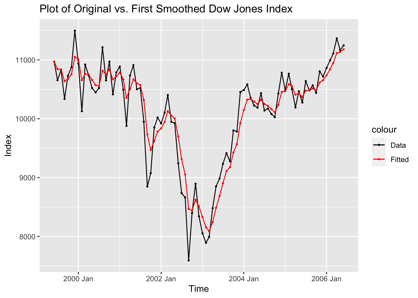
```
measacc.fs(dow_jones$index, 0.4)
```
```
## SSE MAPE MAD MSD
## 1.665968e+07 3.461342e+00 3.356325e+02 1.959962e+05
```
An alternative method of generating smoothed data is to use the `HoltWinters(data, alpha = , beta = , gamma = )` function, available through the `stats` package. `stats` is automatically included with R, so there is no need to call it. Since we are only doing simple exponential smoothing below, the `beta =` and `gamma =` parameters are set to `FALSE`. When the `alpha =`, `beta =`, and `gamma =` parameters are not specified, the optimal value of the parameter is calculated by minimizing the squared prediction error.
In the code chunk below, I calculate a simple exponential smoother when alpha = 0.4 and another simple exponential smoother where I let alpha be optimized. Then I plot the fitted values from both simple smoothers against the original data. Note: the `HoltWinters()` function fitted values contain one less observation than the original data. To plot it against the original data the first observation must be filtered out.
```
dj_smooth1 <- HoltWinters(dow_jones$index, alpha = 0.4, beta = FALSE, gamma = FALSE)
dj_smooth2 <- HoltWinters(dow_jones$index, beta = FALSE, gamma = FALSE)
dow_jones |>
filter(time != yearmonth("1999 Jun")) |>
ggplot(aes(x = time, y = index)) +
geom_point(aes(color = "Original"), size = 0.5) +
geom_line(aes(color = "Original")) +
geom_line(aes(y= dj_smooth1[["fitted"]][,1], color = "alpha = 0.4"), na.rm = TRUE) +
geom_point(aes(y= dj_smooth1[["fitted"]][,1], color = "alpha = 0.4"), size = 0.5, na.rm = TRUE) +
geom_line(aes(y= dj_smooth2[["fitted"]][,1], color = "alpha = 0.841"), na.rm = TRUE) +
geom_point(aes(y= dj_smooth2[["fitted"]][,1], color = "alpha = 0.841"), size = 0.5, na.rm = TRUE) +
scale_color_manual(values = c(Original = "black", "alpha = 0.4" = "red", "alpha = 0.841" = "blue")) +
labs(title = "Plot Dow Jones Index and First Smoothed Data",
x = "Time",
y = "Index",
color = "Data")
```
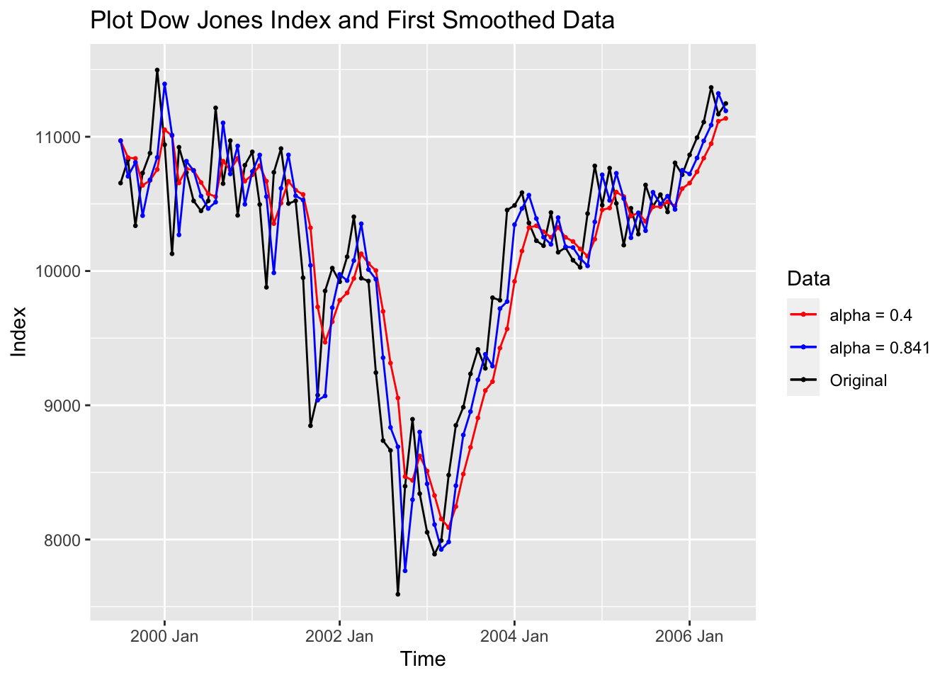
The `fpp3` packages use the same method of estimating exponential smoothing within model objects, but they use a different method to choose the initial value of the smoother. Instead of either setting the first value of the smoother to the first value of the series or the mean of the series, the `ETS()` function chooses the optimal value by minimizing SSE through log-likelihood. The optimization process can be changed using the `opt_crit =` parameter. The documentation for `ETS()` can be found [here](https://fable.tidyverts.org/reference/ETS.html). For further insight into `ETS()` and the equations for all the possible exponential smoothing model with this function, check out the tables at the bottom of [this page](https://otexts.com/fpp3/ets.html) as well as the rest of chapter 8.[34](https://bookdown.org/max_ricciardelli/forecasting_book/exponential-smoothing-methods.html#fn34) The simple exponential smoothing demonstrated below only has an error term (alpha parameter), so trend (beta) and season (gamma) are set to “N” signifying NULL. `alpha =` and `beta =` can both be set within the trend parameter and `gamma =` can be set within the season parameter.
```
dow_jones.fit <- dow_jones |>
model(model1 = ETS(index ~ error("A") + trend("N", alpha = 0.4) + season("N")),
model2 = ETS(index ~ error("A") + trend("N") + season("N")))
```
The table below contains both the alpha parameter and optimized starting value (l\[0\]) for both models. Additionally, I calculate the measures of accuracy for both models and compare them within the second table. The fable simple smoother optimization chooses an alpha parameter of 0.8494 instead of 0.841 chosen by the `HoltWinters()` function. Note: if the alpha parameter of the smoother is above 0.4, the smoother is not doing much smoothing.
```
dow_jones.fit |> tidy() |> mutate(estimate = round(estimate, digits = 3)) |> gt()
```
| .model | term | estimate |
|---|---|---|
| model1 | alpha | 0\.400 |
| model1 | l\[0\] | 10805\.637 |
| model2 | alpha | 0\.839 |
| model2 | l\[0\] | 10923\.490 |
```
dig <- function(x) (round(x, digits = 3))
dow_jones.fit |> accuracy() |> mutate_if(is.numeric, dig) |> gt()
```
| .model | .type | ME | RMSE | MAE | MPE | MAPE | MASE | RMSSE | ACF1 |
|---|---|---|---|---|---|---|---|---|---|
| model1 | Training | 11\.047 | 442\.152 | 336\.732 | \-0.074 | 3\.471 | 0\.391 | 0\.402 | 0\.434 |
| model2 | Training | 4\.423 | 400\.592 | 315\.600 | \-0.061 | 3\.208 | 0\.366 | 0\.364 | 0\.017 |
Finally, I analyze the residuals of each model using the `plot_residuals()` function.
```
augment(dow_jones.fit) |> filter(.model == "model1") |> plot_residuals()
```
```
## # A tibble: 1 × 3
## .model lb_stat lb_pvalue
## <chr> <dbl> <dbl>
## 1 model1 16.6 0.0000469
```
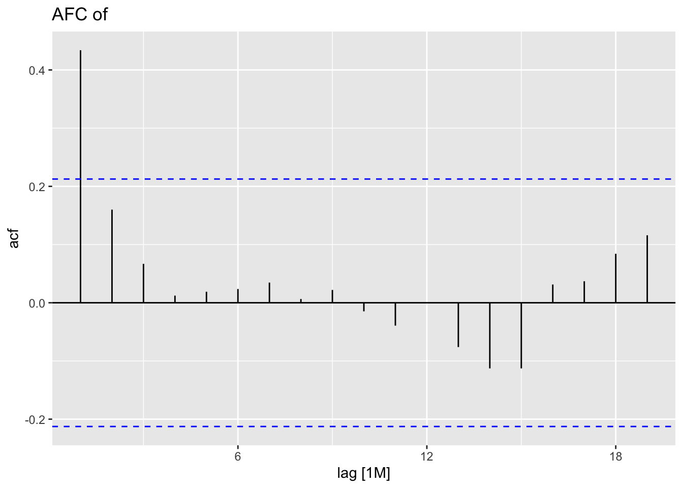
```
augment(dow_jones.fit) |> filter(.model == "model2") |> plot_residuals()
```
```
## # A tibble: 1 × 3
## .model lb_stat lb_pvalue
## <chr> <dbl> <dbl>
## 1 model2 0.0267 0.870
```
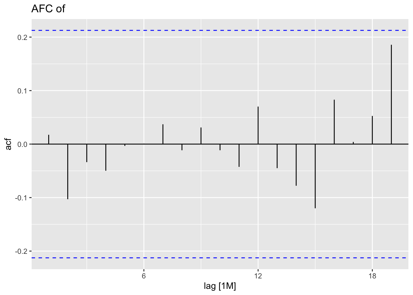
### 4\.10.3 Example 4.2: Double Exponential Smoothing
First, I read in the U.S. consumer price index data from US\_CPI.csv and create a tsibble object for it in the code chunk below. This data has issues with how time is kept, so it requires conditional formatting so the `yearmonth()` function can read it.
```
(cpi.data <- read_csv("data/US_CPI.csv") |>
rename("time" = 1, "index" = 2) |>
mutate(time = case_when(str_sub(time, start = 5, end = 5) == "9" ~ str_c("19",
str_sub(time, start = 5, end = 6),
"-",
str_sub(time, start = 1, end = 3)),
str_sub(time, start = 5, end = 5) == "0" ~ str_c("20",
str_sub(time, start = 5, end = 6),
"-", str_sub(time, start = 1, end = 3)))) |>
mutate(time = yearmonth(time)) |>
as_tsibble(index = time))
```
```
## Rows: 120 Columns: 2
## ── Column specification ───────────────────────────────────────
## Delimiter: ","
## chr (1): Month-Year
## dbl (1): CPI
##
## ℹ Use `spec()` to retrieve the full column specification for this data.
## ℹ Specify the column types or set `show_col_types = FALSE` to quiet this message.
```
```
## # A tsibble: 120 x 2 [1M]
## time index
## <mth> <dbl>
## 1 1995 Jan 150.
## 2 1995 Feb 151.
## 3 1995 Mar 151.
## 4 1995 Apr 152.
## 5 1995 May 152.
## 6 1995 Jun 152.
## 7 1995 Jul 152.
## 8 1995 Aug 153.
## 9 1995 Sep 153.
## 10 1995 Oct 154.
## # ℹ 110 more rows
```
After reading in the data appropriately, I calculate the first smoothed series and then the second smoothed series, both with a smoothing parameter of 0.3. Then, I calculate the predicted values by adjusting for bias.
```
cpi.smooth1 <- firstsmooth(y=cpi.data$index, lambda=0.3) # first order smoothing
cpi.smooth2 <- firstsmooth(y=cpi.smooth1, lambda=0.3) # second order smoothing
# take the first smoothed values as the y vector and choose the same lambda value
cpi.hat <- 2*cpi.smooth1 - cpi.smooth2 #Predicted value of y
# fitted value is twice the first smoother minus the second smoother
# these are the unbiased predicted values of y
```
I plot the original data, the predicted values, and the results of the first and second smoother all together in the code chunk below. The first and second smoother systematically underestimate the data, as seen in the plot.
```
cpi.data |>
ggplot(aes(x = time, y = index)) +
geom_point(aes(color = "Original"), size = 0.25) +
geom_line(aes(color = "Original")) +
geom_point(aes(y = cpi.hat, color = "Predicted Values"), size = 0.25) +
geom_line(aes(y = cpi.hat, color = "Predicted Values")) +
geom_point(aes(y = cpi.smooth1, color = "First Smoother"), size = 0.25) +
geom_line(aes(y = cpi.smooth1, color = "First Smoother")) +
geom_point(aes(y = cpi.smooth2, color = "Second Smoother"), size = 0.25) +
geom_line(aes(y = cpi.smooth2, color = "Second Smoother")) +
scale_color_manual(values = c(`Original` = "black",
`Predicted Values` = "red",
`First Smoother` = "blue",
`Second Smoother` = "green")) +
labs(title = "Plot of Original Data and Doubly Smoothed Fitted Values",
x = "Time",
y = "Index",
color = "Data")
```
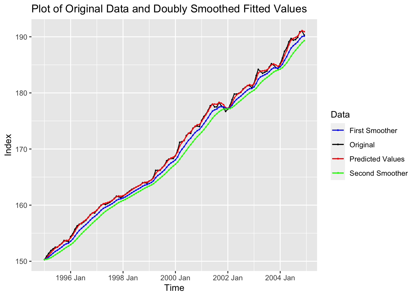
Next, I will replicate this using the methods from `fpp3`. I set both alpha and beta equal to 0.3 within `trend()`.
```
cpi.fit <- cpi.data |>
model(ETS(index ~ error("A") + trend("A", alpha = 0.3, beta = 0.3) + season("N")))
cpi.fit |> tidy() |> mutate(estimate = round(estimate, digits = 3)) |> gt()
```
| .model | term | estimate |
|---|---|---|
| ETS(index ~ error("A") + trend("A", alpha = 0.3, beta = 0.3) + season("N")) | alpha | 0\.300 |
| ETS(index ~ error("A") + trend("A", alpha = 0.3, beta = 0.3) + season("N")) | beta | 0\.300 |
| ETS(index ~ error("A") + trend("A", alpha = 0.3, beta = 0.3) + season("N")) | l\[0\] | 149\.952 |
| ETS(index ~ error("A") + trend("A", alpha = 0.3, beta = 0.3) + season("N")) | b\[0\] | 0\.628 |
```
augment(cpi.fit) |>
autoplot(index) +
geom_point(size = 0.25) +
autolayer(augment(cpi.fit), .fitted, color = "red") +
geom_point(aes(y = .fitted), color = "red", size = 0.25) +
labs(title = "Plot of CPI Index and Second Smoothed Data over Time",
subtitle = "Alpha = 0.3, Beta = 0.3",
x = "Time",
y = "Index")
```
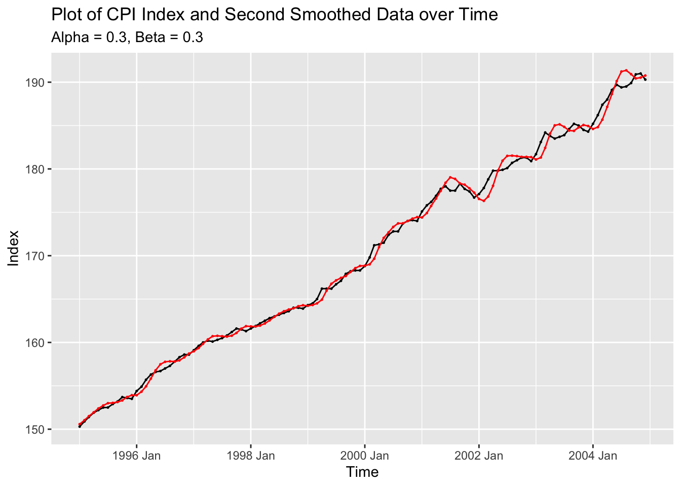
```
cpi.fit |> accuracy() |> mutate_if(is.numeric, dig) |> gt()
```
| .model | .type | ME | RMSE | MAE | MPE | MAPE | MASE | RMSSE | ACF1 |
|---|---|---|---|---|---|---|---|---|---|
| ETS(index ~ error("A") + trend("A", alpha = 0.3, beta = 0.3) + season("N")) | Training | \-0.019 | 0\.723 | 0\.535 | \-0.011 | 0\.306 | 0\.132 | 0\.171 | 0\.625 |
```
plot_residuals(augment(cpi.fit))
```
```
## # A tibble: 1 × 3
## .model lb_stat lb_pvalue
## <chr> <dbl> <dbl>
## 1 "ETS(index ~ error(\"A\") + trend(\"A\", alpha = 0.3, beta … 48.1 4.04e-12
```
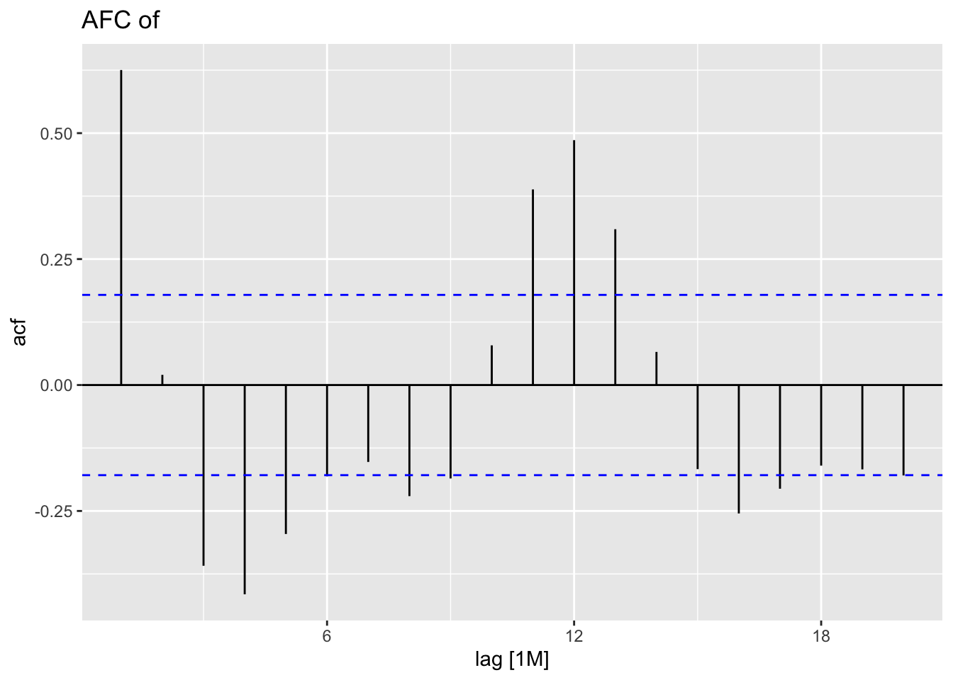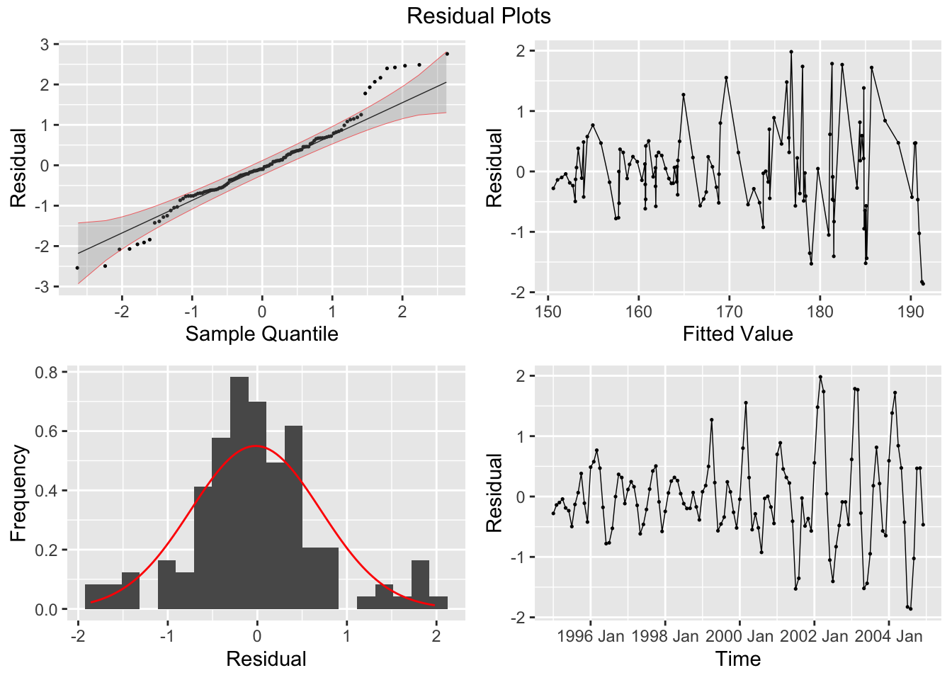
### 4\.10.4 Example 4.3: Double Exponential Smoothing
Next I will use the same double exponential smoothing procedure from the last example on the Dow Jones index data. In the code chunk below, I use the `firstsmooth()` custom function to doubly smooth the data and then calculate the fitted values.
```
dji.smooth3 <- firstsmooth(y=dow_jones$index, lambda=0.3) # first order smoothing
dji.smooth4 <- firstsmooth(y=dji.smooth3, lambda=0.3) # second order smoothing
dji.hat <- 2*dji.smooth3 - dji.smooth4 #Predicted value of y
# twice the first smoother minus the second smoother
```
Then, I plot the fitted values against the original data.
```
dow_jones |>
ggplot(aes(x = time, y = index)) +
geom_point(aes(color = "Original"), size = 0.5) +
geom_line(aes(color = "Original")) +
geom_point(aes(y = dji.hat, color ="Fitted"), size = 0.5) +
geom_line(aes(y = dji.hat, color = "Fitted")) +
scale_color_manual(values = c(Fitted = "red", Original = "black")) +
labs(title = "Plot of Dow Jones Index and Doubly Smoothed Data over Time",
subtitle = "alpha = 0.3, beta = 0.3",
x = "Time",
y = "Index",
color = "Data")
```

I then replicate this process using the methods from `fable` as done in the last example.
```
dow_jones.fit2 <- dow_jones |>
model(ETS(index ~ error("A") + trend("A", alpha = 0.3, beta = 0.3) + season("N")))
dow_jones.fit2 |> tidy() |> mutate(estimate = round(estimate, digits = 3)) |> gt()
```
| .model | term | estimate |
|---|---|---|
| ETS(index ~ error("A") + trend("A", alpha = 0.3, beta = 0.3) + season("N")) | alpha | 0\.300 |
| ETS(index ~ error("A") + trend("A", alpha = 0.3, beta = 0.3) + season("N")) | beta | 0\.300 |
| ETS(index ~ error("A") + trend("A", alpha = 0.3, beta = 0.3) + season("N")) | l\[0\] | 10608\.072 |
| ETS(index ~ error("A") + trend("A", alpha = 0.3, beta = 0.3) + season("N")) | b\[0\] | \-3.073 |
```
augment(dow_jones.fit2) |>
autoplot(index) +
geom_point(size = 0.25) +
autolayer(augment(dow_jones.fit2),.fitted, color = "red") +
geom_point(aes(y = .fitted), size = 0.25, color = "red") +
labs(title = "Plot of Dow Jones Index and Doubly Smoothed Data over Time",
subtitle = "Alpha = 0.3, Beta = 0.3",
x = "Time",
y = "Index")
```
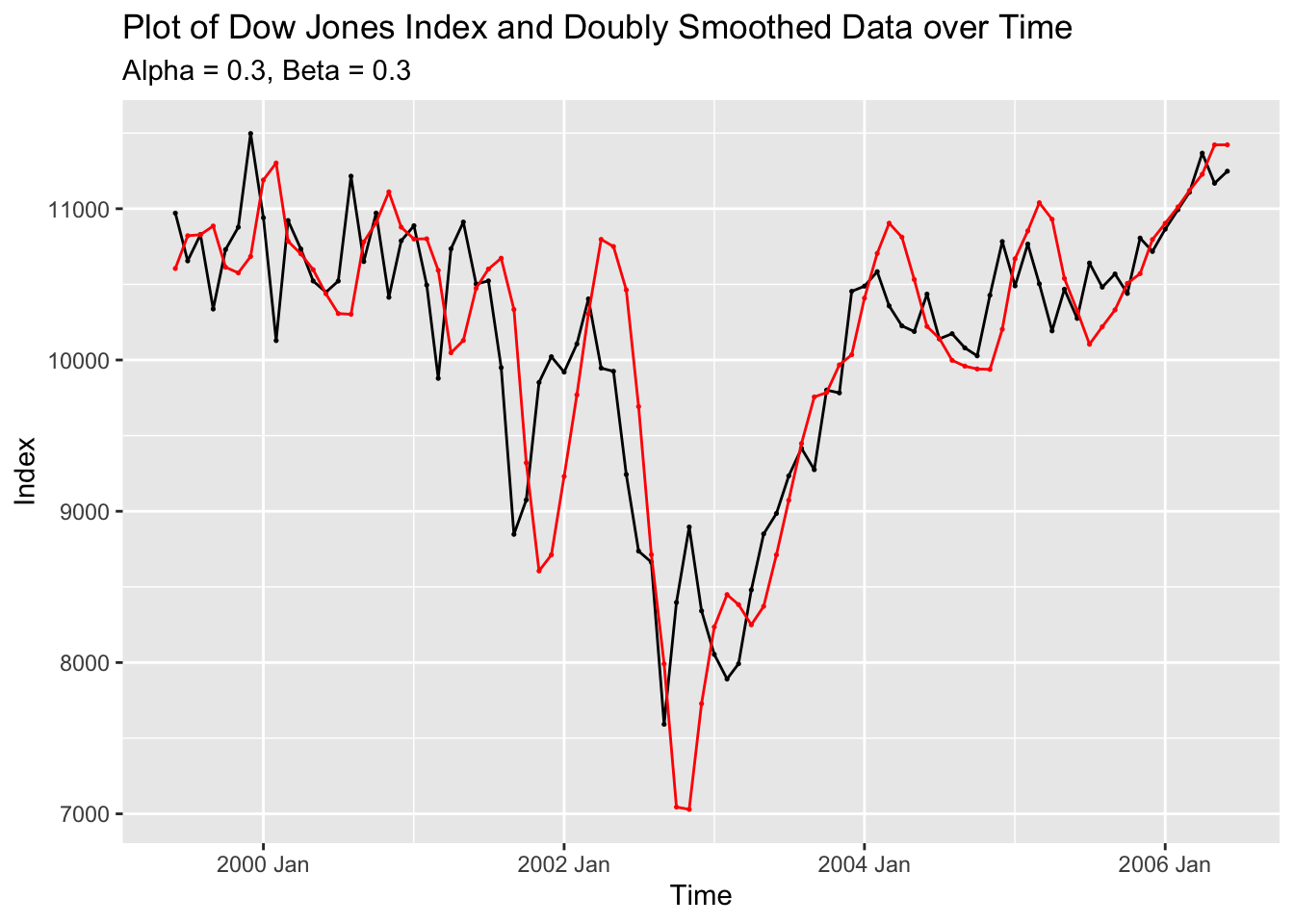
```
dow_jones.fit2 |> accuracy() |> mutate_if(is.numeric, dig) |> gt()
```
| .model | .type | ME | RMSE | MAE | MPE | MAPE | MASE | RMSSE | ACF1 |
|---|---|---|---|---|---|---|---|---|---|
| ETS(index ~ error("A") + trend("A", alpha = 0.3, beta = 0.3) + season("N")) | Training | 1\.065 | 556\.895 | 394\.388 | \-0.047 | 4\.04 | 0\.458 | 0\.506 | 0\.462 |
```
plot_residuals(augment(dow_jones.fit2))
```
```
## # A tibble: 1 × 3
## .model lb_stat lb_pvalue
## <chr> <dbl> <dbl>
## 1 "ETS(index ~ error(\"A\") + trend(\"A\", alpha = 0.3, beta … 18.8 0.0000148
```
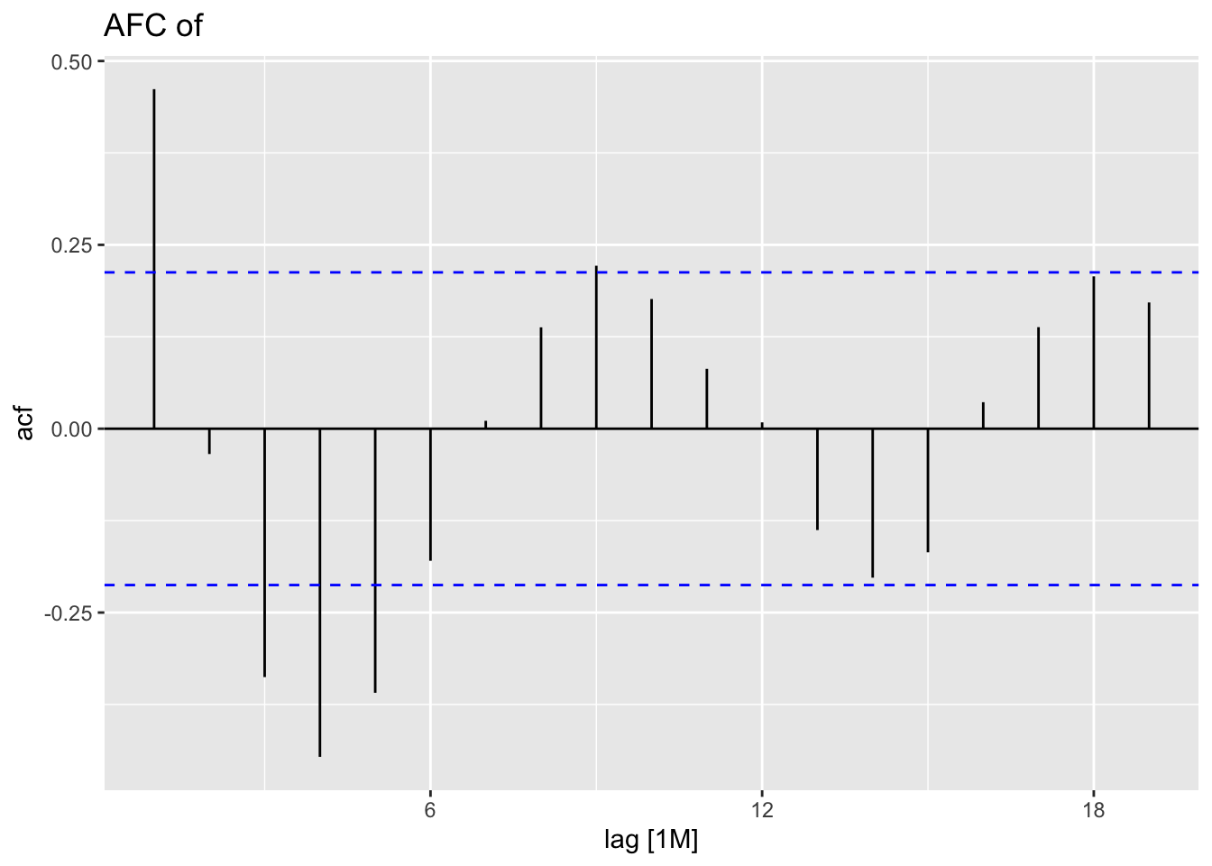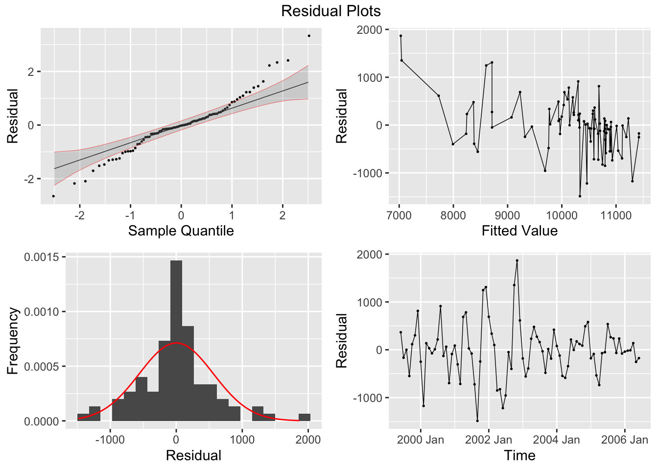
### 4\.10.5 Example 4.4: Forecasting a Constant Process
For this example, we will use the data from Speed.csv. This file contains the weekly average speed during non-rush hours.[35](https://bookdown.org/max_ricciardelli/forecasting_book/exponential-smoothing-methods.html#fn35) In the code chunk below, I read in the data and declare it as a tsibble.
```
(speed <- read_csv("data/Speed.csv") |>
rename(time = 1, speed = 2) |>
as_tsibble(index = time))
```
```
## Rows: 100 Columns: 2
## ── Column specification ───────────────────────────────────────
## Delimiter: ","
## dbl (2): Week, Speed
##
## ℹ Use `spec()` to retrieve the full column specification for this data.
## ℹ Specify the column types or set `show_col_types = FALSE` to quiet this message.
```
```
## # A tsibble: 100 x 2 [1]
## time speed
## <dbl> <dbl>
## 1 1 47.1
## 2 2 45.0
## 3 3 44.7
## 4 4 45.4
## 5 5 45.4
## 6 6 44.8
## 7 7 45.2
## 8 8 45.3
## 9 9 46.9
## 10 10 48.0
## # ℹ 90 more rows
```
I then manually calculate the optimal value of lambda and compare it to the results from the `HoltWinters()` function. We will use the first 78 values as the training set and the remaining 22 as the test set. I create a sequence of lambda values from 0.1 to 0.9 in increments of 0.1. Then, I write a custom function, `sse.speed`, that wraps `measacc.fs()`, and use the `sapply()` function to apply the sequence of lambdas to `sse.speed`. I then save the lambda with the smallest SSE to `opt.lambda`. I then graph each lambda and the resulting SSE, and denote the optimal lambda with a vertical red line. You can see that the optimal lambda is at the bottom of a parabola. `HoltWinters()` finds the optimal lambda to be 0.385.
```
lambda.vec <- seq(0.1, 0.9, 0.1) #Sequence of lambda values from 0.1 to 0.9 in increments of 0.1
# this uses the measures of accuracy function: only take the 1-78 observations and use the remaining ones as the holdout sample.
# The point is to use the 78 points to make the actual data and compare the forecasts to the remaining 22 points
sse.speed <- function(sc){measacc.fs(speed$speed[1:78], sc)[1]} #Apply "firstSmooth" through measacc
# holdout sample is important to monitor the forecast otherwise there is no measure of forecast performance
sse.vec <- sapply(lambda.vec, sse.speed) #SAPPLY instead of "for" loops for computational purpose
# this saves time in large data sets but functions in the same way
opt.lambda <- lambda.vec[sse.vec == min(sse.vec)] #Optimal lambda that minimizes SSE
tibble(lambda = lambda.vec,
sse = sse.vec) |>
ggplot(aes(x = lambda, y = sse)) +
geom_point() +
geom_line() +
geom_vline(aes(xintercept = opt.lambda), color = "red") +
labs(title = "SSE vs. Lambda",
subtitle = "SSE min = 116.69, Lambda = 0.4",
x = "Lambda",
y = "SSE")
```
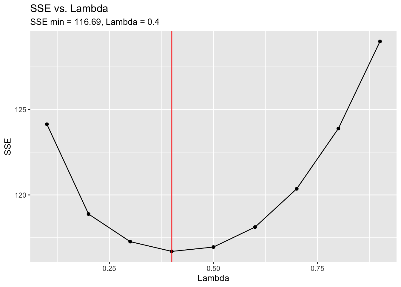
```
#Alternatively, use the Holt Winters function without specifying alpha parameter to get "best" value of smoothing constant.
(speed.hw <- HoltWinters(speed$speed, beta=FALSE, gamma=FALSE))
```
```
## Holt-Winters exponential smoothing without trend and without seasonal component.
##
## Call:
## HoltWinters(x = speed$speed, beta = FALSE, gamma = FALSE)
##
## Smoothing parameters:
## alpha: 0.3846525
## beta : FALSE
## gamma: FALSE
##
## Coefficients:
## [,1]
## a 45.61032
```
The methods in the `fable` package find the optimal alpha parameter to be 0.23. This differs due to the optimization of the first value of the smoother.
```
speed.fit <- speed |> filter(time <= 78) |>
model(ETS(speed ~ error("A") + trend("N") + season("N")))
speed.fit |> tidy() |> mutate(estimate = round(estimate, digits = 3)) |> gt()
```
| .model | term | estimate |
|---|---|---|
| ETS(speed ~ error("A") + trend("N") + season("N")) | alpha | 0\.00 |
| ETS(speed ~ error("A") + trend("N") + season("N")) | l\[0\] | 45\.45 |
```
accuracy(speed.fit) |> mutate_if(is.numeric, dig) |> gt()
```
| .model | .type | ME | RMSE | MAE | MPE | MAPE | MASE | RMSSE | ACF1 |
|---|---|---|---|---|---|---|---|---|---|
| ETS(speed ~ error("A") + trend("N") + season("N")) | Training | 0 | 1\.161 | 0\.919 | \-0.065 | 2\.016 | 0\.838 | 0\.874 | 0\.321 |
```
plot_residuals(augment(speed.fit))
```
```
## # A tibble: 1 × 3
## .model lb_stat lb_pvalue
## <chr> <dbl> <dbl>
## 1 "ETS(speed ~ error(\"A\") + trend(\"N\") + season(\"N\"))" 8.34 0.00388
```
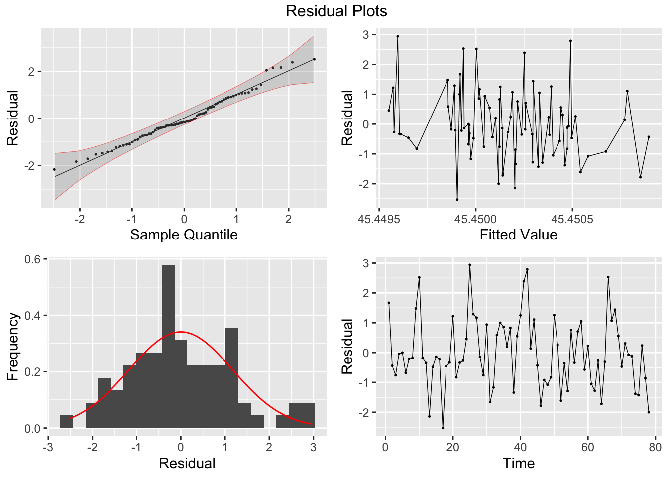
```
(speed.forecast <- speed.fit |> forecast(new_data = speed |> filter(time >= 79)))
```
```
## # A fable: 22 x 4 [1]
## # Key: .model [1]
## .model time speed .mean
## <chr> <dbl> <dist> <dbl>
## 1 "ETS(speed ~ error(\"A\") + trend(\"N\") + season(\"N… 79 N(45, 1.4) 45.4
## 2 "ETS(speed ~ error(\"A\") + trend(\"N\") + season(\"N… 80 N(45, 1.4) 45.4
## 3 "ETS(speed ~ error(\"A\") + trend(\"N\") + season(\"N… 81 N(45, 1.4) 45.4
## 4 "ETS(speed ~ error(\"A\") + trend(\"N\") + season(\"N… 82 N(45, 1.4) 45.4
## 5 "ETS(speed ~ error(\"A\") + trend(\"N\") + season(\"N… 83 N(45, 1.4) 45.4
## 6 "ETS(speed ~ error(\"A\") + trend(\"N\") + season(\"N… 84 N(45, 1.4) 45.4
## 7 "ETS(speed ~ error(\"A\") + trend(\"N\") + season(\"N… 85 N(45, 1.4) 45.4
## 8 "ETS(speed ~ error(\"A\") + trend(\"N\") + season(\"N… 86 N(45, 1.4) 45.4
## 9 "ETS(speed ~ error(\"A\") + trend(\"N\") + season(\"N… 87 N(45, 1.4) 45.4
## 10 "ETS(speed ~ error(\"A\") + trend(\"N\") + season(\"N… 88 N(45, 1.4) 45.4
## # ℹ 12 more rows
```
```
accuracy(speed.forecast, speed) |> mutate_if(is.numeric, dig) |> gt()
```
| .model | .type | ME | RMSE | MAE | MPE | MAPE | MASE | RMSSE | ACF1 |
|---|---|---|---|---|---|---|---|---|---|
| ETS(speed ~ error("A") + trend("N") + season("N")) | Test | \-0.334 | 0\.963 | 0\.825 | \-0.78 | 1\.834 | 0\.753 | 0\.725 | 0\.506 |
```
autoplot(speed.forecast, speed) +
labs(title = "Forecast of Mean Speed During Non-Rush Hours",
x = "Time",
y = "Speed")
```

### 4\.10.6 Example 4.5: Forecasting a Linear Trend Process
In this next example, we use the CPI data that was previously read in to forecast a linear trend process. We use simple exponential smoothing, optimizing the alpha parameter by minimizing the SSE. This is done using the same methods as the last example. The first 108 observations are used as the training set, while the final 12 are the test set.
```
# Finding the value of the smoothing constant that minimizes SSE using First-order exponential smoothing
lambda.vec <- c(seq(0.1, 0.9, 0.1), .95, .99) # series of possible lambda values
sse.cpi <- function(sc){measacc.fs(cpi.data$index[1:108],sc)[1]}
sse.vec <- sapply(lambda.vec, sse.cpi)
opt.lambda <- lambda.vec[sse.vec == min(sse.vec)]
tibble(lambda = lambda.vec,
sse = sse.vec) |>
ggplot(aes(x = lambda, y = sse)) +
geom_point() +
geom_line() +
geom_vline(aes(xintercept = opt.lambda), color = "red") +
labs(title = "SSE vs. Lambda",
subtitle = "SSE min = 28.65, Lambda = 1",
x = "Lambda",
y = "SSE")
```
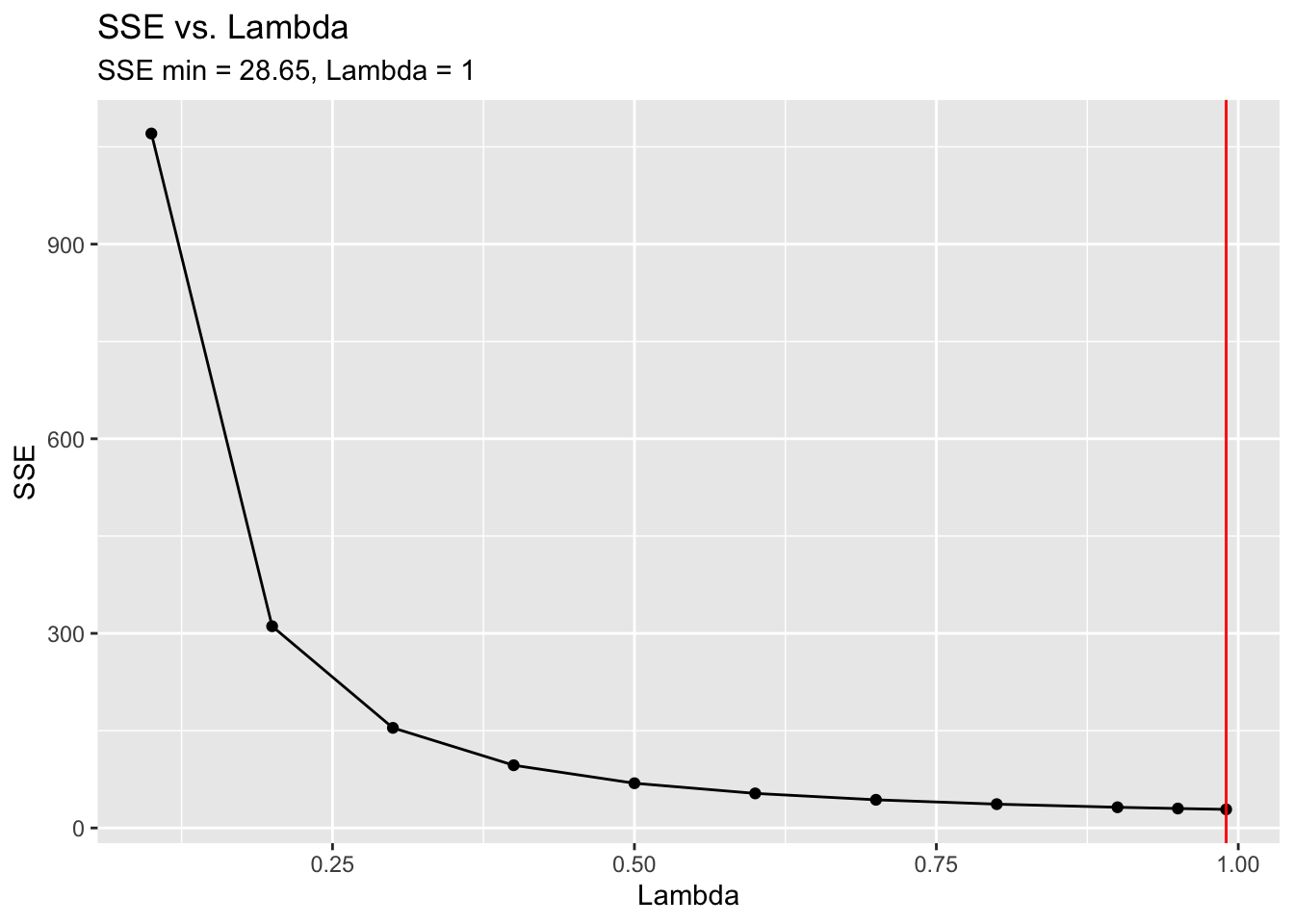
```
ACF(cpi.data |> filter(year(time) < 2004), index) |>
autoplot() +
labs(title = "ACF of CPI Data Training Set") #ACF of the data
```

#### 4\.10.6.1 Option A: 1 to 12 Step Ahead Forecast
I manually calculate a 1 to 12 step ahead forecast and read the results into a tibble.
```
#Now, we forecast using a Second-order exponential smoother with lambda=0.3
lcpi <- 0.3
cpi.smooth1 <- firstsmooth(y=cpi.data$index[1:108],lambda=lcpi)
cpi.smooth2 <- firstsmooth(y=cpi.smooth1, lambda=lcpi)
cpi.hat <- 2*cpi.smooth1 - cpi.smooth2
tau <- 1:12
T <- length(cpi.smooth1)
cpi.forecast <- (2 + tau*(lcpi/(1 - lcpi)))*cpi.smooth1[T] - (1+tau*(lcpi/(1-lcpi)))*cpi.smooth2[T]
# because we are saying tau it will do it for all values of tau
ctau <- sqrt(1 + (lcpi/((2-lcpi)^3))*(10-14*lcpi+5*(lcpi^2)+2*tau*lcpi*(4-3*lcpi)+2*(tau^2)*(lcpi^2)))
alpha.lev <- 0.05
sig.est <- sqrt(var(cpi.data$index[2:108] - cpi.hat[1:107]))
cl <- qnorm(1-alpha.lev/2)*(ctau/ctau[1])*sig.est
cpi.fc <- tibble(time = cpi.data$time[109:120],
mean = cpi.forecast,
upper = cpi.forecast + cl,
lower = cpi.forecast - cl)
```
Then I graph the forecast with the original data.
```
cpi.data |>
left_join(cpi.fc, by = join_by(time)) |>
ggplot(aes(x = time, y = index)) +
geom_point(size = 0.25) +
geom_line() +
geom_point(aes(y = mean), color = "blue", size = 0.25, na.rm = TRUE) +
geom_line(aes(y = mean), color = "blue", na.rm = TRUE) +
geom_ribbon(aes(ymax = upper, ymin = lower), fill = "blue", alpha = 0.5) +
labs(title = "1 to 12 Step-Ahead Forecast",
x = "Time",
y = "Index")
```
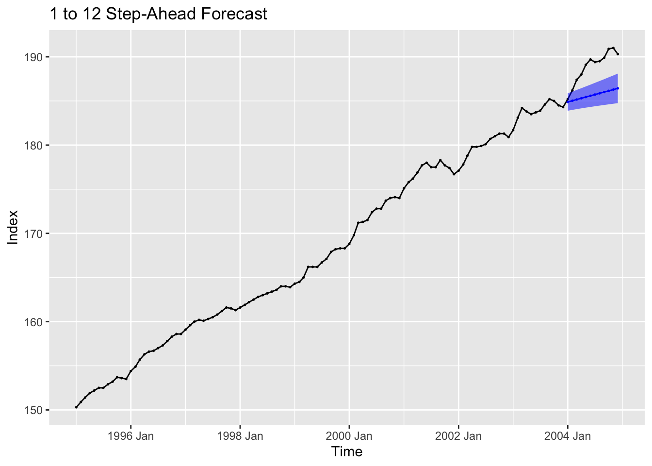
#### 4\.10.6.2 Option B: 12 One-Step-Ahead Forecasts
I then calculate 12 one-step ahead forecasts
```
lcpi <- 0.3
T <- 108
tau <- 12
alpha.lev <- 0.05
cpi.forecast <- rep(0,tau)
cl <- rep(0,tau)
cpi.smooth1 <- rep(0,T+tau)
cpi.smooth2 <- rep(0,T+tau)
for (i in 1:tau) {
cpi.smooth1[1:(T+i-1)] <- firstsmooth(y=cpi.data$index[1:(T+i-1)], lambda=lcpi)
cpi.smooth2[1:(T+i-1)] <- firstsmooth(y=cpi.smooth1[1:(T+i-1)], lambda=lcpi)
cpi.forecast[i] <- (2+(lcpi/(1-lcpi)))*cpi.smooth1[T+i-1]- (1+(lcpi/(1-lcpi)))*cpi.smooth2[T+i-1]
cpi.hat <- 2*cpi.smooth1[1:(T+i-1)] - cpi.smooth2[1:(T+i-1)]
sig.est <- sqrt(var(cpi.data[2:(T+i-1),2]- cpi.hat[1:(T+i-2)]))
cl[i] <- qnorm(1-alpha.lev/2)*sig.est
}
cpi.fc2 <- tibble(time = cpi.data$time[109:120],
mean = cpi.forecast,
upper = cpi.forecast + cl,
lower = cpi.forecast - cl)
```
I graph the results in the code chunk below.
```
cpi.data |>
left_join(cpi.fc2, by = join_by(time)) |>
ggplot(aes(x = time, y = index)) +
geom_point(size = 0.25) +
geom_line() +
geom_point(aes(y = mean), color = "blue", size = 0.25, na.rm = TRUE) +
geom_line(aes(y = mean), color = "blue", na.rm = TRUE) +
geom_ribbon(aes(ymax = upper, ymin = lower), fill = "blue", alpha = 0.5) +
labs(title = "12 One-Step-Ahead Forecast",
x = "Time",
y = "Index")
```
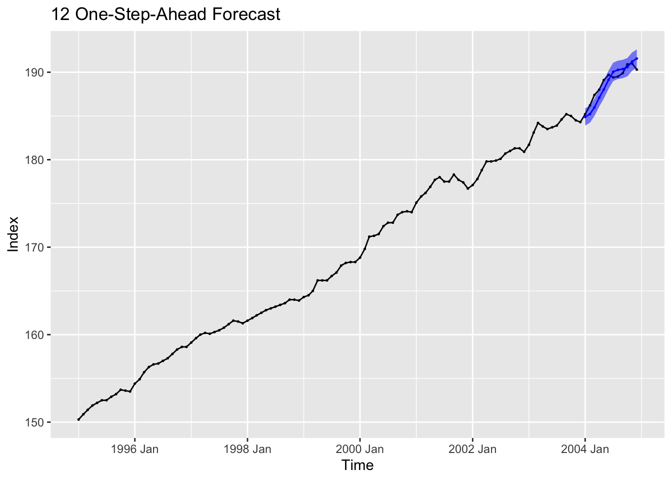
In fable, it is only possible to automatically do a 1 to 12 step ahead forecast. In the code chunk below, I estimate a 12 step ahead forecast using an analogous model in fable.
```
cpi.fit2 <- cpi.data |> filter(year(time) < 2004) |>
model(ETS(index ~ error("A") + trend("A", alpha = 0.3, beta = 0.3) + season("N")))
cpi.fit2 |> tidy() |> mutate(estimate = round(estimate, digits = 3)) |> gt()
```
| .model | term | estimate |
|---|---|---|
| ETS(index ~ error("A") + trend("A", alpha = 0.3, beta = 0.3) + season("N")) | alpha | 0\.300 |
| ETS(index ~ error("A") + trend("A", alpha = 0.3, beta = 0.3) + season("N")) | beta | 0\.300 |
| ETS(index ~ error("A") + trend("A", alpha = 0.3, beta = 0.3) + season("N")) | l\[0\] | 149\.952 |
| ETS(index ~ error("A") + trend("A", alpha = 0.3, beta = 0.3) + season("N")) | b\[0\] | 0\.628 |
```
cpi.fc3 <- cpi.fit2 |>
forecast(new_data = cpi.data |> filter(year(time) > 2003))
cpi.fc3 |> accuracy(cpi.data |> filter(year(time) > 2003)) |> mutate_if(is.numeric, dig) |> gt()
```
| .model | .type | ME | RMSE | MAE | MPE | MAPE | MASE | RMSSE | ACF1 |
|---|---|---|---|---|---|---|---|---|---|
| ETS(index ~ error("A") + trend("A", alpha = 0.3, beta = 0.3) + season("N")) | Test | 5\.075 | 5\.54 | 5\.075 | 2\.676 | 2\.676 | NaN | NaN | 0\.723 |
```
cpi.fc3 |>
autoplot(cpi.data)
```

To calculate 12 one-step-ahead forecasts using fable, I use a for loop to iteratively get all one step ahead forecasts for T+1 to T+tau. I then graph the results of this process against the test set.
```
one_step_for <- vector(mode = "list", length = 12) # create vectors to store the one step ahead forecasts
one_step_upper <- vector(mode = "list", length = 12)
one_step_lower <- vector(mode = "list", length = 12)
T <- 108 # define T
for (i in (T+1):(T+tau)){ # iterate 12 times, i = current period to forecast for
cpi.fit3 <- cpi.data[1:T,] |> # create a model with training data to one before i
model(ETS(index ~ error("A") + trend("A", alpha = 0.3, beta = 0.3) + season("N")))
cpi.forecast2 <- cpi.fit3 |> # create a one step ahead forecast
forecast(new_data = cpi.data[(T+1),])
one_step_for[i - 108] <- cpi.forecast2$.mean # record the mean
interval <- hilo(cpi.forecast2$index) # split the distribution into upper and lower bounds
one_step_upper[i - 108] <- interval$upper # record upper and lower
one_step_lower[i - 108] <- interval$lower
T <- T + 1 # update T
}
cpi.fc.tibble <- tibble(mean = one_step_for, # create a tibble containing mean and upper and lower bounds
lower = one_step_lower,
upper = one_step_upper) |>
mutate_all(as.numeric) |>
mutate(time = cpi.data$time[109:120])
cpi.data |> # plot the results
left_join(cpi.fc.tibble, by = join_by(time)) |>
ggplot(aes(x = time, y = index)) +
geom_point(size = 0.25) +
geom_line() +
geom_point(aes(y = mean), color = "blue", size = 0.25, na.rm = TRUE) +
geom_line(aes(y = mean), color = "blue", na.rm = TRUE) +
geom_ribbon(aes(ymin = lower, ymax = upper), fill = "blue", alpha = 0.5) +
labs(title = "12 One-Step Ahead Forecasts",
subtitle = "alpha = 0.3, beta = 0.3",
x = "Time",
y = "Index")
```
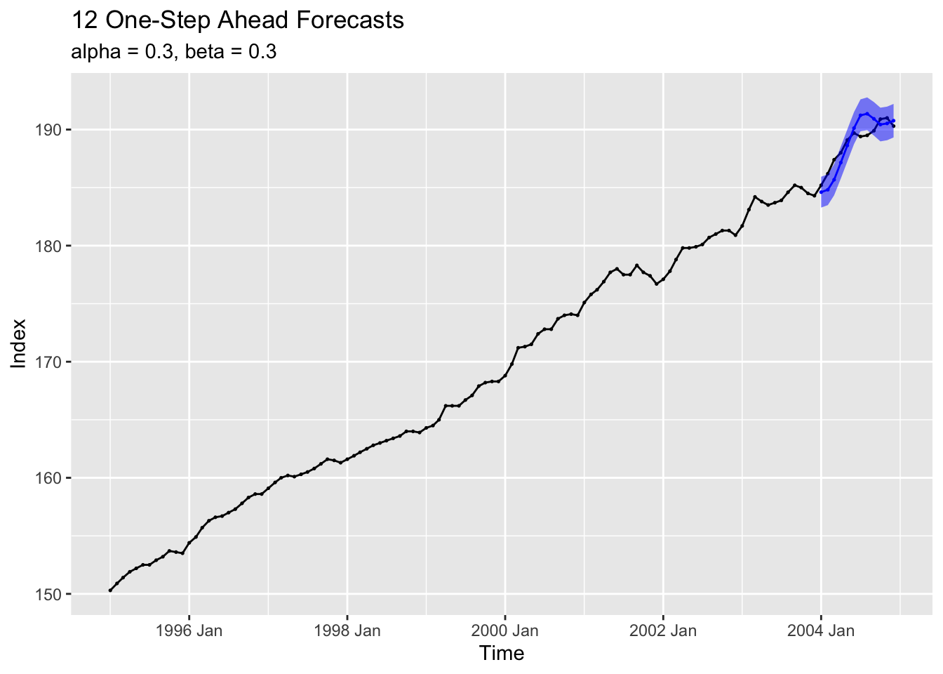
### 4\.10.7 Example 4.6: Adaptive Updating of the Discount Factor, Lambda
The Trigg-Leach method adaptively updates the discount factor. In the code chunk below, I define a custom function for the Trigg-Leach smoother.
```
#First, we define the Trigg-Leach Updating function:
tlsmooth<-function(y, gamma, y.tilde.start=y[1], lambda.start=1){
T <- length(y)
#Initialize the vectors
Qt <- vector()
Dt <- vector()
y.tilde <- vector()
lambda <- vector()
err <- vector()
#Set the starting values for the vectors
lambda[1] = lambda.start
y.tilde[1] = y.tilde.start
Qt[1] <- 0
Dt[1] <- 0
err[1] <- 0
for (i in 2:T){
err[i] <- y[i] - y.tilde[i-1]
Qt[i] <- gamma*err[i] + (1-gamma)*Qt[i-1]
Dt[i] <- gamma*abs(err[i]) + (1-gamma)*Dt[i-1]
lambda[i] <- abs(Qt[i]/Dt[i])
y.tilde[i] = lambda[i]*y[i] + (1-lambda[i])*y.tilde[i-1]
}
return(cbind(y.tilde, lambda, err, Qt, Dt))
}
```
Then, I run this function and `first_smooth()` on the dow\_jones data.
```
#Obtain the exponential smoother for Dow Jones Index
dji.smooth1 <- firstsmooth(y=dow_jones$index, lambda=0.4)
#Now, we apply the Trigg-Leach Smoothing function to the Dow Jones Index:
out.tl.dji <- tlsmooth(dow_jones$index, 0.3)
```
Plotting the results of both these methods with the original data, it is clear that the adaptive updating of the smoothing parameter leads to a better fit with this data.
```
#Plot the data together with TL and exponential smoother for comparison
dow_jones |>
ggplot(aes(x = time, y = index)) +
geom_point(aes(color = "Original Data"), size = 0.5) +
geom_line(aes(color = "Original Data")) +
geom_point(aes(y = dji.smooth1, color = "Simple Smooth"), size = 0.5) +
geom_line(aes(y = dji.smooth1, color = "Simple Smooth")) +
geom_point(aes(y = out.tl.dji[,1], color = "Trigg-Leach Smooth"), size = 0.5) +
geom_line(aes(y = out.tl.dji[,1], color = "Trigg-Leach Smooth")) +
scale_color_manual(values = c('Original Data' = "black",
"Simple Smooth" = "blue",
"Trigg-Leach Smooth" = "red")) +
labs(title = "Plot of Dow Jones, First Smoothed, and Trigg-Leach Smoothed Data",
x = "Time",
y = "Index")
```

This method only applies to a simple exponential smoother and is not included in the fable package, so it must be done using custom functions.
### 4\.10.8 Example 4.7: Exponential Smoothing for Additive Seasonal Model
In this section we will use clothing sales data contained in ClothingSales.csv.[36](https://bookdown.org/max_ricciardelli/forecasting_book/exponential-smoothing-methods.html#fn36) In the code chunk below, I read in the data and create a tsibble object to store it.
```
(clothing <- read_csv("data/ClothingSales.csv") |> mutate(year = case_when(
str_sub(Date, start = 5, end = 5) == "9" ~ str_c("19", str_sub(Date, start = 5, end = 6)),
substr(Date, 5, 5) == "0" ~ str_c("20", str_sub(Date, start = 5, end = 6)),
str_sub(Date, start = 1, end = 1) == "0" ~ str_c("20", str_sub(Date, start = 1, end = 2))
)) |>
mutate(month = case_when(str_sub(Date, 1, 1) == "0" ~ str_sub(Date, start = 4, end = 6),
str_sub(Date, 1, 1) != "0" ~ str_sub(Date, start = 1, end = 3)
)) |>
mutate(time = yearmonth(str_c(year,"-",month))) |>
select(time, Sales) |>
rename(sales = Sales) |>
as_tsibble(index = time))
```
```
## Rows: 144 Columns: 2
## ── Column specification ───────────────────────────────────────
## Delimiter: ","
## chr (1): Date
## dbl (1): Sales
##
## ℹ Use `spec()` to retrieve the full column specification for this data.
## ℹ Specify the column types or set `show_col_types = FALSE` to quiet this message.
```
```
## # A tsibble: 144 x 2 [1M]
## time sales
## <mth> <dbl>
## 1 1992 Jan 4889
## 2 1992 Feb 5197
## 3 1992 Mar 6061
## 4 1992 Apr 6720
## 5 1992 May 6811
## 6 1992 Jun 6579
## 7 1992 Jul 6598
## 8 1992 Aug 7536
## 9 1992 Sep 6923
## 10 1992 Oct 7566
## # ℹ 134 more rows
```
The holdout sample for this example is the first 132/144 observations. In the code chunk below, I use the `HoltWinters()` function to create an additive model where alpha = 0.2, beta. 0.2, and gamma = 0.2. I then plot that model against the original series and create forecasts, which I plot against the test sample.
```
clo.hw1 <- HoltWinters(clothing |> filter(year(time) < 2003), alpha=0.2, beta=0.2, gamma=0.2, seasonal="additive")
# create the additive model
# lose 12 observations
clothing |>
filter(year(time) < 2003 & year(time) > 1992) |> # filter data so it is the proper time frame
ggplot(aes(x = time, y = sales)) +
geom_point(aes(color = "Original"), size = 0.5) +
geom_line(aes(color = "Original")) +
geom_point(aes(y = clo.hw1[["fitted"]][,1], color = "Fitted"), size = 0.5) +
geom_line(aes(y = clo.hw1[["fitted"]][,1], color = "Fitted")) +
scale_color_manual(values = c("Fitted" = "red", "Original" = "black")) +
labs(title = "Clothing Sales Data Additive Seasonal Model",
subtitle = "Alpha = 0.2, Beta = 0.2, Gamma = 0.2",
x = "Time",
y = "Sales",
color = "Data")
```
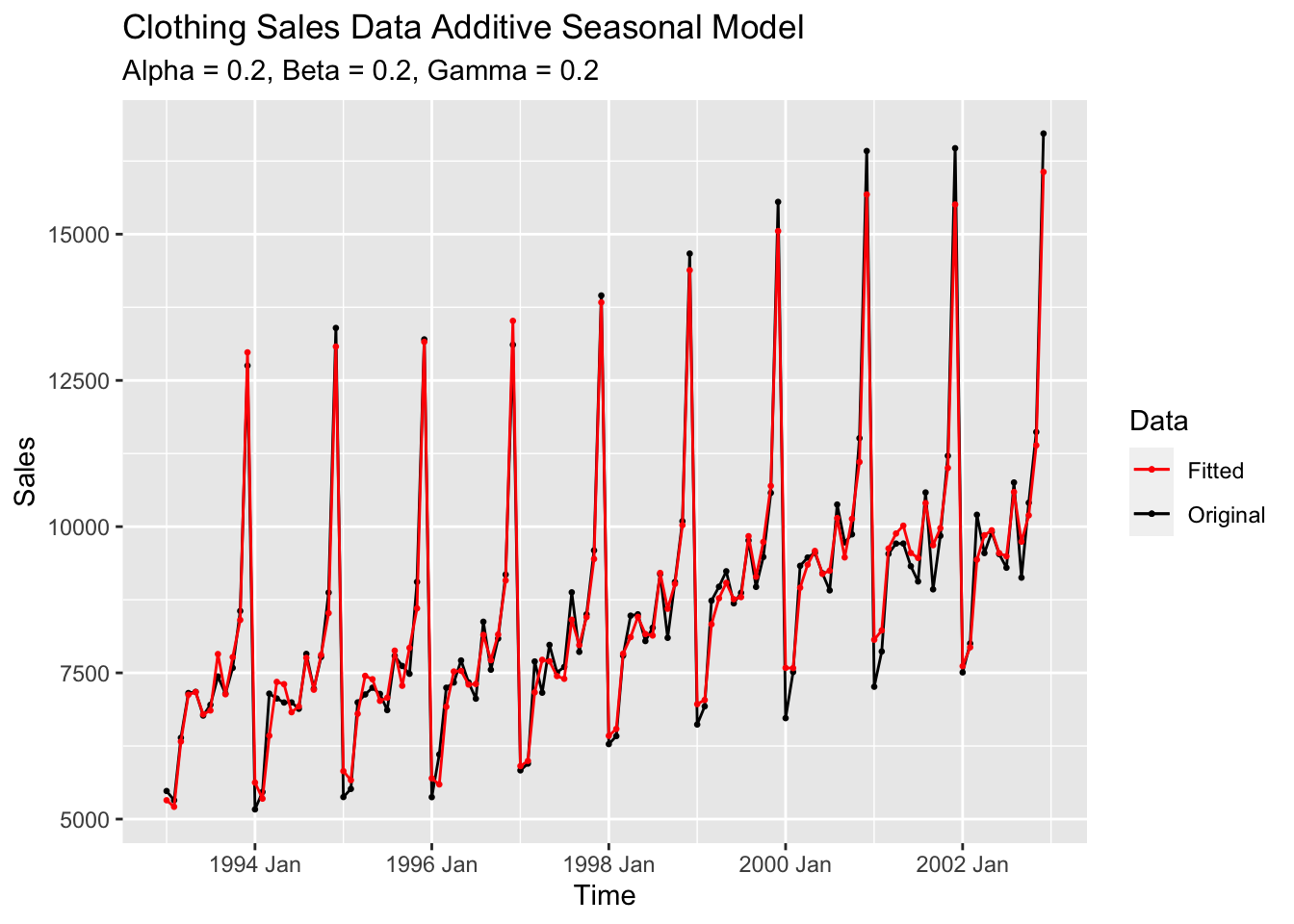
```
y2.forecast <- predict(clo.hw1, n.ahead=12, prediction.interval=TRUE)
# create forecasts
forecast <- tsibble(time = clothing$time[133:144],
fit = y2.forecast[,1],
upper = y2.forecast[,2],
lower = y2.forecast[,3],
index = time) # make tibble to store forecasts
clothing |>
left_join(forecast, by = join_by(time)) |> #join forecasts with data
ggplot(aes(x = time, y = sales)) +
geom_point(size = 0.5) +
geom_line() +
geom_line(aes(y = fit), color = "blue", na.rm = TRUE) +
geom_point(aes(y = fit), color = "blue", na.rm = TRUE) +
geom_ribbon(aes(ymin = lower, ymax = upper), fill = "blue", alpha = 0.5) +
labs(title = "Clothing Sales Data Additive Seasonal Model Forecast",
subtitle = "Alpha = 0.2, Beta = 0.2, Gamma = 0.2",
x = "Time",
y = "Sales")
```
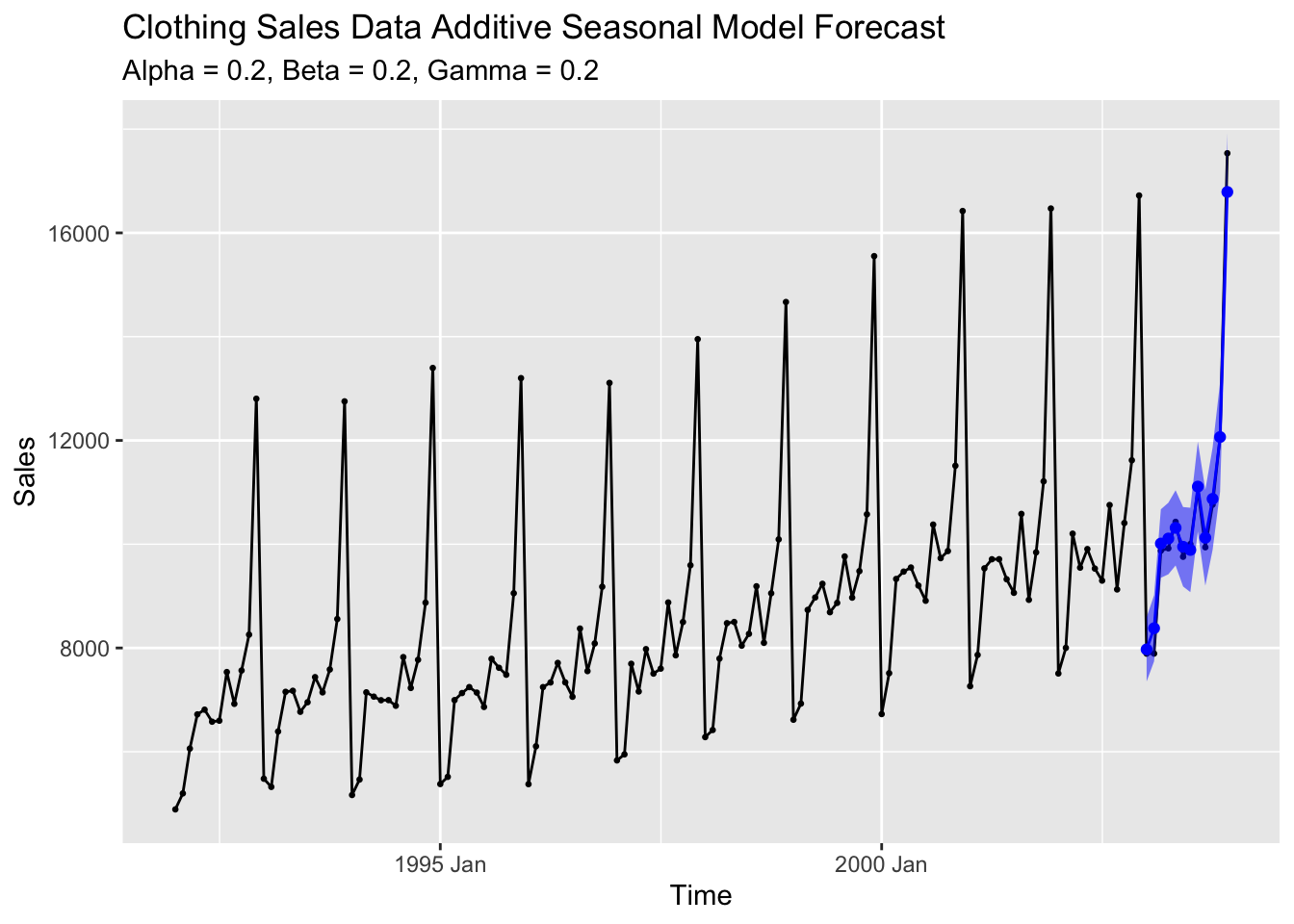
### 4\.10.9 Example 4.8: Exponential Smoothing for Multiplicative Seasonal Model
For this example we will use liquor sales data from LiquorSales.csv.[37](https://bookdown.org/max_ricciardelli/forecasting_book/exponential-smoothing-methods.html#fn37) In the code chunk below, I read in the data and create a tsibble object to store it.
```
(liquor <- read_csv("data/LiquorSales.csv") |>
mutate(year = case_when(
str_sub(Date, start = 5, end = 5) == "9" ~ str_c("19", str_sub(Date, start = 5, end = 6)),
substr(Date, 5, 5) == "0" ~ str_c("20", str_sub(Date, start = 5, end = 6)),
str_sub(Date, start = 1, end = 1) == "0" ~ str_c("20", str_sub(Date, start = 1, end = 2))
)) |>
mutate(month = case_when(str_sub(Date, 1, 1) == "0" ~ str_sub(Date, start = 4, end = 6),
str_sub(Date, 1, 1) != "0" ~ str_sub(Date, start = 1, end = 3)
)) |>
mutate(time = yearmonth(str_c(year,"-",month))) |>
select(time, Sales) |>
rename(sales = Sales) |>
as_tsibble(index = time))
```
```
## Rows: 156 Columns: 2
## ── Column specification ───────────────────────────────────────
## Delimiter: ","
## chr (1): Date
## dbl (1): Sales
##
## ℹ Use `spec()` to retrieve the full column specification for this data.
## ℹ Specify the column types or set `show_col_types = FALSE` to quiet this message.
```
```
## # A tsibble: 156 x 2 [1M]
## time sales
## <mth> <dbl>
## 1 1992 Jan 1519
## 2 1992 Feb 1551
## 3 1992 Mar 1606
## 4 1992 Apr 1686
## 5 1992 May 1834
## 6 1992 Jun 1786
## 7 1992 Jul 1924
## 8 1992 Aug 1874
## 9 1992 Sep 1781
## 10 1992 Oct 1894
## # ℹ 146 more rows
```
I then create an additive and multiplicative model of the whole data set, as well as a multiplicative model of just the holdout sample of the first 144 observations. I create 12 step-ahead forecasts for the model of the training set and put the results in a tibble.
```
liq.hw.add <- HoltWinters(liquor, alpha=0.2, beta=0.2, gamma=0.2, seasonal="additive")
liq.hw.mult<-HoltWinters(liquor, alpha=0.2, beta=0.2, gamma=0.2, seasonal="multiplicative")
liq.hw1 <- HoltWinters(liquor |> filter(year(time) < 2004), alpha=0.2, beta=0.2, gamma=0.2, seasonal="multiplicative")
y2.forecast <- predict(liq.hw1, n.ahead=12, prediction.interval = TRUE)
forecast2 <- tsibble(time = liquor$time[145:156],
fit = y2.forecast[,1],
upper = y2.forecast[,2],
lower = y2.forecast[,3],
index = time)
```
I then plot the additive and multiplicative model each in their own plots against the original data, and plot the forecasts against the test set.
```
liquor |>
filter(year(time) > 1992) |>
ggplot(aes(x = time, y = sales)) +
geom_point(aes(color = "Original Data"), size = 0.5) +
geom_line(aes(color = "Original Data")) +
geom_point(aes(y = liq.hw.add$fitted[,1], color = "Additive Model"), size = 0.5) +
geom_line(aes(y = liq.hw.add$fitted[,1], color = "Additive Model")) +
scale_color_manual(values = c("Original Data" = "black", "Additive Model" = "red")) +
labs(title = "Plot of Liquor Sales Data and Additive Model vs. Time",
x = "Time",
y = "Sales")
```

```
liquor |>
filter(year(time) > 1992) |>
ggplot(aes(x = time, y = sales)) +
geom_point(aes(color = "Original Data"), size = 0.5) +
geom_line(aes(color = "Original Data")) +
geom_point(aes(y = liq.hw.mult$fitted[,1], color = "Multiplicative Model"), size = 0.5) +
geom_line(aes(y = liq.hw.mult$fitted[,1], color = "Multiplicative Model")) +
scale_color_manual(values = c("Original Data" = "black", "Multiplicative Model" = "blue")) +
labs(title = "Plot of Liquor Sales Data and Multiplicative Model vs. Time",
x = "Time",
y = "Sales")
```
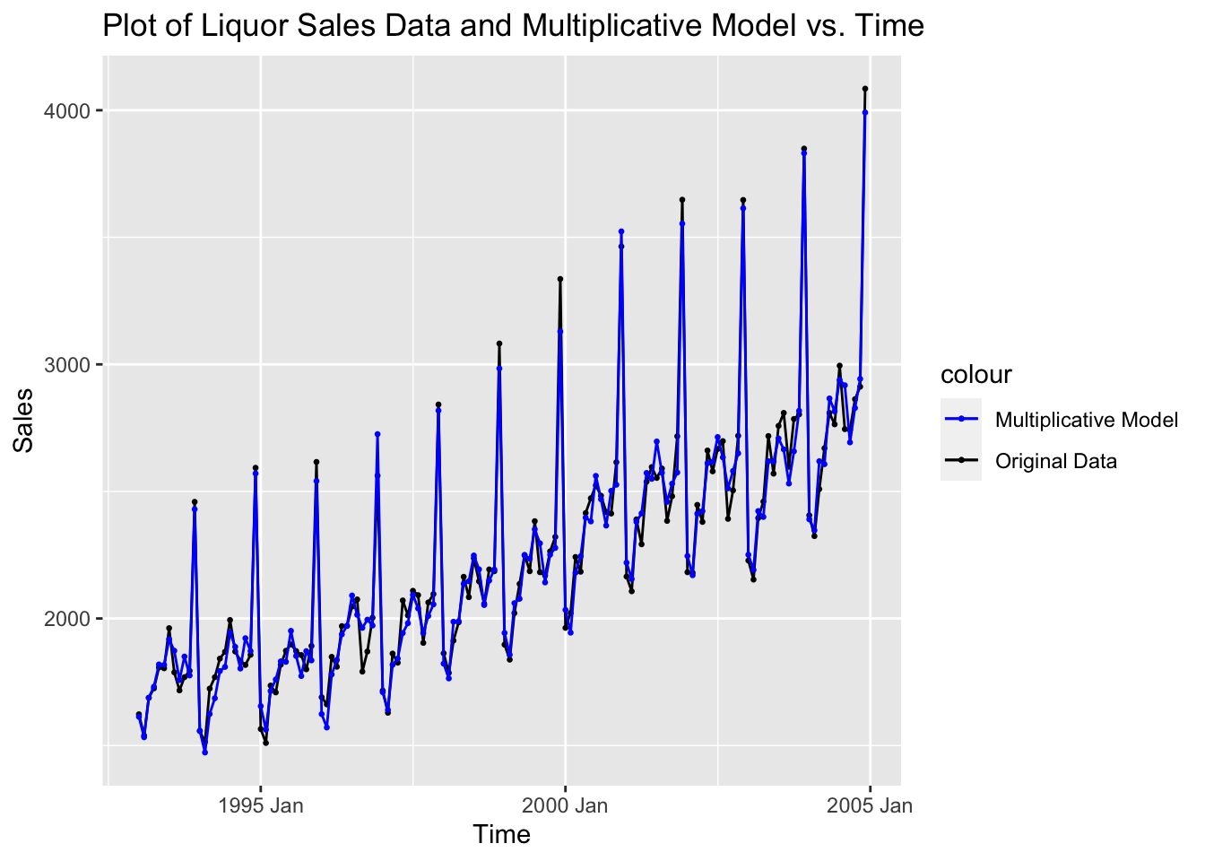
```
liquor |>
left_join(forecast2, by = join_by(time)) |>
ggplot(aes(x = time, y = sales)) +
geom_point(size = 0.5) +
geom_line() +
geom_line(aes(y = fit), color = "blue", na.rm = TRUE) +
geom_point(aes(y = fit), color = "blue", na.rm = TRUE) +
geom_ribbon(aes(ymin = lower, ymax = upper), fill = "blue", alpha = 0.5)
```
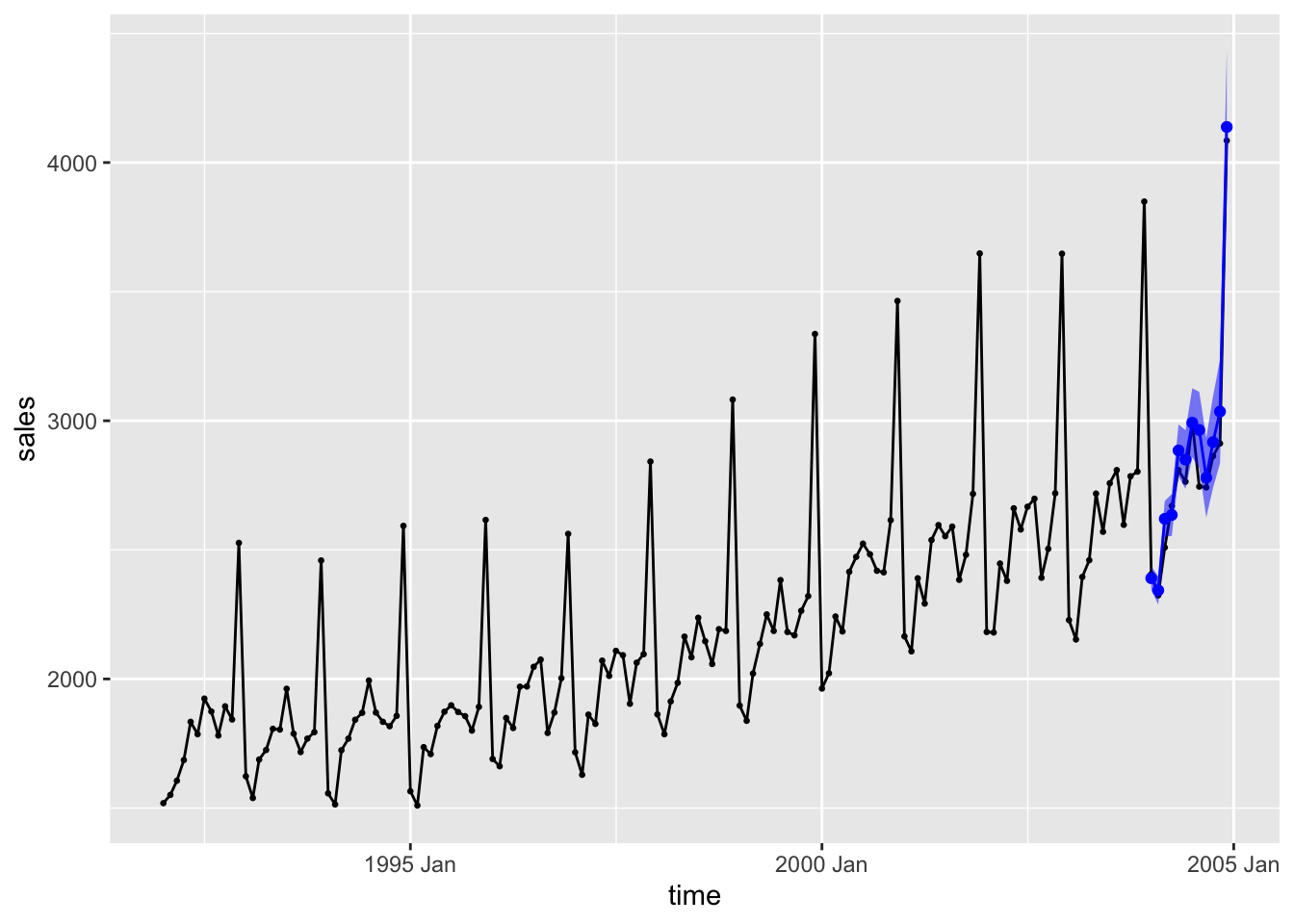
### 4\.10.10 Comparing an Additive and Multiplicative ETS Models
This section compares the possible ETS models within a single model object in `fable`. We use the liquor sales data from the last example as the data in this section. In the model object, I create three different models, an optimized model with all additive components, an optimized model with all multiplicative components, and a model that is the best model chosen from all possible `ETS()` models. The holdout sample will be all data before 2004 (1:144), and the test set will be the 2004 data (145:156).
```
liquor.fit <- liquor |>
filter(year(time) < 2004) |>
model(additive = ETS(sales ~ error("A") + trend("A") + season("A")),
multiplicative = ETS(sales ~ error("M") + trend("M") + season("M")),
opt = ETS(sales))
```
To compare the models at first glance, I use the custom function below to generate reports for each one.
```
gen_report <- function(models){
for (i in 1: length(models)){
print(colnames(models)[i])
report(models[i])
}
}
gen_report(liquor.fit)
```
```
## [1] "additive"
## Series: sales
## Model: ETS(A,A,A)
## Smoothing parameters:
## alpha = 0.3014984
## beta = 0.0001003563
## gamma = 0.6985013
##
## Initial states:
## l[0] b[0] s[0] s[-1] s[-2] s[-3] s[-4] s[-5]
## 1852.093 6.344784 835.0637 50.29692 -27.55822 -96.8937 32.12562 96.7324
## s[-6] s[-7] s[-8] s[-9] s[-10] s[-11]
## -2.986356 25.68023 -143.6287 -137.9088 -344.6557 -286.2675
##
## sigma^2: 5402.729
##
## AIC AICc BIC
## 1970.323 1975.180 2020.810
## [1] "multiplicative"
## Series: sales
## Model: ETS(M,M,M)
## Smoothing parameters:
## alpha = 0.2025417
## beta = 0.01421412
## gamma = 0.0001043186
##
## Initial states:
## l[0] b[0] s[0] s[-1] s[-2] s[-3] s[-4] s[-5]
## 1820.413 1.002463 1.387258 1.018877 0.9894544 0.9581219 1.019136 1.051209
## s[-6] s[-7] s[-8] s[-9] s[-10] s[-11]
## 0.9957197 1.012082 0.9332928 0.9313566 0.843961 0.8595313
##
## sigma^2: 8e-04
##
## AIC AICc BIC
## 1905.049 1909.906 1955.536
## [1] "opt"
## Series: sales
## Model: ETS(M,A,M)
## Smoothing parameters:
## alpha = 0.1975246
## beta = 0.01101548
## gamma = 0.0004288403
##
## Initial states:
## l[0] b[0] s[0] s[-1] s[-2] s[-3] s[-4] s[-5]
## 1819.605 0.4247737 1.38356 1.021844 0.991333 0.9542633 1.022034 1.046424
## s[-6] s[-7] s[-8] s[-9] s[-10] s[-11]
## 0.9957946 1.014296 0.9328883 0.9313987 0.8427128 0.8634506
##
## sigma^2: 8e-04
##
## AIC AICc BIC
## 1903.879 1908.736 1954.366
```
The completely optimized model has the lowest AIC, AICc, and BIC indicating that it has the most promise of the models we are evaluating. It uses multiplicative errors and seasonal components with an additive trend component. The both the multiplicative model and the optimal model have beta and gamma parameters close to zero, indicating that these components have little effect on the model as a whole. Next, I generate a table of the parameters of each model as well as a table of different measures of accuracy for each model.
```
liquor.fit |> tidy() |> mutate(estimate = round(estimate, digits = 3)) |> gt()
```
| .model | term | estimate |
|---|---|---|
| additive | alpha | 0\.301 |
| additive | beta | 0\.000 |
| additive | gamma | 0\.699 |
| additive | l\[0\] | 1852\.093 |
| additive | b\[0\] | 6\.345 |
| additive | s\[0\] | 835\.064 |
| additive | s\[-1\] | 50\.297 |
| additive | s\[-2\] | \-27.558 |
| additive | s\[-3\] | \-96.894 |
| additive | s\[-4\] | 32\.126 |
| additive | s\[-5\] | 96\.732 |
| additive | s\[-6\] | \-2.986 |
| additive | s\[-7\] | 25\.680 |
| additive | s\[-8\] | \-143.629 |
| additive | s\[-9\] | \-137.909 |
| additive | s\[-10\] | \-344.656 |
| additive | s\[-11\] | \-286.268 |
| multiplicative | alpha | 0\.203 |
| multiplicative | beta | 0\.014 |
| multiplicative | gamma | 0\.000 |
| multiplicative | l\[0\] | 1820\.413 |
| multiplicative | b\[0\] | 1\.002 |
| multiplicative | s\[0\] | 1\.387 |
| multiplicative | s\[-1\] | 1\.019 |
| multiplicative | s\[-2\] | 0\.989 |
| multiplicative | s\[-3\] | 0\.958 |
| multiplicative | s\[-4\] | 1\.019 |
| multiplicative | s\[-5\] | 1\.051 |
| multiplicative | s\[-6\] | 0\.996 |
| multiplicative | s\[-7\] | 1\.012 |
| multiplicative | s\[-8\] | 0\.933 |
| multiplicative | s\[-9\] | 0\.931 |
| multiplicative | s\[-10\] | 0\.844 |
| multiplicative | s\[-11\] | 0\.860 |
| opt | alpha | 0\.198 |
| opt | beta | 0\.011 |
| opt | gamma | 0\.000 |
| opt | l\[0\] | 1819\.605 |
| opt | b\[0\] | 0\.425 |
| opt | s\[0\] | 1\.384 |
| opt | s\[-1\] | 1\.022 |
| opt | s\[-2\] | 0\.991 |
| opt | s\[-3\] | 0\.954 |
| opt | s\[-4\] | 1\.022 |
| opt | s\[-5\] | 1\.046 |
| opt | s\[-6\] | 0\.996 |
| opt | s\[-7\] | 1\.014 |
| opt | s\[-8\] | 0\.933 |
| opt | s\[-9\] | 0\.931 |
| opt | s\[-10\] | 0\.843 |
| opt | s\[-11\] | 0\.863 |
```
liquor.fit |> accuracy() |> mutate_if(is.numeric, dig) |> gt()
```
| .model | .type | ME | RMSE | MAE | MPE | MAPE | MASE | RMSSE | ACF1 |
|---|---|---|---|---|---|---|---|---|---|
| additive | Training | 0\.262 | 69\.300 | 54\.351 | \-0.140 | 2\.530 | 0\.582 | 0\.594 | \-0.107 |
| multiplicative | Training | 1\.022 | 57\.165 | 45\.501 | \-0.012 | 2\.122 | 0\.487 | 0\.490 | \-0.005 |
| opt | Training | 5\.923 | 56\.727 | 45\.482 | 0\.218 | 2\.122 | 0\.487 | 0\.487 | \-0.014 |
The next step is to plot each model against the original series.
```
augment(liquor.fit |> select(additive)) |>
ggplot(aes(x = time, y = sales)) +
geom_point(aes(color = "Original"),size = 0.25) +
geom_line(aes(color = "Original")) +
geom_point(aes(y = .fitted, color = "Fitted"),size = 0.25) +
geom_line(aes(y = .fitted, color = "Fitted")) +
scale_color_manual(values = c("Fitted" = "red", "Original" = "black")) +
labs(title = "Plot of ETS(A,A,A) Model",
subtitle = "alpha = 0.301, beta = 0.000, gamma = 0.699",
color = "Data",
x = "Time",
y = "Sales")
```
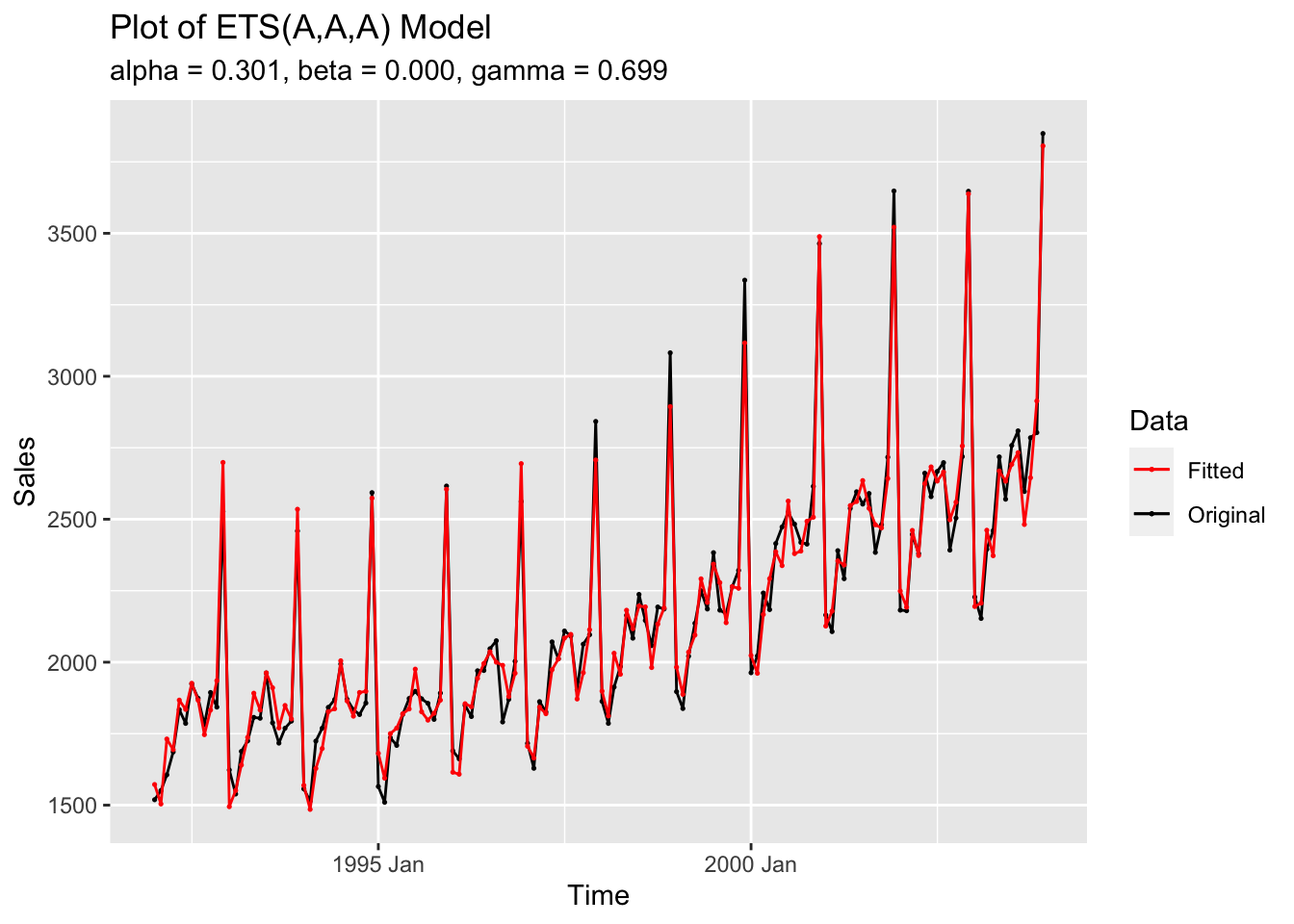
```
augment(liquor.fit |> select(multiplicative)) |>
ggplot(aes(x = time, y = sales)) +
geom_point(aes(color = "Original"),size = 0.25) +
geom_line(aes(color = "Original")) +
geom_point(aes(y = .fitted, color = "Fitted"),size = 0.25) +
geom_line(aes(y = .fitted, color = "Fitted")) +
scale_color_manual(values = c("Fitted" = "red", "Original" = "black")) +
labs(title = "Plot of ETS(M,M,M) Model",
subtitle = "alpha = 0.203, beta = 0.014, gamma = 0.000",
color = "Data",
x = "Time",
y = "Sales")
```

```
augment(liquor.fit |> select(opt)) |>
ggplot(aes(x = time, y = sales)) +
geom_point(aes(color = "Original"),size = 0.25) +
geom_line(aes(color = "Original")) +
geom_point(aes(y = .fitted, color = "Fitted"),size = 0.25) +
geom_line(aes(y = .fitted, color = "Fitted")) +
scale_color_manual(values = c("Fitted" = "red", "Original" = "black")) +
labs(title = "Plot of ETS(M,A,M) Model",
subtitle = "alpha = 0.198, beta = 0.011, gamma = 0.000",
color = "Data",
x = "Time",
y = "Sales")
```

Next, I plot the residuals for each model using `plot_residuals()`.
```
plot_residuals(augment(liquor.fit |> select(additive)), title = "ETS(A,A,A) Model")
```
```
## # A tibble: 1 × 3
## .model lb_stat lb_pvalue
## <chr> <dbl> <dbl>
## 1 additive 1.69 0.194
```
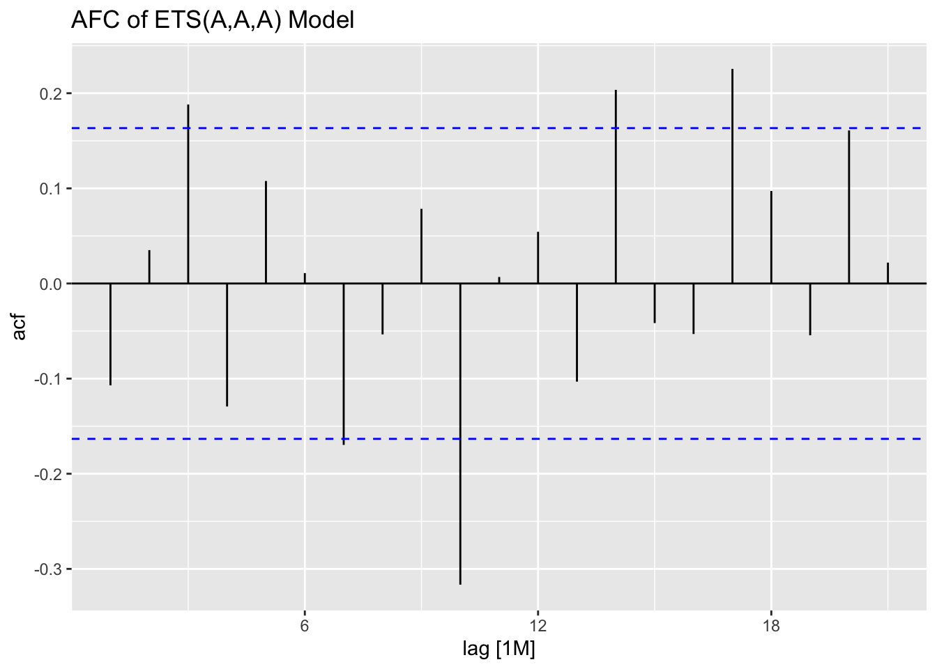
```
plot_residuals(augment(liquor.fit |> select(multiplicative)), title = "ETS(M,M,M) Model")
```
```
## # A tibble: 1 × 3
## .model lb_stat lb_pvalue
## <chr> <dbl> <dbl>
## 1 multiplicative 0.00391 0.950
```
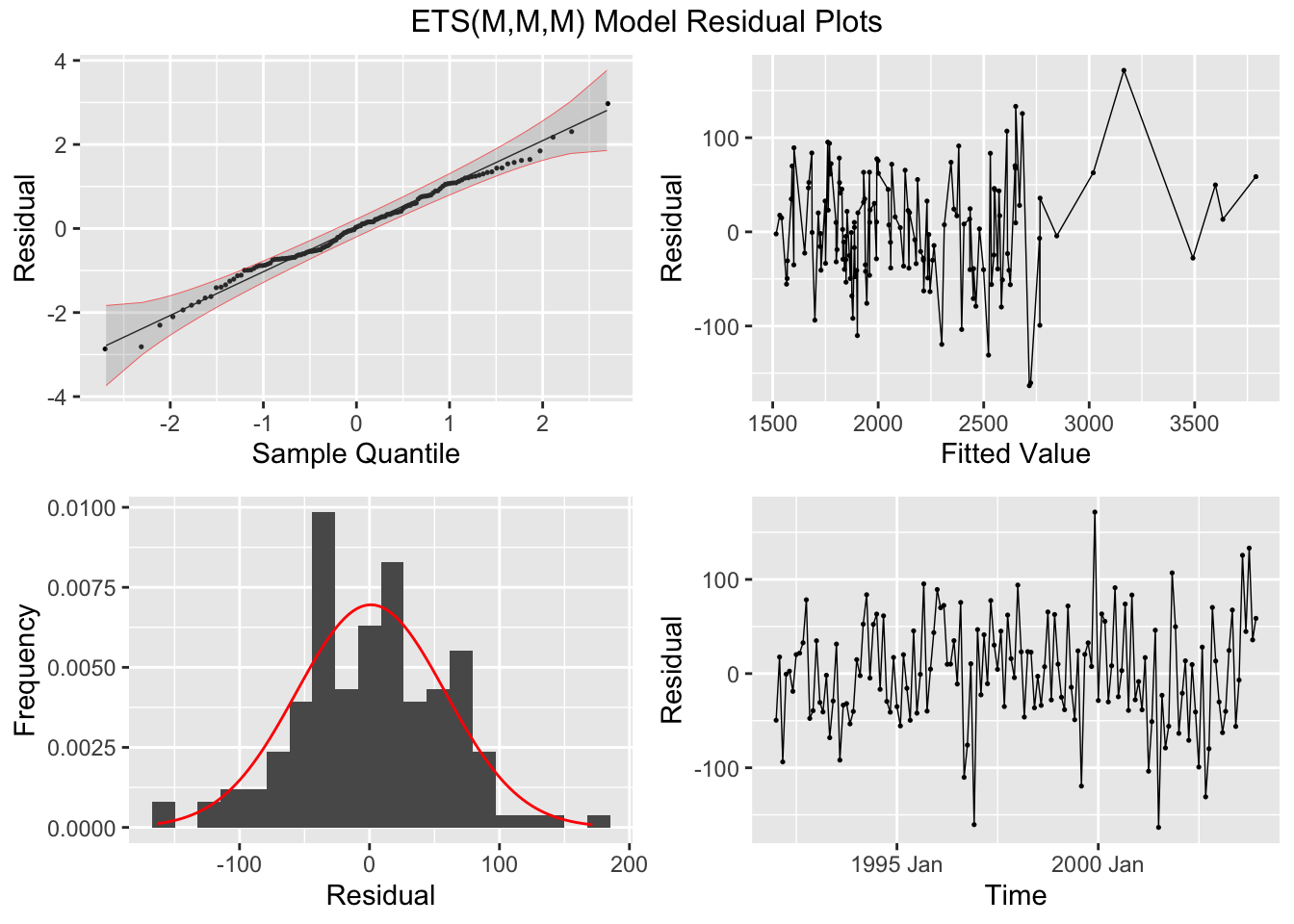
```
plot_residuals(augment(liquor.fit |> select(opt)), title = "ETS(M,A,M) Model")
```
```
## # A tibble: 1 × 3
## .model lb_stat lb_pvalue
## <chr> <dbl> <dbl>
## 1 opt 0.0304 0.861
```
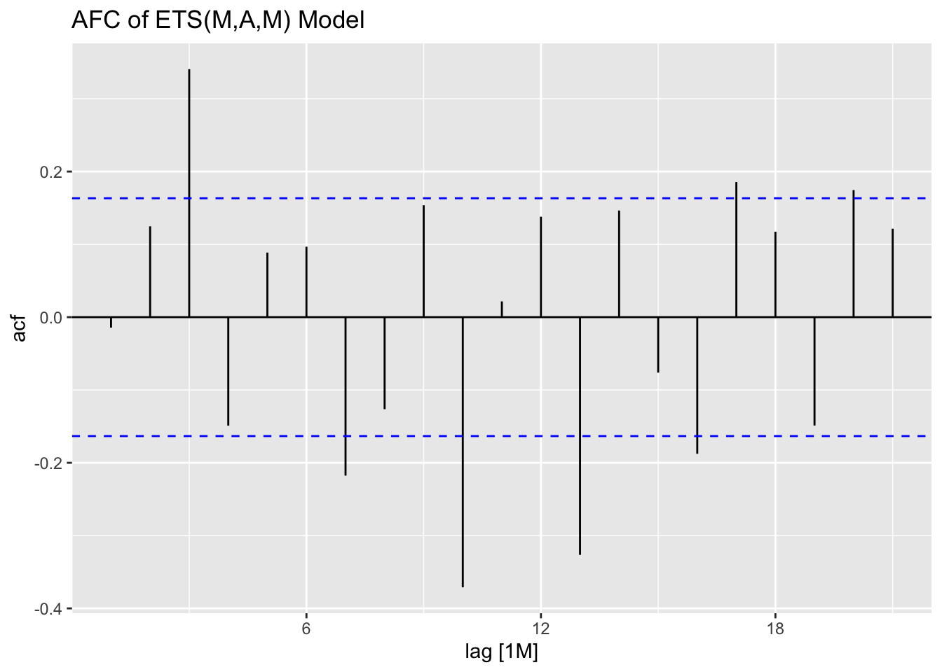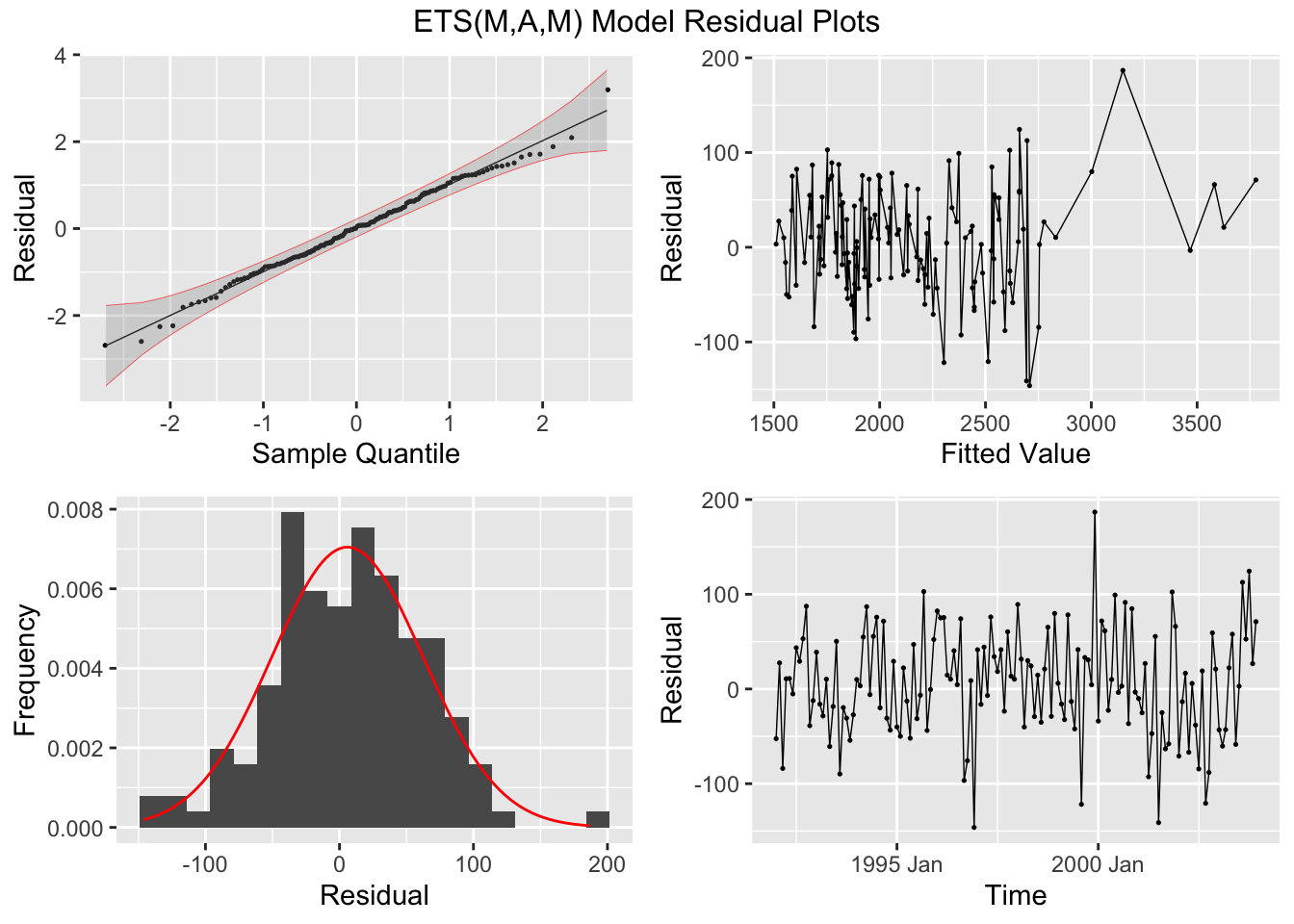
Then, I generate forecasts for each model, plot the forecasts for each model against each other, and make a table of the measure of accuracy for the test set. Looking at the results of the accuracy table, the. multiplicative model outperformed the other two, but all these models generate comparable forecasts.
```
liquor.fc <- forecast(liquor.fit, new_data = liquor |> filter(year(time) == 2004))
liquor.fc |> autoplot(liquor[145:156,]) + facet_wrap(~.model)
```
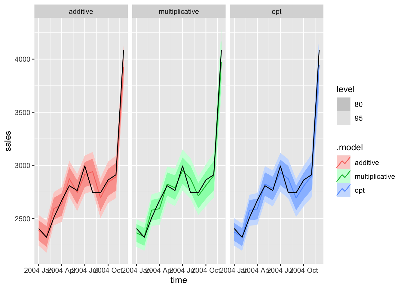
```
accuracy(liquor.fc, liquor) |> mutate_if(is.numeric, dig) |> gt()
```
| .model | .type | ME | RMSE | MAE | MPE | MAPE | MASE | RMSSE | ACF1 |
|---|---|---|---|---|---|---|---|---|---|
| additive | Test | 4\.141 | 85\.361 | 63\.019 | \-0.048 | 2\.143 | 0\.675 | 0\.732 | \-0.288 |
| multiplicative | Test | 9\.641 | 63\.457 | 50\.456 | 0\.223 | 1\.752 | 0\.540 | 0\.544 | \-0.280 |
| opt | Test | 16\.428 | 70\.465 | 55\.576 | 0\.433 | 1\.897 | 0\.595 | 0\.604 | \-0.315 |
### References
Hyndman, Rob J, and George Athanasopoulos. *Forecasting Principles and Practice*. Vol. 3. Melbourne, Australia: OTexts, 2021.
Montgomery, Douglas C, Cheryl L. Jennings, and Murat Kulahci. *Introduction to Time Series Analysis and Forecasting*. Vol. 2. Hoboken, New Jersey: John Wiley & Sons, 2016.
***
1. [Montgomery, Jennings, and Kulahci](https://bookdown.org/max_ricciardelli/forecasting_book/exponential-smoothing-methods.html#ref-forecasting).[↩︎](https://bookdown.org/max_ricciardelli/forecasting_book/exponential-smoothing-methods.html#fnref32)
2. [Montgomery, Jennings, and Kulahci](https://bookdown.org/max_ricciardelli/forecasting_book/exponential-smoothing-methods.html#ref-forecasting).[↩︎](https://bookdown.org/max_ricciardelli/forecasting_book/exponential-smoothing-methods.html#fnref33)
3. [Hyndman and Athanasopoulos, *Forecasting Principles and Practice*](https://bookdown.org/max_ricciardelli/forecasting_book/exponential-smoothing-methods.html#ref-fpp3).[↩︎](https://bookdown.org/max_ricciardelli/forecasting_book/exponential-smoothing-methods.html#fnref34)
4. [Montgomery, Jennings, and Kulahci, *Introduction to Time Series Analysis and Forecasting*](https://bookdown.org/max_ricciardelli/forecasting_book/exponential-smoothing-methods.html#ref-forecasting).[↩︎](https://bookdown.org/max_ricciardelli/forecasting_book/exponential-smoothing-methods.html#fnref35)
5. [Montgomery, Jennings, and Kulahci](https://bookdown.org/max_ricciardelli/forecasting_book/exponential-smoothing-methods.html#ref-forecasting).[↩︎](https://bookdown.org/max_ricciardelli/forecasting_book/exponential-smoothing-methods.html#fnref36)
6. [Montgomery, Jennings, and Kulahci](https://bookdown.org/max_ricciardelli/forecasting_book/exponential-smoothing-methods.html#ref-forecasting).[↩︎](https://bookdown.org/max_ricciardelli/forecasting_book/exponential-smoothing-methods.html#fnref37) | |||||||||||||||
| Readable Markdown | null | |||||||||||||||
| ML Classification | ||||||||||||||||
| ML Categories |
Raw JSON{
"/Science": 673,
"/Science/Mathematics": 551,
"/Science/Mathematics/Statistics": 537,
"/Computers_and_Electronics": 204,
"/Computers_and_Electronics/Software": 128
} | |||||||||||||||
| ML Page Types |
Raw JSON{
"/Article": 781,
"/Article/Tutorial_or_Guide": 766
} | |||||||||||||||
| ML Intent Types |
Raw JSON{
"Informational": 999
} | |||||||||||||||
| Content Metadata | ||||||||||||||||
| Language | null | |||||||||||||||
| Author | Jaya Jha | |||||||||||||||
| Publish Time | 2023-10-26 00:00:00 (2 years ago) | |||||||||||||||
| Original Publish Time | 2023-09-07 20:10:32 (2 years ago) | |||||||||||||||
| Republished | Yes | |||||||||||||||
| Word Count (Total) | 12,412 | |||||||||||||||
| Word Count (Content) | 11,735 | |||||||||||||||
| Links | ||||||||||||||||
| External Links | 2 | |||||||||||||||
| Internal Links | 9 | |||||||||||||||
| Technical SEO | ||||||||||||||||
| Meta Nofollow | No | |||||||||||||||
| Meta Noarchive | No | |||||||||||||||
| JS Rendered | No | |||||||||||||||
| Redirect Target | null | |||||||||||||||
| Performance | ||||||||||||||||
| Download Time (ms) | 125 | |||||||||||||||
| TTFB (ms) | 50 | |||||||||||||||
| Download Size (bytes) | 412,966 | |||||||||||||||
| Shard | 39 (laksa) | |||||||||||||||
| Root Hash | 3646282709075601439 | |||||||||||||||
| Unparsed URL | org,bookdown!/max_ricciardelli/forecasting_book/exponential-smoothing-methods.html s443 | |||||||||||||||