ℹ️ Skipped - page is already crawled
| Filter | Status | Condition | Details |
|---|---|---|---|
| HTTP status | PASS | download_http_code = 200 | HTTP 200 |
| Age cutoff | PASS | download_stamp > now() - 6 MONTH | 0 months ago |
| History drop | PASS | isNull(history_drop_reason) | No drop reason |
| Spam/ban | PASS | fh_dont_index != 1 AND ml_spam_score = 0 | ml_spam_score=0 |
| Canonical | PASS | meta_canonical IS NULL OR = '' OR = src_unparsed | Not set |
| Property | Value | |||||||||||||||
|---|---|---|---|---|---|---|---|---|---|---|---|---|---|---|---|---|
| URL | https://aosmith.rbind.io/2019/03/06/lots-of-zeros/ | |||||||||||||||
| Last Crawled | 2026-04-28 01:18:37 (13 hours ago) | |||||||||||||||
| First Indexed | 2019-03-06 20:37:57 (7 years ago) | |||||||||||||||
| HTTP Status Code | 200 | |||||||||||||||
| Content | ||||||||||||||||
| Meta Title | Lots of zeros or too many zeros?: Thinking about zero inflation in count data | |||||||||||||||
| Meta Description | When working with counts, having many zeros does not necessarily indicate zero inflation. I demonstrate this by simulating data from the negative binomial and generalized Poisson distributions. I then show one way to check if the data has excess zeros compared to the number of zeros expected based on the model. | |||||||||||||||
| Meta Canonical | null | |||||||||||||||
| Boilerpipe Text | In a recent lecture I gave a basic overview of zero-inflation in count distributions. My main take-home message to the students that I thought worth posting about here is that having a lot of zero values does not necessarily mean you have zero inflation.
Zero inflation is when there are more 0 values in the data than the distribution allows for. But some distributions can have a lot of zeros!
Table of Contents
Load packages and dataset
Negative binomial with many zeros
Generalized Poisson with many zeros
Lots of zeros or excess zeros?
Simulate negative binomial data
Checking for excess zeros
An example with excess zeros
Just the code, please
Load packages and dataset
I’m going to be simulating counts from different distributions to demonstrate this. First I’ll load the packages I’m using today.
Package
HMMpa
is for a function to draw random samples from the generalized Poisson distribution.
library(ggplot2) # v. 3.1.0
library(HMMpa) # v. 1.0.1
library(MASS) # v. 7.3-51.1
Negative binomial with many zeros
First I’ll draw 200 counts from a negative binomial with a mean (
\(\lambda\)
) of
\(10\)
and
\(\theta = 0.05\)
.
R uses the parameterization of the negative binomial where the variance of the distribution is
\(\lambda + (\lambda^2/\theta)\)
. In this parameterization, as
\(\theta\)
gets small the variance gets big. Using a very small value of theta like I am will generally mean the distribution of counts will have many zeros as well as a few large counts
I pull a random sample of size 200 from this distribution using
rnbinom()
. The
mu
argument is the mean and the
size
argument is theta.
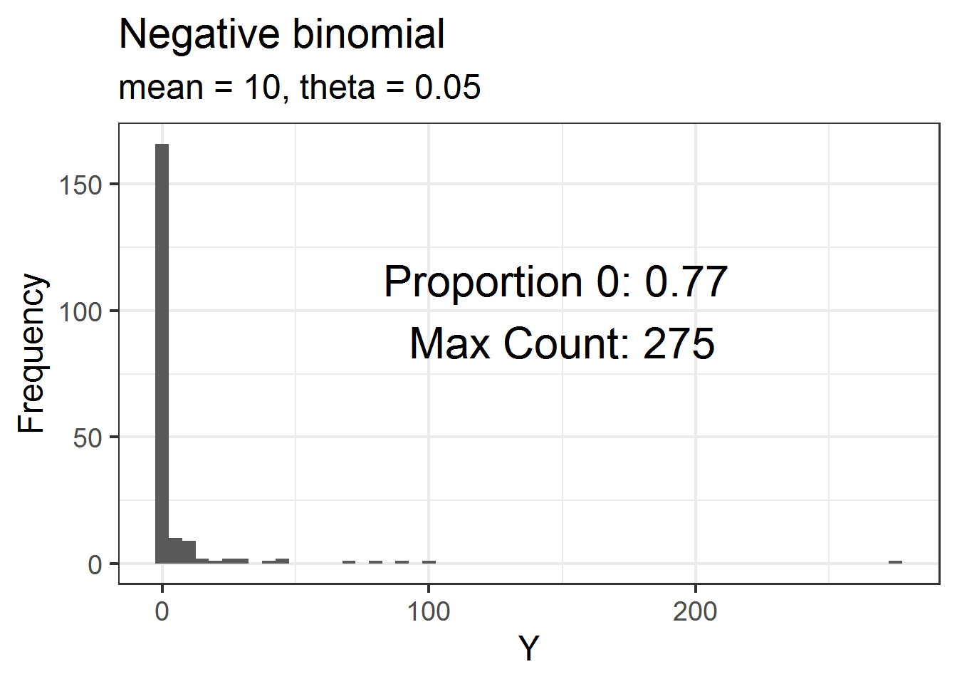
set.seed(16)
dat = data.frame(Y = rnbinom(200, mu = 10, size = .05) )
Below is a histogram of these data. I’ve annotated the plot with the proportion of the 200 values that are 0 as well as the maximum observed count in the dataset. There are lots of zeros! But these data are not zero-inflated because we expect to have many 0 values under this particular distribution.
ggplot(dat, aes(x = Y) ) +
geom_histogram(binwidth = 5) +
theme_bw(base_size = 18) +
labs(y = "Frequency",
title = "Negative binomial",
subtitle = "mean = 10, theta = 0.05" ) +
annotate(geom = "text",
label = paste("Proportion 0:", mean(dat$Y == 0),
"\nMax Count:", max(dat$Y) ),
x = 150, y = 100, size = 8)
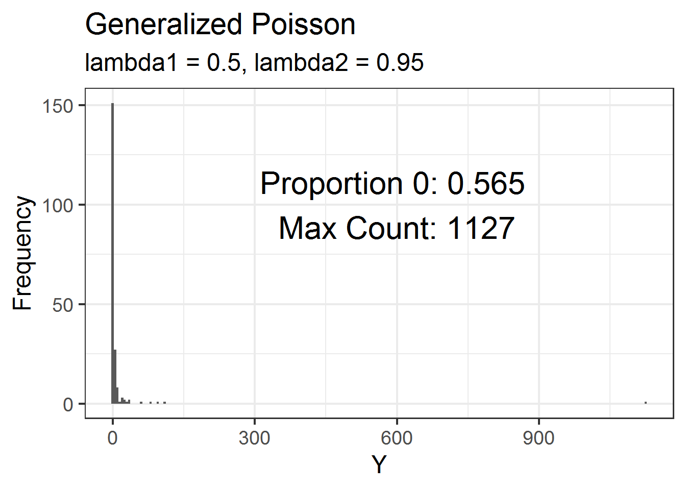
Generalized Poisson with many zeros
I don’t know the generalized Poisson distribution well, although it appears to be regularly used in some fields. For whatever reason, the negative binomial seems much more common in ecology. 🤷
From my understanding, the generalized Poisson distribution can have heavier tails than the negative binomial. This would mean that it can have more extreme maximum counts as well as lots of zeros.
See the documentation for
rgenpois()
for the formula for the density of the generalized Poisson and definitions of mean and variance. Note that when
lambda2
is 0, the generalized Poisson reduces to the Poisson.
set.seed(16)
dat = data.frame(Y = rgenpois(200, lambda1 = 0.5, lambda2 = 0.95) )
Below is a histogram of these data. Just over 50% of the values are zeros but the maximum count is over 1000! 💥
ggplot(dat, aes(x = Y) ) +
geom_histogram(binwidth = 5) +
theme_bw(base_size = 18) +
labs(y = "Frequency",
title = "Generalized Poisson",
subtitle = "lambda1 = 0.5, lambda2 = 0.95") +
annotate(geom = "text",
label = paste("Proportion 0:", mean(dat$Y == 0),
"\nMax Count:", max(dat$Y) ),
x = 600, y = 100, size = 8)
Lots of zeros or excess zeros?
All the simulations above show us is that some distributions
can
have a lot of zeros. In any given scenario, though, how do we check if we have
excess
zeros? Having excess zeros means there are more zeros than expected by the distribution we are using for modeling. If we have excess zeros than we may either need a different distribution to model the data or we could think about models that specifically address zero inflation.
The key to checking for excess zeros is to estimate the number of zeros you would expect to see if the fitted model were truly the model that created your data and compare that to the number of zeros in the actual data. If there are many more zeros in the data than the model allows for then you have zero inflation compared to whatever distribution you are using.
Simulate negative binomial data
I’ll now simulate data based on a negative binomial model with a single, continuous explanatory variable. I’ll use a model fit to these data to show how to check for excess zeros.
Since this is a generalized linear model, I first calculate the means based on the linear predictor. The exponentiation is due to using the natural log link to
link
the mean to the linear predictor.
set.seed(16)
x = runif(200, 5, 10) # simulate explanatory variable
b0 = 1 # set value of intercept
b1 = 0.25 # set value of slope
means = exp(b0 + b1*x) # calculate true means
theta = 0.25 # true theta
I can use these true means along with my chosen value of
theta
to simulate data from the negative binomial distribution.
y = rnbinom(200, mu = means, size = theta)
Now that I’ve made some data I can fit a model. Since I’m using a negative binomial GLM with
x
as the explanatory variable, which is how I created the data, this model should work well. The
glm.nb()
function is from package
MASS
.
fit1 = glm.nb(y ~ x)
In this exercise I’m going to go directly to checking for excess zeros. This means I’m skipping other important checks of model fit, such as checks for overdispersion and examining residual plots. Don’t skip these in a real analysis; having excess zeros certainly isn’t the only problem we can run into with count data.
Checking for excess zeros
The observed data has 76 zeros (out of 200).
sum(y == 0)
# [1] 76
How many zeros is expected given the model? I need the model estimated means and theta to answer this question. I can get the means via
predict()
and I can pull
theta
out of the model
summary()
.
preds = predict(fit1, type = "response") # estimated means
esttheta = summary(fit1)$theta # estimated theta
For discrete distributions like the negative binomial, the
density
distribution functions (which start with the letter “d”) return the probability that the observation is equal to a given value. This means I can use
dnbinom()
to calculate the probability of an observation being 0 for every row in the dataset. To do this I need to provide values for the parameters of the distribution of each observation.
Based on the model, the distribution of each observation is negative binomial with the mean estimated from the model and the overall estimated theta.
prop0 = dnbinom(x = 0, mu = preds, size = esttheta )
The sum of these probabilities is an estimate of the number of zero values expected by the model (see
here
for another example). I’ll round this to the nearest integer.
round( sum(prop0) )
# [1] 72
The expected number of 0 values is ~72, very close to the 76 observed in the data. This is no big surprise, since I fit the same model that I used to create the data.
An example with excess zeros
The example above demonstrates a model without excess zeros. Let me finish by fitting a model to data that has more zeros than expected by the distribution. This can be done by fitting a Poisson GLM instead of a negative binomial GLM to my simulated data.
fit2 = glm(y ~ x, family = poisson)
Remember the data contain 76 zeros.
sum(y == 0)
# [1] 76
Using
dpois()
, the number of zeros given be the Poisson model is 0. 😮 These data are zero-inflated compared to the Poisson distribution, and I clearly need a different approach for modeling these data.
round( sum( dpois(x = 0,
lambda = predict(fit2, type = "response") ) ) )
# [1] 0
This brings me back to my earlier point about checking model fit. If I had done other standard checks of model fit for
fit2
I would have seen additional problems that would indicate the Poisson distribution did not fit these data (such as severe overdispersion).
Just the code, please
Here’s the code without all the discussion. Copy and paste the code below or you can download an R script of uncommented code
from here
.
library(ggplot2) # v. 3.1.0
library(HMMpa) # v. 1.0.1
library(MASS) # v. 7.3-51.1
set.seed(16)
dat = data.frame(Y = rnbinom(200, mu = 10, size = .05) )
ggplot(dat, aes(x = Y) ) +
geom_histogram(binwidth = 5) +
theme_bw(base_size = 18) +
labs(y = "Frequency",
title = "Negative binomial",
subtitle = "mean = 10, theta = 0.05" ) +
annotate(geom = "text",
label = paste("Proportion 0:", mean(dat$Y == 0),
"\nMax Count:", max(dat$Y) ),
x = 150, y = 100, size = 8)
set.seed(16)
dat = data.frame(Y = rgenpois(200, lambda1 = 0.5, lambda2 = 0.95) )
ggplot(dat, aes(x = Y) ) +
geom_histogram(binwidth = 5) +
theme_bw(base_size = 18) +
labs(y = "Frequency",
title = "Generalized Poisson",
subtitle = "lambda1 = 0.5, lambda2 = 0.95") +
annotate(geom = "text",
label = paste("Proportion 0:", mean(dat$Y == 0),
"\nMax Count:", max(dat$Y) ),
x = 600, y = 100, size = 8)
set.seed(16)
x = runif(200, 5, 10) # simulate explanatory variable
b0 = 1 # set value of intercept
b1 = 0.25 # set value of slope
means = exp(b0 + b1*x) # calculate true means
theta = 0.25 # true theta
y = rnbinom(200, mu = means, size = theta)
fit1 = glm.nb(y ~ x)
sum(y == 0)
preds = predict(fit1, type = "response") # estimated means
esttheta = summary(fit1)$theta # estimated theta
prop0 = dnbinom(x = 0, mu = preds, size = esttheta )
round( sum(prop0) )
fit2 = glm(y ~ x, family = poisson)
sum(y == 0)
round( sum( dpois(x = 0,
lambda = predict(fit2, type = "response") ) ) ) | |||||||||||||||
| Markdown | [Very statisticious](https://aosmith.rbind.io/)
[](https://aosmith.rbind.io/#about)
#### Ariel Muldoon
##### I currently work as an applied statistician in aviation and aeronautics. In a previous role as a consulting statistician in academia I created and taught R workshops for applied science graduate students who are just getting started in R, where my goal was to make their transition to a programming language as smooth as possible. See these workshop materials at [my website](http://ariel.rbind.io/).
- [Home](https://aosmith.rbind.io/)
- [Tags](https://aosmith.rbind.io/tags)
- [About](https://aosmith.rbind.io/#about)
- [Resume](https://ariel.rbind.io/files/acm_resume.html)
- [Email](mailto:ariel.muldoon@gmail.com)
- [Twitter](https://twitter.com/aosmith16)
- [GitHub](https://github.com/aosmith16)
- [Stack Overflow](https://stackoverflow.com/users/2461552)
- [RSS](https://aosmith.rbind.io/index.xml)
- [R Weekly](https://rweekly.org/)
- [R-bloggers](https://www.r-bloggers.com/)
# Lots of zeros or too many zeros?: Thinking about zero inflation in count data
March 6, 2019
· [@aosmith16](https://twitter.com/aosmith16)\  · [View source](https://github.com/aosmith16/aosmith/blob/master/content/post/2019-03-06-lots-of-zeros.Rmd)\ 
[glmm](https://aosmith.rbind.io/tags/glmm), [simulation](https://aosmith.rbind.io/tags/simulation), [teaching](https://aosmith.rbind.io/tags/teaching)
In a recent lecture I gave a basic overview of zero-inflation in count distributions. My main take-home message to the students that I thought worth posting about here is that having a lot of zero values does not necessarily mean you have zero inflation.
Zero inflation is when there are more 0 values in the data than the distribution allows for. But some distributions can have a lot of zeros\!
## Table of Contents
- [Load packages and dataset](https://aosmith.rbind.io/2019/03/06/lots-of-zeros/#load-packages-and-dataset)
- [Negative binomial with many zeros](https://aosmith.rbind.io/2019/03/06/lots-of-zeros/#negative-binomial-with-many-zeros)
- [Generalized Poisson with many zeros](https://aosmith.rbind.io/2019/03/06/lots-of-zeros/#generalized-poisson-with-many-zeros)
- [Lots of zeros or excess zeros?](https://aosmith.rbind.io/2019/03/06/lots-of-zeros/#lots-of-zeros-or-excess-zeros)
- [Simulate negative binomial data](https://aosmith.rbind.io/2019/03/06/lots-of-zeros/#simulate-negative-binomial-data)
- [Checking for excess zeros](https://aosmith.rbind.io/2019/03/06/lots-of-zeros/#checking-for-excess-zeros)
- [An example with excess zeros](https://aosmith.rbind.io/2019/03/06/lots-of-zeros/#an-example-with-excess-zeros)
- [Just the code, please](https://aosmith.rbind.io/2019/03/06/lots-of-zeros/#just-the-code-please)
# Load packages and dataset
I’m going to be simulating counts from different distributions to demonstrate this. First I’ll load the packages I’m using today.
Package **HMMpa** is for a function to draw random samples from the generalized Poisson distribution.
```
library(ggplot2) # v. 3.1.0
library(HMMpa) # v. 1.0.1
library(MASS) # v. 7.3-51.1
```
# Negative binomial with many zeros
First I’ll draw 200 counts from a negative binomial with a mean (\\(\\lambda\\)) of \\(10\\) and \\(\\theta = 0.05\\).
R uses the parameterization of the negative binomial where the variance of the distribution is \\(\\lambda + (\\lambda^2/\\theta)\\). In this parameterization, as \\(\\theta\\) gets small the variance gets big. Using a very small value of theta like I am will generally mean the distribution of counts will have many zeros as well as a few large counts
I pull a random sample of size 200 from this distribution using `rnbinom()`. The `mu` argument is the mean and the `size` argument is theta.
```
set.seed(16)
dat = data.frame(Y = rnbinom(200, mu = 10, size = .05) )
```
Below is a histogram of these data. I’ve annotated the plot with the proportion of the 200 values that are 0 as well as the maximum observed count in the dataset. There are lots of zeros! But these data are not zero-inflated because we expect to have many 0 values under this particular distribution.
```
ggplot(dat, aes(x = Y) ) +
geom_histogram(binwidth = 5) +
theme_bw(base_size = 18) +
labs(y = "Frequency",
title = "Negative binomial",
subtitle = "mean = 10, theta = 0.05" ) +
annotate(geom = "text",
label = paste("Proportion 0:", mean(dat$Y == 0),
"\nMax Count:", max(dat$Y) ),
x = 150, y = 100, size = 8)
```
# Generalized Poisson with many zeros
I don’t know the generalized Poisson distribution well, although it appears to be regularly used in some fields. For whatever reason, the negative binomial seems much more common in ecology. 🤷
From my understanding, the generalized Poisson distribution can have heavier tails than the negative binomial. This would mean that it can have more extreme maximum counts as well as lots of zeros.
See the documentation for `rgenpois()` for the formula for the density of the generalized Poisson and definitions of mean and variance. Note that when `lambda2` is 0, the generalized Poisson reduces to the Poisson.
```
set.seed(16)
dat = data.frame(Y = rgenpois(200, lambda1 = 0.5, lambda2 = 0.95) )
```
Below is a histogram of these data. Just over 50% of the values are zeros but the maximum count is over 1000! 💥
```
ggplot(dat, aes(x = Y) ) +
geom_histogram(binwidth = 5) +
theme_bw(base_size = 18) +
labs(y = "Frequency",
title = "Generalized Poisson",
subtitle = "lambda1 = 0.5, lambda2 = 0.95") +
annotate(geom = "text",
label = paste("Proportion 0:", mean(dat$Y == 0),
"\nMax Count:", max(dat$Y) ),
x = 600, y = 100, size = 8)
```
# Lots of zeros or excess zeros?
All the simulations above show us is that some distributions *can* have a lot of zeros. In any given scenario, though, how do we check if we have *excess* zeros? Having excess zeros means there are more zeros than expected by the distribution we are using for modeling. If we have excess zeros than we may either need a different distribution to model the data or we could think about models that specifically address zero inflation.
The key to checking for excess zeros is to estimate the number of zeros you would expect to see if the fitted model were truly the model that created your data and compare that to the number of zeros in the actual data. If there are many more zeros in the data than the model allows for then you have zero inflation compared to whatever distribution you are using.
# Simulate negative binomial data
I’ll now simulate data based on a negative binomial model with a single, continuous explanatory variable. I’ll use a model fit to these data to show how to check for excess zeros.
Since this is a generalized linear model, I first calculate the means based on the linear predictor. The exponentiation is due to using the natural log link to *link* the mean to the linear predictor.
```
set.seed(16)
x = runif(200, 5, 10) # simulate explanatory variable
b0 = 1 # set value of intercept
b1 = 0.25 # set value of slope
means = exp(b0 + b1*x) # calculate true means
theta = 0.25 # true theta
```
I can use these true means along with my chosen value of `theta` to simulate data from the negative binomial distribution.
```
y = rnbinom(200, mu = means, size = theta)
```
Now that I’ve made some data I can fit a model. Since I’m using a negative binomial GLM with `x` as the explanatory variable, which is how I created the data, this model should work well. The `glm.nb()` function is from package **MASS**.
```
fit1 = glm.nb(y ~ x)
```
In this exercise I’m going to go directly to checking for excess zeros. This means I’m skipping other important checks of model fit, such as checks for overdispersion and examining residual plots. Don’t skip these in a real analysis; having excess zeros certainly isn’t the only problem we can run into with count data.
# Checking for excess zeros
The observed data has 76 zeros (out of 200).
```
sum(y == 0)
```
```
# [1] 76
```
How many zeros is expected given the model? I need the model estimated means and theta to answer this question. I can get the means via `predict()` and I can pull `theta` out of the model `summary()`.
```
preds = predict(fit1, type = "response") # estimated means
esttheta = summary(fit1)$theta # estimated theta
```
For discrete distributions like the negative binomial, the *density* distribution functions (which start with the letter “d”) return the probability that the observation is equal to a given value. This means I can use `dnbinom()` to calculate the probability of an observation being 0 for every row in the dataset. To do this I need to provide values for the parameters of the distribution of each observation.
Based on the model, the distribution of each observation is negative binomial with the mean estimated from the model and the overall estimated theta.
```
prop0 = dnbinom(x = 0, mu = preds, size = esttheta )
```
The sum of these probabilities is an estimate of the number of zero values expected by the model (see [here](https://data.library.virginia.edu/getting-started-with-hurdle-models/) for another example). I’ll round this to the nearest integer.
```
round( sum(prop0) )
```
```
# [1] 72
```
The expected number of 0 values is ~72, very close to the 76 observed in the data. This is no big surprise, since I fit the same model that I used to create the data.
# An example with excess zeros
The example above demonstrates a model without excess zeros. Let me finish by fitting a model to data that has more zeros than expected by the distribution. This can be done by fitting a Poisson GLM instead of a negative binomial GLM to my simulated data.
```
fit2 = glm(y ~ x, family = poisson)
```
Remember the data contain 76 zeros.
```
sum(y == 0)
```
```
# [1] 76
```
Using `dpois()`, the number of zeros given be the Poisson model is 0. 😮 These data are zero-inflated compared to the Poisson distribution, and I clearly need a different approach for modeling these data.
```
round( sum( dpois(x = 0,
lambda = predict(fit2, type = "response") ) ) )
```
```
# [1] 0
```
This brings me back to my earlier point about checking model fit. If I had done other standard checks of model fit for `fit2` I would have seen additional problems that would indicate the Poisson distribution did not fit these data (such as severe overdispersion).
# Just the code, please
Here’s the code without all the discussion. Copy and paste the code below or you can download an R script of uncommented code [from here](https://aosmith.rbind.io/script/2019-03-06-lots-of-zeros.R).
```
library(ggplot2) # v. 3.1.0
library(HMMpa) # v. 1.0.1
library(MASS) # v. 7.3-51.1
set.seed(16)
dat = data.frame(Y = rnbinom(200, mu = 10, size = .05) )
ggplot(dat, aes(x = Y) ) +
geom_histogram(binwidth = 5) +
theme_bw(base_size = 18) +
labs(y = "Frequency",
title = "Negative binomial",
subtitle = "mean = 10, theta = 0.05" ) +
annotate(geom = "text",
label = paste("Proportion 0:", mean(dat$Y == 0),
"\nMax Count:", max(dat$Y) ),
x = 150, y = 100, size = 8)
set.seed(16)
dat = data.frame(Y = rgenpois(200, lambda1 = 0.5, lambda2 = 0.95) )
ggplot(dat, aes(x = Y) ) +
geom_histogram(binwidth = 5) +
theme_bw(base_size = 18) +
labs(y = "Frequency",
title = "Generalized Poisson",
subtitle = "lambda1 = 0.5, lambda2 = 0.95") +
annotate(geom = "text",
label = paste("Proportion 0:", mean(dat$Y == 0),
"\nMax Count:", max(dat$Y) ),
x = 600, y = 100, size = 8)
set.seed(16)
x = runif(200, 5, 10) # simulate explanatory variable
b0 = 1 # set value of intercept
b1 = 0.25 # set value of slope
means = exp(b0 + b1*x) # calculate true means
theta = 0.25 # true theta
y = rnbinom(200, mu = means, size = theta)
fit1 = glm.nb(y ~ x)
sum(y == 0)
preds = predict(fit1, type = "response") # estimated means
esttheta = summary(fit1)$theta # estimated theta
prop0 = dnbinom(x = 0, mu = preds, size = esttheta )
round( sum(prop0) )
fit2 = glm(y ~ x, family = poisson)
sum(y == 0)
round( sum( dpois(x = 0,
lambda = predict(fit2, type = "response") ) ) )
```
[glmm](https://aosmith.rbind.io/tags/glmm/) [simulation](https://aosmith.rbind.io/tags/simulation/) [teaching](https://aosmith.rbind.io/tags/teaching/)
Please enable JavaScript to view the [comments powered by Disqus.](https://disqus.com/?ref_noscript)
© 2024 Ariel Muldoon [CC BY-SA 4.0](https://creativecommons.org/licenses/by-sa/4.0/)
- [%!(EXTRA string=Facebook)](https://www.facebook.com/sharer/sharer.php?u=https%3A%2F%2Faosmith.rbind.io%2F2019%2F03%2F06%2Flots-of-zeros%2F)
- [%!(EXTRA string=Twitter)](https://twitter.com/intent/tweet?text=https%3A%2F%2Faosmith.rbind.io%2F2019%2F03%2F06%2Flots-of-zeros%2F)

#### Ariel Muldoon
I currently work as an applied statistician in aviation and aeronautics. In a previous role as a consulting statistician in academia I created and taught R workshops for applied science graduate students who are just getting started in R, where my goal was to make their transition to a programming language as smooth as possible. See these workshop materials at [my website](http://ariel.rbind.io/). | |||||||||||||||
| Readable Markdown | In a recent lecture I gave a basic overview of zero-inflation in count distributions. My main take-home message to the students that I thought worth posting about here is that having a lot of zero values does not necessarily mean you have zero inflation.
Zero inflation is when there are more 0 values in the data than the distribution allows for. But some distributions can have a lot of zeros\!
## Table of Contents
- [Load packages and dataset](https://aosmith.rbind.io/2019/03/06/lots-of-zeros/#load-packages-and-dataset)
- [Negative binomial with many zeros](https://aosmith.rbind.io/2019/03/06/lots-of-zeros/#negative-binomial-with-many-zeros)
- [Generalized Poisson with many zeros](https://aosmith.rbind.io/2019/03/06/lots-of-zeros/#generalized-poisson-with-many-zeros)
- [Lots of zeros or excess zeros?](https://aosmith.rbind.io/2019/03/06/lots-of-zeros/#lots-of-zeros-or-excess-zeros)
- [Simulate negative binomial data](https://aosmith.rbind.io/2019/03/06/lots-of-zeros/#simulate-negative-binomial-data)
- [Checking for excess zeros](https://aosmith.rbind.io/2019/03/06/lots-of-zeros/#checking-for-excess-zeros)
- [An example with excess zeros](https://aosmith.rbind.io/2019/03/06/lots-of-zeros/#an-example-with-excess-zeros)
- [Just the code, please](https://aosmith.rbind.io/2019/03/06/lots-of-zeros/#just-the-code-please)
## Load packages and dataset
I’m going to be simulating counts from different distributions to demonstrate this. First I’ll load the packages I’m using today.
Package **HMMpa** is for a function to draw random samples from the generalized Poisson distribution.
```
library(ggplot2) # v. 3.1.0
library(HMMpa) # v. 1.0.1
library(MASS) # v. 7.3-51.1
```
## Negative binomial with many zeros
First I’ll draw 200 counts from a negative binomial with a mean (\\(\\lambda\\)) of \\(10\\) and \\(\\theta = 0.05\\).
R uses the parameterization of the negative binomial where the variance of the distribution is \\(\\lambda + (\\lambda^2/\\theta)\\). In this parameterization, as \\(\\theta\\) gets small the variance gets big. Using a very small value of theta like I am will generally mean the distribution of counts will have many zeros as well as a few large counts
I pull a random sample of size 200 from this distribution using `rnbinom()`. The `mu` argument is the mean and the `size` argument is theta.
```
set.seed(16)
dat = data.frame(Y = rnbinom(200, mu = 10, size = .05) )
```
Below is a histogram of these data. I’ve annotated the plot with the proportion of the 200 values that are 0 as well as the maximum observed count in the dataset. There are lots of zeros! But these data are not zero-inflated because we expect to have many 0 values under this particular distribution.
```
ggplot(dat, aes(x = Y) ) +
geom_histogram(binwidth = 5) +
theme_bw(base_size = 18) +
labs(y = "Frequency",
title = "Negative binomial",
subtitle = "mean = 10, theta = 0.05" ) +
annotate(geom = "text",
label = paste("Proportion 0:", mean(dat$Y == 0),
"\nMax Count:", max(dat$Y) ),
x = 150, y = 100, size = 8)
```

## Generalized Poisson with many zeros
I don’t know the generalized Poisson distribution well, although it appears to be regularly used in some fields. For whatever reason, the negative binomial seems much more common in ecology. 🤷
From my understanding, the generalized Poisson distribution can have heavier tails than the negative binomial. This would mean that it can have more extreme maximum counts as well as lots of zeros.
See the documentation for `rgenpois()` for the formula for the density of the generalized Poisson and definitions of mean and variance. Note that when `lambda2` is 0, the generalized Poisson reduces to the Poisson.
```
set.seed(16)
dat = data.frame(Y = rgenpois(200, lambda1 = 0.5, lambda2 = 0.95) )
```
Below is a histogram of these data. Just over 50% of the values are zeros but the maximum count is over 1000! 💥
```
ggplot(dat, aes(x = Y) ) +
geom_histogram(binwidth = 5) +
theme_bw(base_size = 18) +
labs(y = "Frequency",
title = "Generalized Poisson",
subtitle = "lambda1 = 0.5, lambda2 = 0.95") +
annotate(geom = "text",
label = paste("Proportion 0:", mean(dat$Y == 0),
"\nMax Count:", max(dat$Y) ),
x = 600, y = 100, size = 8)
```

## Lots of zeros or excess zeros?
All the simulations above show us is that some distributions *can* have a lot of zeros. In any given scenario, though, how do we check if we have *excess* zeros? Having excess zeros means there are more zeros than expected by the distribution we are using for modeling. If we have excess zeros than we may either need a different distribution to model the data or we could think about models that specifically address zero inflation.
The key to checking for excess zeros is to estimate the number of zeros you would expect to see if the fitted model were truly the model that created your data and compare that to the number of zeros in the actual data. If there are many more zeros in the data than the model allows for then you have zero inflation compared to whatever distribution you are using.
## Simulate negative binomial data
I’ll now simulate data based on a negative binomial model with a single, continuous explanatory variable. I’ll use a model fit to these data to show how to check for excess zeros.
Since this is a generalized linear model, I first calculate the means based on the linear predictor. The exponentiation is due to using the natural log link to *link* the mean to the linear predictor.
```
set.seed(16)
x = runif(200, 5, 10) # simulate explanatory variable
b0 = 1 # set value of intercept
b1 = 0.25 # set value of slope
means = exp(b0 + b1*x) # calculate true means
theta = 0.25 # true theta
```
I can use these true means along with my chosen value of `theta` to simulate data from the negative binomial distribution.
```
y = rnbinom(200, mu = means, size = theta)
```
Now that I’ve made some data I can fit a model. Since I’m using a negative binomial GLM with `x` as the explanatory variable, which is how I created the data, this model should work well. The `glm.nb()` function is from package **MASS**.
```
fit1 = glm.nb(y ~ x)
```
In this exercise I’m going to go directly to checking for excess zeros. This means I’m skipping other important checks of model fit, such as checks for overdispersion and examining residual plots. Don’t skip these in a real analysis; having excess zeros certainly isn’t the only problem we can run into with count data.
## Checking for excess zeros
The observed data has 76 zeros (out of 200).
```
sum(y == 0)
```
```
# [1] 76
```
How many zeros is expected given the model? I need the model estimated means and theta to answer this question. I can get the means via `predict()` and I can pull `theta` out of the model `summary()`.
```
preds = predict(fit1, type = "response") # estimated means
esttheta = summary(fit1)$theta # estimated theta
```
For discrete distributions like the negative binomial, the *density* distribution functions (which start with the letter “d”) return the probability that the observation is equal to a given value. This means I can use `dnbinom()` to calculate the probability of an observation being 0 for every row in the dataset. To do this I need to provide values for the parameters of the distribution of each observation.
Based on the model, the distribution of each observation is negative binomial with the mean estimated from the model and the overall estimated theta.
```
prop0 = dnbinom(x = 0, mu = preds, size = esttheta )
```
The sum of these probabilities is an estimate of the number of zero values expected by the model (see [here](https://data.library.virginia.edu/getting-started-with-hurdle-models/) for another example). I’ll round this to the nearest integer.
```
round( sum(prop0) )
```
```
# [1] 72
```
The expected number of 0 values is ~72, very close to the 76 observed in the data. This is no big surprise, since I fit the same model that I used to create the data.
## An example with excess zeros
The example above demonstrates a model without excess zeros. Let me finish by fitting a model to data that has more zeros than expected by the distribution. This can be done by fitting a Poisson GLM instead of a negative binomial GLM to my simulated data.
```
fit2 = glm(y ~ x, family = poisson)
```
Remember the data contain 76 zeros.
```
sum(y == 0)
```
```
# [1] 76
```
Using `dpois()`, the number of zeros given be the Poisson model is 0. 😮 These data are zero-inflated compared to the Poisson distribution, and I clearly need a different approach for modeling these data.
```
round( sum( dpois(x = 0,
lambda = predict(fit2, type = "response") ) ) )
```
```
# [1] 0
```
This brings me back to my earlier point about checking model fit. If I had done other standard checks of model fit for `fit2` I would have seen additional problems that would indicate the Poisson distribution did not fit these data (such as severe overdispersion).
## Just the code, please
Here’s the code without all the discussion. Copy and paste the code below or you can download an R script of uncommented code [from here](https://aosmith.rbind.io/script/2019-03-06-lots-of-zeros.R).
```
library(ggplot2) # v. 3.1.0
library(HMMpa) # v. 1.0.1
library(MASS) # v. 7.3-51.1
set.seed(16)
dat = data.frame(Y = rnbinom(200, mu = 10, size = .05) )
ggplot(dat, aes(x = Y) ) +
geom_histogram(binwidth = 5) +
theme_bw(base_size = 18) +
labs(y = "Frequency",
title = "Negative binomial",
subtitle = "mean = 10, theta = 0.05" ) +
annotate(geom = "text",
label = paste("Proportion 0:", mean(dat$Y == 0),
"\nMax Count:", max(dat$Y) ),
x = 150, y = 100, size = 8)
set.seed(16)
dat = data.frame(Y = rgenpois(200, lambda1 = 0.5, lambda2 = 0.95) )
ggplot(dat, aes(x = Y) ) +
geom_histogram(binwidth = 5) +
theme_bw(base_size = 18) +
labs(y = "Frequency",
title = "Generalized Poisson",
subtitle = "lambda1 = 0.5, lambda2 = 0.95") +
annotate(geom = "text",
label = paste("Proportion 0:", mean(dat$Y == 0),
"\nMax Count:", max(dat$Y) ),
x = 600, y = 100, size = 8)
set.seed(16)
x = runif(200, 5, 10) # simulate explanatory variable
b0 = 1 # set value of intercept
b1 = 0.25 # set value of slope
means = exp(b0 + b1*x) # calculate true means
theta = 0.25 # true theta
y = rnbinom(200, mu = means, size = theta)
fit1 = glm.nb(y ~ x)
sum(y == 0)
preds = predict(fit1, type = "response") # estimated means
esttheta = summary(fit1)$theta # estimated theta
prop0 = dnbinom(x = 0, mu = preds, size = esttheta )
round( sum(prop0) )
fit2 = glm(y ~ x, family = poisson)
sum(y == 0)
round( sum( dpois(x = 0,
lambda = predict(fit2, type = "response") ) ) )
``` | |||||||||||||||
| ML Classification | ||||||||||||||||
| ML Categories |
Raw JSON{
"/Science": 736,
"/Science/Mathematics": 690,
"/Science/Mathematics/Statistics": 678,
"/Computers_and_Electronics": 137,
"/Computers_and_Electronics/Software": 100
} | |||||||||||||||
| ML Page Types |
Raw JSON{
"/Article": 996,
"/Article/Tutorial_or_Guide": 958
} | |||||||||||||||
| ML Intent Types |
Raw JSON{
"Informational": 999
} | |||||||||||||||
| Content Metadata | ||||||||||||||||
| Language | null | |||||||||||||||
| Author | Ariel Muldoon | |||||||||||||||
| Publish Time | 2019-03-06 00:00:00 (7 years ago) | |||||||||||||||
| Original Publish Time | 2019-03-06 00:00:00 (7 years ago) | |||||||||||||||
| Republished | No | |||||||||||||||
| Word Count (Total) | 1,894 | |||||||||||||||
| Word Count (Content) | 1,682 | |||||||||||||||
| Links | ||||||||||||||||
| External Links | 11 | |||||||||||||||
| Internal Links | 16 | |||||||||||||||
| Technical SEO | ||||||||||||||||
| Meta Nofollow | No | |||||||||||||||
| Meta Noarchive | No | |||||||||||||||
| JS Rendered | No | |||||||||||||||
| Redirect Target | null | |||||||||||||||
| Performance | ||||||||||||||||
| Download Time (ms) | 844 | |||||||||||||||
| TTFB (ms) | 843 | |||||||||||||||
| Download Size (bytes) | 7,412 | |||||||||||||||
| Shard | 166 (laksa) | |||||||||||||||
| Root Hash | 13779606198685285766 | |||||||||||||||
| Unparsed URL | io,rbind!aosmith,/2019/03/06/lots-of-zeros/ s443 | |||||||||||||||